Weak Lensing Mass Measurements of Substructures in COMA Cluster with Subaru/Suprime-Cam

Abstract

We obtain the projected mass distributions for two Subaru/Suprime-Cam fields in the southwest region ($r\lower 2.15277pt\hbox{$\;\buildrel<\over{\sim}\;$}60\farcm$) of the Coma cluster ($z=0.0236$) by weak lensing analysis and detect eight subclump candidates. We quantify the contribution of background large-scale structure (LSS) on the projected mass distributions using SDSS multi-bands and photometric data, under the assumption of mass-to-light ratio for field galaxies. We find that one of eight subclump candidates, which is not associated with any member galaxies, is significantly affected by LSS lensing. The mean projected mass for seven subclumps extracted from the main cluster potential is $\langle M_{{\rm 2D}}^{\rm(corr)}\rangle=(5.06\pm 1.30)\times 10^{12}h^{-1}M_{\sun}$ after a LSS correction. A tangential distortion profile over an ensemble of subclumps is well described by a truncated singular-isothermal sphere model and a truncated NFW model. A typical truncated radius of subclumps, $r_{t}\simeq 35~{}h^{-1}{\rm kpc}$, is derived without assuming any relations between mass and light for member galaxies. The radius coincides well with the tidal radius, $\sim 42~{}h^{-1}{\rm kpc}$, of the gravitational force of the main cluster. Taking into account the incompleteness of data area, a projection effect and spurious lensing peaks, it is expected that mass of cluster substructures account for $19$ percent of the virial mass, with $13$ percent statistical error. The mass fraction of cluster substructures is in rough agreement with numerical simulations.

1. Introduction

The cold dark matter (CDM) paradigm predicts the presence of numerous substructures in dark halos on any scale, because less massive objects form earlier and become more massive through mergers. Indeed, high-resolution N-body simulations have shown an assemble history that subhalos continually fall into larger halos. When interior subhalos penetrate into a central region of a massive parent halo, subhalos are disrupted by its strong tidal field. As a result, the original subhalo mass is reduced by the tidal effect and becomes a part of smoothed component of the parent halo (e.g De Lucia et al. 2004; Gao et al. 2004). Therefore, a study of subhalo properties is of vital importance to understand an assemble history in halo environments. Furthermore, a statistical study for subhalos, such as mass function, would offer a powerful test of the CDM model on scales less than several Mpc.

Gravitational lensing analysis on background galaxies is the unique technique to map out mass distributions of any object, such as galaxies and clusters, regardless of the dynamical state. It therefore enables us to explore substructures in primary halos and to measure directly their masses. Indeed, galaxy-galaxy lensing studies in clusters (e.g. Natarajan & Springel 2004; Natarajan, De Lucia & Springel 2007) revealed cluster substructures and measured their mass functions under the assumption of a scaling relation between mass and light. However, a technique requiring no assumption of mass-to-light relation is of paramount importance, because subhalo size in a strong tidal field depends on its orbit parameters as well. Furthermore, we cannot rule out a possibility that gaseous galaxies in a gaseous environment of galaxy clusters are offset from subhalo centers because of ram pressure. Even a slight offset prevents us from measuring subhalo masses accurately, because a mis-centering of tangential distortion profile causes large error in mass estimations especially within inner regions (e.g Yang et al 2006; Johnston et al. 2007). It is therefore of importance to explore subhalos and measure their masses based on a weak mass reconstruction technique independent of any mass-to-light scaling relations.

As demonstrated by Okabe & Umetsu (2008), a systematic weak lensing study on seven mering clusters in the range of $z\sim 0.055-0.28$ is capable of discovering massive substructures associated with cluster major majors. However, the limit of angular resolution of reconstructed mass distributions, within the redshift range, makes it difficult to discover less massive substructures associated with cluster galaxies. On the other hand, it would be easier to detect less massive substructures in lower redshift clusters in spite of the weakness of their lensing signal, because the number of available source galaxies increases thanks to larger apparent size of objects at lower redshift. Therefore, weak lensing study of low-redshift clusters will provides us with a good opportunity to detect and measure smaller subhalo masses in clusters. As the first step, we select Coma cluster for the target to measure subhalo masses by weak lensing analysis alone. The redshift of Coma cluster is 0.0236 and is known as one of the most massive clusters near us. We analyze archival Subaru/Suprime-Cam data (Miyazaki et al. 2002) to measure subhalo masses found in projected mass distributions as well as cluster virial mass, and calculate the mass fraction of substructures. We also investigate lensing from background large-scale structure (LSS) in a quantitative way, using SDSS multi-bands and photometric data.

The outline of this paper is as follows. We briefly describe the data analysis in §2 and measure the three-dimensional mass enclosed within a spherical region of a given radius using a tangential shear profile in §3. §4 represents projected distributions of mass and member galaxies, quantifies false lensing peaks and estimate background lensing effects on the weak lensing mass reconstruction. In §5, we measure the two-dimensional masses for subclumps with and without LSS lensing correction. In §6, we fit a tangential shear profile over an ensemble of subclump candidates and obtain the typical truncated radius and mass of subhalos. §7 is devoted to the discussion. Throughout the paper we adopt cosmology parameters $\Omega_{m0}=0.27$ and $\Omega_{\Lambda}=0.73$. At the redshift of Coma cluster $1\farcm=20.0h^{-1}{\rm kpc}$.

2. Data Analysis

We retrieved two $R_{\rm c}$ image data (Yoshida et al. 2008) from the Subaru archival data (SMOKA). Pointings of imaging data are the central region of $r\lower 2.15277pt\hbox{$\;\buildrel<\over{\sim}\;$}30\farcm$ from cD galaxy NGC4874 and the outskirts region of $r\sim 30-60\farcm$. They cover the southwest part of this cluster. The data were reduced by the same imaging process of using standard pipeline reduction software for Suprime-Cam, SDFRED (Yagi et al., 2002; Ouchi et al., 2004), as described in Okabe & Umetsu (2008). Astrometry and the photometric calibration were conducted using the Sloan Digital Sky Survey (SDSS) data catalog. The exposure times are $42$ and $16$ minutes for the central and outskirt regions, respectively.

Our weak lensing analysis was done using the IMCAT package provided by N. Kaiser(Kaiser, Squires & Broadhurst 1995). We use the same pipeline as Okabe et al. (2009) with some modifications followed by Erben et al. (2001) (also see Okabe & Umetsu 2008). In the pipeline, we first measure the image ellipticity, $e_{\alpha}$, from the weighted quadrupole moments of the surface brightness of each object and then correct the PSF anisotropy as $e_{\alpha}^{\prime}=e_{\alpha}-P_{\rm sm}^{\alpha\beta}(P_{\rm sm}*)^{-1}_{\beta\gamma}e^{\gamma}*$, where $P_{\alpha\beta}$ is the smear polarizablity tensor and the asterisk denotes the stellar objects. We fit the stellar anisotropy kernel $(P_{\rm sm}*)^{-1}_{\alpha\beta}e^{\beta}*$ with the second-order bi-polynomials function in several subimages whose sizes are determined based on the typical coherent scale of the measured PSF anisotropy pattern. We finally obtain the reduced shear $g_{\alpha}=\gamma_{\alpha}/(1-\kappa)=(P_{g})_{\alpha\beta}^{-1}e_{\beta}^{\prime}$ using the pre-seeing shear polarizablity tensor $P_{g}$. We adopt the scalar value $(P_{g})_{\alpha\beta}={\rm Tr}[P_{g}]\delta_{\alpha\beta}/2$, following the technique described in Erben (2001).

We ran the pipeline for each imaging data and obtained the shear catalogue of source galaxies whose magnitude ranges are $20-25$ ABmag and half-light-radius are $\bar{r}_{h}^{*}+\sigma(r_{h}^{*})<r_{h}<10$ pixel, where $\bar{r}_{h}^{*}$ and $\sigma(r_{h}^{*})$ are the mean and $1\sigma$ error for stellar objects, respectively. Here the upper limit of magnitude is determined by the outskirt data of short exposure time, although faint galaxies in the range of $25-26$AB mag are usable in the data of central region. Since apparent sizes of unlensed galaxies, mainly cluster members, are large in general, our source galaxy selection efficiently excludes member galaxies which dilutes lensing strengths. The number density of source galaxies is $\simeq 23{\rm~{}arcmin}^{-2}$.

3. Cluster Mass Measurement

We measure a tangential shear component, $g_{+}=-g_{1}\cos 2\varphi-g_{2}\sin 2\varphi$ and the $45$ degree rotated component, $g_{\times}=-g_{1}\sin 2\varphi+g_{2}\cos 2\varphi$, with respect to the cluster center, where $\varphi$ is the position angle in counter clockwise direction from the first coordinate. Then, the profiles of shear components $g_{\beta}=(g_{+},g_{\times})$ are obtained from the weighted azimuthal average of the distortion components of source galaxies as $\langle{g_{\beta}}\rangle(\theta_{n})=\sum_{i}u_{g,i}g_{\beta,i}/\sum_{i}u_{g,i}$ with a statistical weight $u_{g,i}=1/(\sigma_{g,i}^{2}+\alpha^{2})$, where subscripts ’n’ and ’i’ denote the n-th radial bin and i-th source object. We adopt the softening constant $\alpha=0.4$ which is a typical value of the mean rms ${\bar{\sigma}}_{g}$ over source galaxies.

There are two cD galaxies (NGC 4874 and NGC 4889) in the central region of Coma cluster. We adopt the center of Coma cluster as NGC 4874 because a number of luminous galaxies are concentrated around NGC 4874 in our optical image, and the peak of X-ray surface brightness is close to NGC 4874 (see also Figure 10). The shear profile covers the range of $4\farcm-60\farcm$ with 5 bins. It corresponds to the first bin of Kubo et al. (2007). We fit the shear profile with the universal profile proposed by Navarro, Frenk & White (1996; hereafter NFW profile) and a singular isothermal sphere (SIS) halo model. We assume that the redshift of source background galaxies is $\langle z_{s}\rangle=1$. An uncertainty of source redshift in mass estimates is negligible because the lens distance ratio, $D_{ls}/D_{s}$, at such a low redshift cluster weakly depends on source redshifts.

The NFW mass model is described by two parameters of the three-dimensional mass $M_{\rm NFW}(<r_{\Delta})$ and the halo concentration $c_{\rm\Delta}=r_{\Delta}/r_{s}$, where $r_{s}$ is a scale radius and $r_{\Delta}$ is a radius at which the mean density is $\Delta$ times the critical mass density, $\rho_{\rm cr}(z)$, at the cluster redshift. The density profile of NFW mass model is expressed in the form of

$$\rho_{\rm NFW}(r)=\frac{\rho_{s}}{(r/r_{s})(1+r/r_{s})^{2}}.$$ (1)

The three-dimensional cluster mass for NFW mass model is obtained by

$$M_{\rm NFW}(<r_{\Delta})=\frac{4\pi\rho_{s}r_{\Delta}^{3}}{c_{\Delta}^{3}}m(c_{\Delta}),$$ (2)

with

$$m(x) = \log(1+x)-\frac{x}{1+x}.$$ (3)

For reference with other works, results of mass and concentration parameter within radii for $\Delta=2500,500$ & $200$ and virial overdensity $\Delta=\Delta_{\rm vir}\simeq 98$ (Nakamura & Suto 1997), are listed in Table 1. The density profile for SIS mass model is given by

$$\rho_{\rm SIS}(r) = \frac{\sigma_{v}^{2}}{2\pi Gr^{2}},$$ (4)

where the one-dimensional velocity dispersion, $\sigma^{2}_{v}$, is a parameter.

The resulting parameters are summarized in Table 1. Since the covering area of the data is small $\lower 2.15277pt\hbox{$\;\buildrel<\over{\sim}\;$}60\farcm$, the NFW mass is not constrained well. This is why the mass $M_{\Delta}$ determined by fitting the tangential shear is sensitive to the tangential distortion at $r_{\Delta}$ (Okabe et al. 2009). Since the best-fit virial radius is $\sim 98\farcm 5$, we require data of wider region to measure the cluster mass accurately. We note that the $\chi^{2}$ is quite small because the number of background galaxies is scarce and the intrinsic ellipticity noise is large. The covering area of our data is only $\sim 16\%$ within $60\farcm$. If the data covers whole area, the error would improve $\sim 2.5$ times and the $\chi^{2}$ would become close to $1$. The NFW virial mass changes $-0.5\%$ and $+0.8\%$ if the mean source redshift is changed to $\langle z_{s}\rangle=1.2$ and $0.8$, respectively.

We also perform a fitting taking into account a large-scale structure (LSS) lensing effect. The estimation of LSS effect on lensing signal will be described in detail in §4.4. The best-fit parameters are summarized in Table 2. The LSS effect is not significant on cluster mass estimate.

Figure 1.— Profiles of tangential shear component (top panel), $g_{+}$, and the $45$ degree rotated component (bottom panel), $g_{\times}$. The solid and dashed lines are the best-fit NFW and SIS models, respectively

.

Table 1Best-fit Mass Models without a LSS lensing correction

NFW	$\chi^{2}/{\rm d.o.f}=0.1/3$
$\Delta$	$M_{\rm NFW}(<r_{\Delta})$	$c_{\Delta}$	$r_{\Delta}$	$\theta_{\Delta}$
	$10^{14}h^{-1}M_{\sun}$		$h^{-1}$kpc	arcmin
(1)	(2)	(3)	(4)	(5)
vir	$8.85_{-5.12}^{+19.87}$	$3.49_{-1.78}^{+2.55}$	$1972.2_{-493.7}^{+947.7}$	$98.30_{-24.54}^{+47.19}$
$200$	$6.56_{-3.60}^{+11.93}$	$2.49_{-1.34}^{+1.93}$	$1403.7_{-326.8}^{+579.2}$	$70.15_{-16.33}^{+28.94}$
$500$	$4.05_{-2.00}^{+5.01}$	$1.53_{-0.90}^{+1.34}$	$880.7_{-177.6}^{+270.5}$	$44.01_{-8.87}^{+13.52}$
$2500$	$1.18_{-0.42}^{+0.57}$	$0.61_{-0.40}^{+0.67}$	$341.2_{-46.3}^{+47.5}$	$17.05_{-2.31}^{+2.38}$
SIS	$\chi^{2}/{\rm d.o.f}=4.4/4$
$\sigma_{v}$ (km/s)
(6)
$671.1_{-69.5}^{+73.4}$

Table 2Best-Fit Mass Models with a LSS lensing correction (see §3 & §4.4)

NFW	$\chi^{2}/{\rm d.o.f}=0.1/3$
$\Delta$	$M_{\rm NFW}(<r_{\Delta})$	$c_{\Delta}$	$r_{\Delta}$	$\theta_{\Delta}$
	$10^{14}h^{-1}M_{\sun}$		$h^{-1}$kpc	arcmin
(1)	(2)	(3)	(4)	(5)
vir	$8.92_{-5.17}^{+20.05}$	$3.50_{-1.79}^{+2.56}$	$1972.2_{-493.7}^{+947.7}$	$98.56_{-24.67}^{+47.36}$
$200$	$6.61_{-3.63}^{+12.06}$	$2.50_{-1.34}^{+1.94}$	$1407.7_{-328.4}^{+581.6}$	$70.35_{-16.41}^{+29.07}$
$500$	$4.09_{-2.01}^{+5.07}$	$1.57_{-0.90}^{+1.34}$	$883.4_{-178.0}^{+272.0}$	$44.15_{-8.90}^{+13.59}$
$2500$	$1.19_{-0.42}^{+0.58}$	$0.61_{-0.40}^{+0.67}$	$342.5_{-45.0}^{+47.7}$	$17.11_{-2.25}^{+2.38}$
SIS	$\chi^{2}/{\rm d.o.f}=4.4/4$
$\sigma_{v}$ (km/s)
(6)
$673.0_{-69.7}^{+73.7}$

4. Projected Distributions of Mass and Galaxies

4.1. Mass, Number Density and Luminosity Maps

We reconstruct the lensing convergence field, $\kappa$, from the shear field, using the Kaiser & Squires inversion method (Kaiser & Squires 1993), following Okabe & Umetsu (2008). In the map making, we pixelize the shear data into a pixel grid using a Gaussian smoothing kernel $w_{g}(\theta)\propto\exp[-\theta^{2}/\theta_{g}^{2}]$ and a statistical weight $u_{g,i}$ (§3). The shear field at a given position ($\theta$) is obtained by $\bar{\gamma}_{\alpha}(\mbox{\boldmath$\theta$})=\sum_{i}w_{g}(\mbox{\boldmath$\theta$}-\mbox{\boldmath$\theta$}_{i})u_{g,i}\gamma_{\alpha,i}/\sum_{i}w_{g}(\mbox{\boldmath$\theta$}-\mbox{\boldmath$\theta$}_{i})u_{g,i}$, where the weak limit $g_{\alpha}\approx\gamma_{\alpha}$ is assumed. We employ the smoothing ${\rm FWHM}=\sqrt{4\ln{2}}\theta_{g}=2\farcm 00$. The error variance for the smoothed shear is given as $\sigma^{2}_{\bar{g}}(\mbox{\boldmath$\theta$})=(\sum_{i}w_{g}(\mbox{\boldmath$\theta$}-\mbox{\boldmath$\theta$}_{i})^{2}u_{g,i}^{2}\sigma^{2}_{g,i})/\left(\sum_{i}w_{g}(\mbox{\boldmath$\theta$}-\mbox{\boldmath$\theta$}_{i})u_{g,i}\right)^{2}$. We have used $\langle g_{\alpha,i}\,g_{\beta,j}\rangle=(1/2)\sigma_{g,i}^{2}\delta^{\rm K}_{\alpha\beta}\delta^{\rm K}_{ij}$ with $\delta^{\rm K}_{\alpha\beta}$ and $\delta_{ij}^{\rm K}$ being the Kronecker’s delta. In the linear map-making process, the pixelized shear field is weighted by the inverse of the variance.

The resulting E-mode and B-mode map of lensing fields are shown in panels B and C in Figures 2 and 3 which cover the central region ($26\farcm\times 26\farcm$) and the outskirts ($21\farcm\times 21\farcm$), respectively. Contours are spaced in a unit of $1\sigma$ reconstructed errors. As seen in panels A and B, we find eight candidates of mass clumps whose significance is over $3\sigma$ level. The panel A in Figures 2 and 3 show the Subaru $R_{\rm c}$-band images overlaid with contours of reconstructed mass distributions. We labeled subclumps as shown in panel A. The significance levels of mass clumps are lower than those of other clusters at redshift range $z\sim 0.055-0.28$ (Okabe & Umetsu 2008). The B-mode map (panel C) in the central region shows 2 clumps over $3\sigma$ close to clump candidates 4 and 2 ($3.5\sigma$ and $3.9\sigma$).

We retrieve the SDSS DR7 catalogue (Abazajian et al. 2009) from SDSS CasJobs site in order to investigate member galaxy distributions. We select bright member galaxies by criteria of $i^{\prime}<19$ ABmag and $|(g^{\prime}-i^{\prime})-(-0.05i^{\prime}+2.04)|<0.14$, where we use psfMag for magnitude and modelcolor for color. We convert from apparent to absolute magnitudes by using the k-correction for early-type galaxies under the assumption that all member galaxies are located at a single cluster redshift. The galaxy luminosity and density projected distributions are obtained using the same kernel of weak lensing mass reconstruction. The overall mass distribution appears to be similar to the galaxy luminosity and density distributions. In particular, the 6 out of 8 mass candidates, but for the clumps 3 and 5, host bright galaxies. At the clump candidate 3, groups of faint member galaxies were known (Conselice & Gallagher 1999), while any galaxy group are not found at the candidate 5 region. We list the luminous galaxy associated with each candidate in Table 3. We do not always detect mass structures for all known groups or luminous galaxies. There are three possibilities for this. First, the large-scale-structure (LSS) lensing effect prevents us from detecting lensing signals. Second, dark matter halos associated with almost member galaxies are less massive than the detection limit ($3\sigma$), $3\times(\pi\theta_{g}^{2}\Sigma_{\rm cr}\delta\kappa)\sim 3\times 10^{12}h^{-1}M_{\sun}$. Third, dark halos lost their mass by the tidal force of the main cluster and then are smoothly distributed within the smoothing scale of mass reconstruction.

4.2. Bootstrap Re-sampling Mass Reconstructions

We run 1000 bootstrap simulations for making mass reconstruction in order to investigate the realization of mass clumps. In each reconstruction, we generate a bootstrap data-set by choosing randomly galaxies, with replacement, from the original shear catalogue and then identify mass clumps whose significance level is more than $3\sigma$. Figure 4 shows the resulting distributions of histogram of the appearance of mass peaks These distributions are well associated with mass clumps. The radii at which $68\%$ of the centroid positions contain are $0\farcm 8-3\farcm$. Therefore, the detected lensing peaks are realized well in the shear catalogue.

4.3. Monte-Carlo Realizations

We next construct a noise map, $\kappa_{\rm rms}$, from $1000$ Monte-Carlo realizations, following Miyazaki et al. (2007). The position and shear components of background galaxy catalogue are randomly shuffled in each realization. A mass map for a new background catalogue is reconstructed by applying the same procedure as making the original $\kappa$ maps. We estimate the rms noise in each pixel and make the noise maps, $\kappa_{\rm rms}$ for the central region and the outskirts. Noise maps are not changed even if we randomly choose half of catalogue. The significance maps, $\nu=\kappa/\kappa_{\rm rms}$, are obtained by dividing the original $\kappa$ maps by the $\kappa_{\rm rms}$ map. The resulting $\nu$ and $\kappa_{\rm rms}$ maps for both E- and B-modes are shown in Figure 5. The variation along the left and top edges of $\kappa_{\rm rms}$ map in the central region is smaller than the other region. This is why fewer galaxies exist around the boundary of the optical image. The significance maps, $\nu$, are consistent with the original E- and B-mode maps. The significance for subclump candidates, $\nu$, is also consistent with the original $S/N$ ratio (Table 3).

Are positions of E-mode and B-mode peaks correlated ? In the central region, two B-mode peaks whose significance level is above $3\sigma$ are appeared close to E-mode peaks. We calculate the probability, $P_{\rm EB}$, as function of the distance between E- and B-mode peaks appeared in Monte-Carlo realizations. The following result does not change even when we use half of realization data. Since the appearance probability is proportional to the area size, we also compute the probability, $P_{\rm rnd}$, that E- and B-mode peaks are randomly and independently located in each pixel. Figure 6 shows the appearance probabilities, $P_{\rm EB}$, for the central region and the outskirts, which roughly agrees with the probability of white noise case. A slight excess of the ratio $P_{\rm EB}/P_{\rm rnd}$ is found in the range of $\theta<10\farcm$, but the probability is quite small. Since they are not significant, we cannot identify fake E-mode peaks using the distance from B-mode peaks. The probabilities of large distance $>20\farcm$ is smaller than the unity, because few peaks are appeared around the edge. Indeed, the appearance probability in one pixel within $2\farcm$ width from the boundary is about one-thirds of that in the rest region. The probability of spurious lensing peaks will be evaluated considering the large-scale structure lensing effect §4.5.

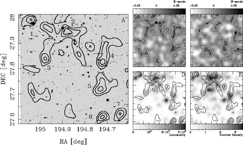
Figure 2.— The panel A is Subaru $R_{\rm c}$-band image of the central $26\farcm\times 26\farcm$ cluster region. Two cD galaxies (NGC 4874 and NGC 4889) are located around the northeast boundary. Overlaid are contours of the reconstructed projected mass distribution, spaced in a unit of $1\sigma$ reconstruction error ($\delta\kappa=0.018$). The Gaussian FWHM is $2\farcm 00$. The identified subclumps are labeled in the panel A. The panels B and C are the lensing $\kappa$ (E-mode) and B-mode fields. The panels D and E are cluster luminosity and density distributions in SDSS $i^{\prime}$-band smoothed to the same angular resolution of the mass map, respectively. Seven clump candidates are found in the central region.

.

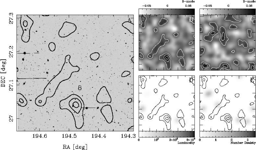
Figure 3.— The panel A is Subaru $R_{\rm c}$-band image of the outskirts $21\farcm\times 21\farcm$ cluster region. Overlaid are contours of the reconstructed projected mass distribution, spaced in a unit of $1\sigma$ reconstruction error ($\delta\kappa=0.020$). The Gaussian FWHM is $2\farcm 00$. The identified subclumps are labeled in the panel A. The panels B and C are the lensing $\kappa$ (E-mode) and B-mode fields. The clump 8 is far $\sim 58\farcm$ from cD galaxy NGC4874. The panels D and E are cluster luminosity and density distributions in SDSS $i^{\prime}$-band smoothed to the same angular resolution of the mass map, respectively. One clump candidate is found in the outskirts.

.

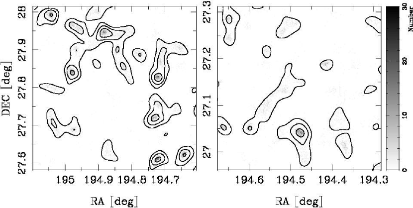
Figure 4.— The histogram maps of centroid of mass peaks, whose significance level is above $3\sigma$, appeared in 1000 bootstrap re-sampling mass-reconstructions. Contours are the same as Figures 2 and 3. Left and right panels are the central and outskirts regions, respectively.

             

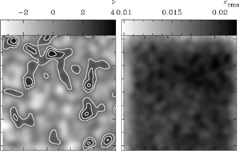
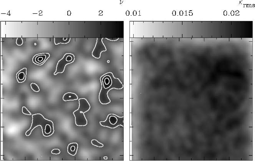
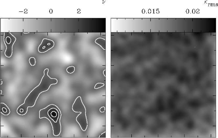
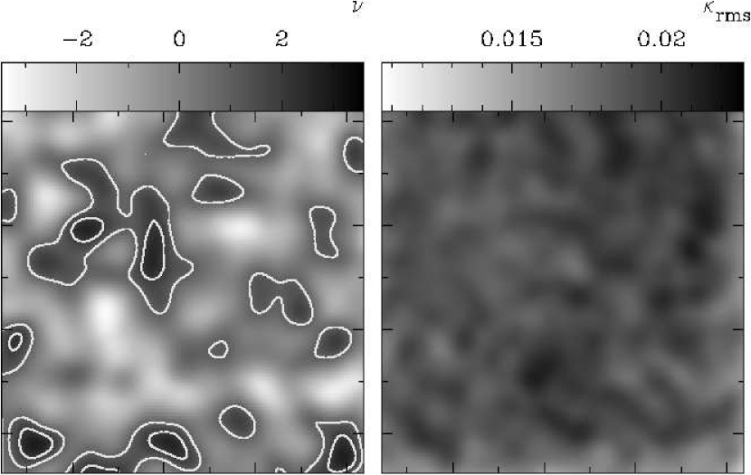
Figure 5.— Top-left: The maps for significance $\nu=\kappa/\kappa_{\rm rms}$ (left) and noise $\kappa_{\rm rms}$ (right) for E-mode in the central region, based on 1000 Monte-Carlo realizations. The contours are spaced by $\nu=1,2,$ and $3$. Top-right: The same maps for B-mode in the central region as the top-left panel. Bottom-left: The same maps for E-mode in the outskirts. Bottom-right: The same maps for B-mode in the outskirts.

Figure 6.— Top: The appearance probabilities as a function of distance between E- and B-mode peaks for the central region and the outskirts. $P_{\rm EB}$ is the appearance probability obtained by 1000 Monte-Carlo realizations. $P_{\rm rnd}$ is the probability that E- and B-mode peaks are randomly and independently appeared. Middle: The ratio of $P_{\rm EB}/P_{\rm rnd}$ for the central region. Bottom: The ratio of $P_{\rm EB}/P_{\rm rnd}$ for the outskirts.

4.4. Projection Effects

Since Coma cluster is quite close to us, we cannot rule out a possibility that lensing signals by background structures significantly contribute to the observed ones. In this subsection, we quantify the projection effect by background structures on local convergence peaks appeared in the mass maps, based on the observational data, rather than a theory. In this paper, we use the shear catalogue derived from one pass-band data alone, which makes quite difficult to measure the contributions of background structures on lensing signals.

The SDSS DR7 data (Abazajian et al. 2009), on the other hand, allows us to quantify the contribution, because a huge multi-band data with photometric redshifts are available. We retrieved the data in the region of $10\arcdeg\times 10\arcdeg$ ($190\arcdeg\leq{\rm RA}\leq 200\arcdeg$ and $23\arcdeg\leq{\rm DEC}\leq 33\arcdeg$). Since there is no candidate for galaxy clusters or groups at higher redshift in the Subaru data field by visual checks, at least, we expect to ignore contributions of background clusters/groups in our data field. We quantify the projection effect by field galaxies with photometric catalogue under the assumption of mass-to-light scaling relations (Guzik & Seljak 2002). First, we select galaxy catalogue by $r^{\prime}<21$, and $z_{\rm ph}-z_{l}>\delta z=\sigma_{v,max}(1+z_{l})/c\simeq 0.01$, taking into account the uncertainty of the photometric redshift due to line-of-sight velocities of member galaxies. Here, $z_{\rm ph}$ is the photometric redshift of each galaxy, $c$ is the light velocity and $\sigma_{v,max}=3000$ is the maximum of the line-of-sight velocity (Rines et al. 2003). The following results do not change even when we choose the redshift range of $0.5\delta z$ and $2\delta z$, because a relative contribution of low redshift galaxies in the lensing signal is quite small. The resulting galaxy catalogue has a peak at $z_{\rm ph}\sim 0.5-0.6$ in the histogram of photometric redshifts for faint galaxies ($20<r^{\prime}<21$) in DR6 data (Oyaizu et al. 2008), If a spectroscopic data of a galaxy is available, we utilize a spectroscopic redshift instead of photometric one. Next, we calculate the multi-band luminosities (u’g’r’i’z’) within a radius of $1.93\deg$ from each position of galaxy in faint shear catalogue, corresponding to $30~{}{\rm Mpc}$ at $z=0.5$, in order to consider contributions from unknown clusters/groups around $z=0.5$, because the two-halo term in the tangential shear measurements (Seljak 2000; Mandelbaum et al. 2005) are dominated around a few tens of Mpc (Johnston et al. 2007). Third, we calculate individual galaxy masses from the multi-band luminosities (u’g’r’i’z’) assuming the mass-to-light ratios obtained by SDSS bands (Guzik & Seljak 2002). The assumed mass-to-light ratio is in agreement with results in other bands (Hoekstra et al. 2005). Since we adopt the mass and luminosity scaling relation for a galaxy, a mass of an overdensity region at which a distribution of galaxies is concentrated might be overestimated. Finally, we assume the mass-concentration relation (Duffy et al. 2008) to estimate NFW shear signals at each galaxy position in background shear catalogue, and add them all up. The luminosity scaling relations in multi-bands are complementary with each other to calibrate the lensing signals from background large-scale structures. If the assumed mass-luminosity relation is adequate, the reduced shears, $g_{\alpha}$, estimated in each band should coincide with those in other bands. The resulting shears in u’g’i’ bands are systematically inconsistent with all other bands, while the shears in r’z’ bands have a tight correlation. We hereafter adopt $g_{\alpha}^{\rm(LSS)}=(g_{\alpha}^{\rm(r^{\prime})}+g_{\alpha}^{\rm(z^{\prime})})/2$ as a model of lensing signals from background large-scale structures.

We reconstruct the lensing convergence fields with the same kernel of mass maps (§4.1) using LSS contributed shears alone. Here, we do not add intrinsic shape noises for galaxies as well as shears from main cluster, in order to investigate the LSS lensing effect only. Figure 7 shows the resulting E- and B-mode maps. The signal-to-noise ratio for background LSS convergence field is at $\sim 2\sigma$ level. In subclump candidates 5 and 8, peaks of $\sim 1\sigma$ are found in the LSS field, while no galaxy concentration in SDSS catalogue is found there. It indicates a possibility that an appearance of two clumps in the mass maps is biased by a LSS lensing effect.

4.5. Probability of Spurious Lensing Peaks

We next investigate a probability to detect spurious lensing peaks by a composition of the LSS and main cluster lensing signals and intrinsic shapes. We consider shears composed of $g_{\alpha}=g_{\alpha}^{\rm(main)}+g_{\alpha}^{\rm(LSS)}+e_{\alpha}^{\rm(int)}$, where $g_{\alpha}^{\rm(main)}$ is a best-fit NFW model in §3 and $e_{\alpha}^{\rm(int)}$ is an intrinsic shape. We produce the intrinsic ellipticities with a Gaussian distribution whose mean value is $|e_{\alpha}^{\rm(int)}|=0$ and the standard deviation is $|\delta e_{\alpha}^{\rm(int)}|=0.28$, corresponding to observed shear distributions. We then reconstruct mass maps and identify the mass peaks above $3\sigma$ level, as the same procedures (§4.1). We repeat this 1000 times. The probability, $P_{\rm spur}^{\rm(LSS)}$, to detect spurious lensing peak within a smoothing scale of each mass clump candidate except main cluster center is summarized in Table 3. The probabilities for clump candidates 5 and 8 are $P_{\rm spur,5}^{\rm(LSS)}=12.2\%$ and $P_{\rm spur,8}^{\rm(LSS)}=1.8\%$, respectively. They are much higher than those for the other clump candidates $P_{\rm spur}^{\rm(LSS)}<0.4\%$. We perform the same steps without LSS lensing signals ($g_{\alpha}=g_{\alpha}^{\rm(main)}+e_{\alpha}^{\rm(int)}$). The probabilities for candidates 5 and 8 are $P_{\rm spur,5}^{\rm(noise)}=0.7\%$ and $P_{\rm spur,8}^{\rm(noise)}=0.9\%$, respectively. The probability to count spurious peaks in candidate 5 region becomes significantly higher by LSS lensing effect. We also compute the averaged probability in the region excluding clump candidates in the Monte Carlo simulation taking into account the main cluster and intrinsic noises. The resulting averaged probabilities are $\langle P_{\rm spur}^{\rm(noise)}\rangle=0.30~{}{\rm and}~{}~{}0.22\%$ in central and outer regions, respectively. Here, we assume that the realization for spurious peaks is Possionian. The probabilities for candidate 5 and 8 regions are still higher even except LSS effects. It might be due to distributions for sheared galaxies. We define the bias for a preference to detect a clump in weak mass reconstruction as $b_{\rm map}=P_{\rm spur}^{\rm(LSS)}/\langle P_{\rm spur}^{\rm(noise)}\rangle$. As summarized in Table 3, the bias for candidates 5 and 8 are significantly higher than those for others. The appearances for candidates 5 and 8 in the reconstructed mass maps are likely to be due to background LSS lensing distortions, at least partially. In the next two sections, we will quantify this more accurately based on two complementary mass measurements using shears, because each pixel in the convergence field is correlated by smoothing kernel.

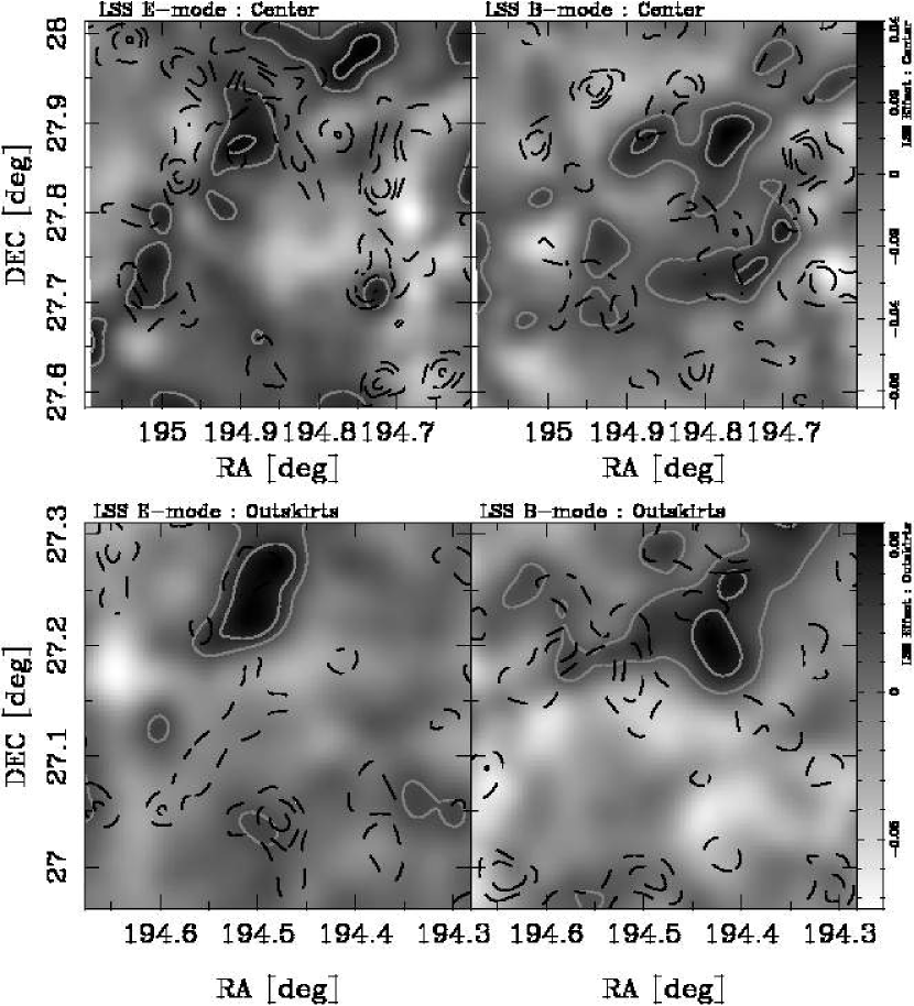
Figure 7.— The E- and B-mode maps reconstructed by background LSS model alone. Top-left : E-mode map in central region. Top-right : B-mode map in central region. Bottom-left : E-mode map in outskirts. Bottom-right: B-mode map in outskirts. The box sizes and contour scales are the same as those in Figure 2 and 3. Gray solid and black dashed lines show contours derived from LSS and observed shears, respectively. There are three LSS structures with a size of a few arcmins at a $\sim 2\sigma$ level. In particular, the LSS convergences at a $\sim 1\sigma$ level are found in the clump candidates 5 and 8.

5. Projected Mass Measurements for Subclumps

We measure projected mass of subclump candidates (labeled in Figures 2 and 3) which are identified above the $3\sigma$ significant level in the mass map. The projected masses, $M_{\rm\zeta_{c}}(<\theta)$, are estimated by the so-called $\zeta_{c}$-statistics (Clowe et al. 2000) which is modified version of original one (Fahlman et al. 1994),

$$M_{\rm\zeta_{c}}(<\theta)=\pi{\theta}^{2}\Sigma_{\rm cr}\zeta_{c}(\theta,\theta_{{\rm b1}},\theta_{{\rm b2}}),$$ (5)

where,

$$\zeta_{c}(\theta,\theta_{{\rm b1}},\theta_{{\rm b2}}) \equiv 2\int_{\theta}^{\theta_{{\rm b1}}}\!d\ln\theta~{}\langle\gamma_{+}\rangle(\theta)$$ (6)

$$+\frac{2}{1-\theta_{{\rm b1}}^{2}/\theta_{{\rm b2}}^{2}}\int^{\theta_{{\rm b2}}}_{\theta_{{\rm b1}}}\!d\ln\theta~{}\langle\gamma_{+}\rangle(\theta)$$

$$= \bar{\kappa}(<\theta)-\bar{\kappa}(\theta_{{\rm b1}}\leq\theta\leq\theta_{{\rm b2}}).$$

Here, $\theta$ is a given radius and, $\theta_{{\rm b1}}$ and $\theta_{{\rm b2}}$ are the inner and outer radii of subtracted background region. The critical surface density $\Sigma_{\rm cr}=c^{2}/(4\pi G)(D_{\rm s}{D_{\rm ls}/D_{\rm l}})$ is given by the angular diameter distances to cluster ($D_{\rm l}$), to source ($D_{\rm s}$) and between cluster and source ($D_{\rm ls}$). The $M_{\zeta_{c}}$ is a model-independent mass estimation.

We first obtain central positions of mass clumps by peak-finding algorithms and then redistribute them within $0\farcm 2$ over 500 Monte Carlo simulations to take into account uncertainties of central positions. We choice the central position at which the signal-to-nose ratio of $\zeta_{c}$ measurement is at the maximum (Table 3). The background region is in the annulus of $40-100$kpc surrounding candidates so that we extract the substructure mass embedded in the cluster main potential. If the cluster potential is uniform within $\sim 100$kpc, it is a good mass estimate of subclumps. The following results are not changed by choosing the background region. As described in eq. (6), $\zeta_{c}$ mass measurement is computed by integrating the measured tangential shears outside a given radius $\theta$. Since the available number for background galaxies in the outer annulus is larger than those in the inner one, it enables us to plot $M_{\zeta_{c}}$ profile for each mass clump.

We also calculate LSS-corrected projected masses, $M_{\zeta_{\rm c}}^{\rm(corr)}$, in terms of $\langle\gamma_{+}\rangle(\theta)-\langle\gamma_{+}^{\rm(LSS)}\rangle(\theta)$, where $\gamma_{+}^{\rm(LSS)}$ is the LSS shears obtained in §4.4. We do not consider the intrinsic shape noise. We note that $M_{\zeta_{\rm c}}^{\rm(corr)}$ is a model-dependent mass because we assumed the mass-to-light ratio in a calculation of LSS shears, $\gamma_{\alpha}^{\rm(LSS)}$. Figure 8 shows the LSS-uncorrected and corrected projected mass profiles, respectively. The values of $M_{\zeta_{c}}$ are saturated on the outer radius, which indicates that the mass density of clumps is quite low on the outer radius. We estimate two-dimensional masses for each clump, $M_{\rm 2D}$ and $M_{\rm 2D}^{\rm(corr)}$, from the saturated values with a covariance matrix, because each bin is correlated with each other. We list the resulting masses in Table 3. The LSS- uncorrected and corrected masses are in good agreement with each other, but for candidate 5. The LSS-corrected mass for candidate 5 is about half of that before a correction. Therefore, the background LSS effect significantly contributes on lensing signals for candidate 5.

The mean values are $\langle M_{{\rm 2D}}^{\rm(corr)}\rangle=(4.84\pm 1.41)\times 10^{12}h^{-1}M_{\sun}$ for all candidates and $\langle M_{{\rm 2D}}^{\rm(corr)}\rangle=(5.06\pm 1.30)\times 10^{12}h^{-1}M_{\sun}$ but for candidate 5. They are at the order of the mass of cD galaxy halos, $M_{{\rm 3D}}^{\rm(SIS)}(\theta)=3.0\times 10^{12}h^{-1}M_{\sun}(\sigma_{v}/400{\rm km/s})^{2}(r/40{\rm kpc})$, where $\sigma_{v}$ is the velocity dispersion and we employ the velocity dispersion of cD galaxy $\sim 200-400{\rm km/s}$ (e.g. Smith et al. 2000). Although we looked into the SDSS photometric and spectroscopic data, there is no correlation among the projected mass, and velocity dispersion and luminosity of galaxies which are located in each subclump.

Table 3Projected Mass for Subclump candidates

ID	S/N	$\nu$	$P_{\rm spur}$	$b_{\rm map}$	$M_{\rm 2D}$	$M_{\rm 2D}^{\rm(corr)}$	(RA, Dec)	Name	$d_{\rm off}$
			$\%$		$10^{12}h^{-1}M_{\sun}$	$10^{12}h^{-1}M_{\sun}$	deg		arcmin
(1)	(2)	(3)	(4)	(5)	(6)	(7)	(8)	(9)	(10)
1	$3.1$	$3.6$	$0.0$	$0.0$	$8.01\pm 1.05$	$7.70\pm 1.05$	$(195.042,27.996)$	NGC 4889	$1.2$
2	$3.9$	$3.7$	-	-	$4.28\pm 0.83$	$4.56\pm 0.83$	$(194.882,27.948)$	NGC 4874	$1.2$
3	$3.2$	$2.9$	$0.4$	$1.3$	$5.03\pm 0.87$	$5.29\pm 0.87$	$(194.980,27.843)$	SA 1656-054	$1.2$
4	$3.6$	$3.2$	$0.0$	$0.0$	$3.49\pm 0.74$	$3.73\pm 0.74$	$(194.722,27.829)$	SDSS J125848.72+274837.5	$0.7$
5	$3.4$	$3.1$	$12.2$	$41.1$	$5.95\pm 1.08$	$2.74\pm 1.08$	$(194.732,27.722)$	-	-
6	$3.3$	$3.1$	$0.3$	$1.0$	$4.63\pm 0.84$	$4.54\pm 0.84$	$(194.724,27.612)$	SDSS J125858.10+273540.9	$1.4$
7	$3.1$	$3.1$	$0.1$	$0.3$	$6.07\pm 1.24$	$7.32\pm 1.24$	$(194.643,27.625)$	NGC 4853	$1.7$
8	$3.3$	$3.4$	$1.8$	$8.2$	$5.90\pm 1.32$	$4.61\pm 1.32$	$(194.475,27.044)$	SDSS J125756.65+270215.0	$0.8$

Figure 8.— Aperture mass profile, $M_{\zeta_{c}}$, for each subclump candidate (1-8). Open and filled circles represent aperture masses without and with LSS correction, respectively. Aperture masses are saturated on the outer radii, which indicates that the mass density in the surroundings are quite low. It is consistent with results of stacked lensing analysis (§6). The aperture mass for candidate 5, corrected by LSS lensing effect, reduces to about half of that without a LSS correction.

6. Tangential Shear Profile Stacked Over Five Subclumps

Since weak lensing signals of Coma cluster at the low redshift is weak and the number of background galaxies within small radius is few, it is quite difficult to measure tangential shear profile for each subclump candidate. We therefore measure a profile of tangential shear components ensembling five subclump candidates. A mass measurement with stacked tangential distortion profile is complementary to the $\zeta_{c}$ statistics (§5), because different shear catalogue is used in two measurements. In the $\zeta_{c}$ statistics, source galaxies outside a given radius is used, while, in the tangential shear measurement, source galaxies from inner to outer radius is independently available. We here exclude two dark halos associated with cD galaxies in order to avoid a contamination of lensing distortion caused by the main cluster. The candidate 5 at which the projection effect is significant is also ignored. The center for each subclump is chosen as the same position of the $M_{\zeta_{c}}$ measurements (§5). The averaged tangential shear distortions of source galaxies, $\langle g_{+}\rangle(\theta_{n})$, is calculated in the circular annulus of the same radius, based on the same procedure as §3. The typical projected distance between a center of a stacked tangential shear profile and the main cluster center, $\langle\theta_{{\rm off}}\rangle$, is obtained with a weight function of lensing signals, $\langle\theta_{{\rm off}}\rangle^{2}=\sum_{j}\langle g_{+,j}\rangle^{2}\theta_{{\rm off},j}^{2}/\sum_{j}\langle g_{+,j}\rangle^{2}\sim 17\farcm 4$, where $\langle g_{+,j}\rangle$ is the lensing signal (§3) for each subclump and $\theta_{{\rm off},j}$ is an angular separation between each subclump and the main center.

We compute the LSS-corrected shear profile, $\langle g_{+}\rangle(\theta_{n})-\langle g_{+}^{\rm(LSS)}\rangle(\theta_{n})$, where the azimuthal average of the LSS distortion components, $\langle g_{+}^{\rm(LSS)}\rangle(\theta_{n})$, are calculated without statistical weight ($u_{g,i}=1$). Figure 9 shows the stacked tangential shear profiles as a function of transverse separation $\theta$, with and without the LSS effect. We estimate the contribution of the main cluster mass on the stacked lensing signals, because the tangential shear provides full information on the lensing signals of gravitational potentials of both the main cluster and subclumps. It is necessary to calculate lensing distortions caused by the main cluster in order to measure typical mass of interior subhalos. We follow the convolution technique of Yang et al. (2006) to measure the azimuthally averaged convergence at the offset from the main cluster center in the lens plane. The values of $g_{+}$ of the offset main halo is at the order of ${\it O}(-10^{-5})$ in the range of the stacked lensing profile ($\theta<6\farcm$), which indicates that the lensing signals from the main cluster at the positions of subclumps are negligible.

Since the tidal field of main cluster disrupts dark matter halos of interior substructures, the subhalo radius would be determined by the tidal radius rather than the virial radius $r_{\rm vir}$. We therefore consider a truncated SIS model (TSIS) and a truncated NFW model (TNFW) for the tangential fitting, whose density profiles are truncated at the radius $r_{t}$.

$$\rho_{\rm TSIS}(r) = \frac{\sigma_{v,t}^{2}}{2\pi Gr^{2}}~{}~{}~{}~{}{\rm for}~{}~{}r\leq r_{t}$$

$$= 0~{}~{}~{}~{}~{}~{}~{}~{}~{}~{}~{}{\rm for}~{}~{}r>r_{t}$$

$$\rho_{\rm TNFW}(r) = \frac{M_{\rm sub}^{\rm(TNFW)}}{4\pi r_{s,t}^{3}m(c_{t})}\frac{1}{(r/r_{s,t})(1+r/r_{s,t})^{2}}~{}~{}~{}{\rm for}~{}~{}r\leq r_{t}$$ (8)

$$= 0~{}~{}~{}~{}~{}~{}~{}~{}~{}~{}~{}~{}~{}~{}~{}~{}~{}~{}~{}~{}~{}~{}~{}~{}~{}~{}~{}~{}~{}~{}~{}~{}~{}~{}~{}{\rm for}~{}~{}r>r_{t},$$

where $\sigma_{v,t}^{2}$ is a velocity dispersion for TSIS model, $M_{{\rm sub}}^{\rm(TNFW)}$ and $c_{t}$ are a mass and a concentration for TNFW model, and $r_{s,t}=r_{t}/c_{t}$ is a scale radius determined by the concentration and the truncated radius $r_{t}$. The subclump mass for TSIS model is given by $M_{\rm sub}^{\rm(TSIS)}=2\sigma_{v,t}^{2}r_{t}/G$.

Analytical expressions of the two-dimensional projection $\Sigma$ of the density field are obtained by an integration over $r_{\parallel}=[-\sqrt{r_{t}^{2}-r^{2}},+\sqrt{r_{t}^{2}-r^{2}}]$

$$\kappa_{\rm TSIS}(\theta) = \left\{\begin{array}[]{ll}\frac{1}{\pi}\left(\frac{\theta_{E,t}}{\theta}\right)\arccos\left(\frac{\theta}{\theta_{t}}\right)&~{}~{}{\rm for}~{}~{}\theta\leq\theta_{t}\\ 0&~{}~{}{\rm for}~{}~{}\theta>\theta_{t}\end{array}\right.$$ (10)

where $\theta=r/D_{l}$ is an angular size of the three dimensional radius, and $\theta_{E,t}\equiv 4\pi(\sigma_{v,t}/c)^{2}D_{\rm ls}/D_{\rm s}$ is the Einstein radius for TSIS model.

$$\kappa_{\rm TNFW}(\theta) = \frac{M_{\rm sub}^{\rm(TNFW)}}{2\pi\Sigma_{\rm cr}r_{s,t}^{2}m(c_{t})}f(x),~{}~{}~{}~{}x=\theta/\theta_{s,t}$$ (11)

$$f(x) = \left\{\begin{array}[]{l}-\frac{\sqrt{c_{t}^{2}-x^{2}}}{(1-x^{2})(1+c_{t})}+\frac{1}{(1-x^{2})^{3/2}}{\rm arccosh}\left(\frac{x^{2}+c_{t}}{x(1+c_{t})}\right)\\ {\rm~{}~{}~{}~{}~{}~{}~{}~{}~{}~{}~{}~{}~{}~{}~{}~{}~{}~{}~{}~{}~{}~{}~{}~{}~{}~{}~{}~{}~{}~{}for}~{}~{}x<1\\ \frac{\sqrt{c_{t}^{2}-1}}{3(1+c_{t})}\left(1+\frac{1}{1+c_{t}}\right)\\ {\rm~{}~{}~{}~{}~{}~{}~{}~{}~{}~{}~{}~{}~{}~{}~{}~{}~{}~{}~{}~{}~{}~{}~{}~{}~{}~{}~{}~{}~{}~{}for}~{}~{}x=1\\ -\frac{\sqrt{c_{t}^{2}-x^{2}}}{(1-x^{2})(1+c_{t})}-\frac{1}{(x^{2}-1)^{3/2}}{\rm arccos}\left(\frac{x^{2}+c_{t}}{x(1+c_{t})}\right)\\ {\rm~{}~{}~{}~{}~{}~{}~{}~{}~{}~{}~{}~{}~{}~{}~{}~{}~{}~{}~{}~{}~{}~{}~{}~{}~{}~{}~{}~{}~{}~{}for}~{}~{}1<x\leq c_{t}\\ 0\\ {\rm~{}~{}~{}~{}~{}~{}~{}~{}~{}~{}~{}~{}~{}~{}~{}~{}~{}~{}~{}~{}~{}~{}~{}~{}~{}~{}~{}~{}~{}~{}for}~{}~{}c_{t}<x\end{array}\right.$$ (20)

The expression of $f(x)$ is the same as Takada & Jain (2003) and Hamana, Takada & Yoshida (2004), although they adopt that the mass density is truncated at the virial radius. We here do not assume $r_{t}=r_{\rm vir}$, because we aim to investigate disrupted interior substructures. The TSIS and TNFW profiles are specified in terms of two parameters of $\theta_{E,t}$ and $\theta_{t}$ and three parameters of $M_{\rm sub}^{\rm(TNFW)}$, $c_{t}$ and $\theta_{t}$, respectively.

We fit the LSS- uncorrected and corrected distortion profiles with TSIS and TNFW models. The best-fit parameters are summarized in Table 4. Two models well describe the stacked tangential shear profile. The best-fit parameters with and without a LSS lensing correction does not change significantly. The truncated radii for two models are in good agreements with each other. Indeed, the break in the tangential shear profile is clearly found at $\theta\sim 1\farcm 75$ (Figure 9). The values of $g_{+}$ steeply decrease ($\propto\theta^{-2}$) over the truncated radius, which indicates that the halo mass density drops to zero at the truncated radius. It is consistent with the $\zeta_{\rm c}$ mass measurement (§5). This feature does not clearly appear in a stacked lens analysis for massive clusters of $M_{\rm vir}>10^{14}h^{-1}M_{\sun}$ (Okabe et al. 2009). The TNFW and TSIS masses are in agreements with the the mean projected mass $\langle M_{\rm 2D}^{\rm(corr)}\rangle_{34678}=(4.78\pm 1.07)\times 10^{12}h^{-1}M_{\sun}$. We note that the two-dimensional mass for truncated mass models (TNFW and TSIS) has the same analytical expression as the three-dimensional mass ($M_{\rm 2D}^{{\rm TSIS}}=M_{\rm 3D}^{{\rm TSIS}}$ and $M_{\rm 2D}^{{\rm TNFW}}=M_{\rm 3D}^{{\rm TNFW}}$), because there is no projection effect due to the zero mass outside $r_{t}$.

We also investigate model fittings for spurious mass clumps appeared in mass maps simulated by rotated shear catalogue. First, we randomly rotate an angle in the ($g_{1},g_{2}$) plane for each background galaxies with it’s $|g|$ fixed and then conduct the mass reconstruction for background catalogue by 500 times. Second, we detect peaks whose significance is over $3\sigma$ in mass maps. Third, we measure stacked tangential profiles for 5 peaks which are bootstrap re-sampled from detected peaks by 300 times. In the measurements, the peak whose distance from cluster center is more than $10\farcm$ is only used in order to avoid the main cluster lensing signal (Yang et al. 2006). The averaged $\chi^{2}$s are $\langle\chi^{2}\rangle=9.9$ for TNFW and $\langle\chi^{2}\rangle=15.7$ for TSIS models. Those $\chi^{2}$s are worse than our results. This is why the form of stacked tangential profile for spurious clumps is different from Figure 9.

Figure 9.— Profiles of tangential shear component (top panel), $g_{+}$, and the $45$ degree rotated component (bottom panel), $g_{\times}$, obtained from an ensemble of five subclumps. Left : the stacked profile from original shear catalogue. Right : the profile with a LSS lensing correction. The $g_{+}$ values clearly decrease over $\theta\sim 1\farcm 75$. The solid and dashed lines are subhalo models of TSIS and TNFW, respectively.

Table 4The best-fit truncated SIS (TSIS) and truncated NFW (TNFW) model parameters.

TSIS	LSS uncorrected	LSS corrected
(1)	(2)	(3)
$M_{\rm sub}^{\rm(TSIS)}$ [$10^{12}h^{-1}M_{\sun}$]	$3.47_{-0.56}^{+1.21}$	$3.54_{-0.54}^{+1.32}$
$\theta_{t}$ [arcmin]	$1.76_{-0.15}^{+0.57}$	$1.76_{-0.13}^{+0.61}$
$r_{t}$ [$h^{-1}{\rm kpc}$]	$35.21_{-2.98}^{+11.32}$	$35.21_{-2.58}^{+12.25}$
$\sigma_{v,t}$ [km/s]	$460.59_{-32.70}^{+30.53}$	$465.27_{-32.31}^{+30.21}$
$\chi^{2}/{\rm d.o.f}$	$4.4/7$	$5.3/7$
TNFW	LSS uncorrected	LSS corrected
(4)	(5)	(6)
$M_{\rm sub}^{\rm(TNFW)}$ [$10^{12}h^{-1}M_{\sun}$]	$3.90_{-0.47}^{+1.22}$	$4.00_{-0.37}^{+1.45}$
$\theta_{t}$ [arcmin]	$1.75_{-0.26}^{+0.25}$	$1.75_{-0.29}^{+0.21}$
$r_{t}$ [$h^{-1}{\rm kpc}$]	$35.01_{-5.28}^{+4.99}$	$35.01_{-5.79}^{+4.21}$
$c_{t}$	$1.53_{-0.79}^{+1.12}$	$1.53_{-0.68}^{+0.74}$
$\chi^{2}/{\rm d.o.f}$	$2.5/6$	$2.4/6$

7. Discussion and Conclusion

7.1. Cluster Mass Comparison

We compare our mass estimates with previous results of multi-wavelength data. The line-of-sight velocity distribution of member galaxies with the Jeans equation which requires the assumption of the dynamical equilibrium derived $M_{\rm vir}=9.8\times 10^{14}h^{-1}M_{\sun}$ and $c_{\rm vir}=9.4$ for NFW mass model (Łokas & Mamon 2003). The caustic mass estimates to use a characteristic pattern in the redshift-space, formed by galaxies falling into cluster potential (Kaiser 1987) obtained $M_{\rm 200}=7.85\times 10^{14}h^{-1}M_{\sun}$ and $c_{200}=10$ (Rines et al. 2003). Our result of NFW mass $M_{\rm vir}$ and $M_{\rm 200}$ is in good agreement with their results, while our concentration parameter is lower. Our weak lensing analysis is to use one band imaging data. As demonstrated by Broadhurst et al. (2005), see also ( Umetsu & Broadhurst 2008 ; Okabe et al. 2009), the dilution contamination of member galaxies on lensing signals is problematic for an accurate measurement of the concentration parameter. It is therefore of importance to correct the dilution effect by secure selecting of background galaxies in the color-magnitude plane (Broadhurst et al. 2005; Umetsu & Broadhurst 2008; Umetsu et al. 2009). In addition, we require the data, which covers the virial radius, in order to improve measurement accuracy of halo mass. The SDSS and CHFT weak lensing results (Kubo et al. 2007; Gavazzi et al. 2009) are $M_{200}=18.8^{+6.5}_{-5.6}\times 10^{14}M_{\sun}$ and $M_{200}=5.1^{+4.3}_{-2.1}\times 10^{14}M_{\sun}$, and $c_{200}=3.84^{+13.16}_{-0.18}$ and $c_{200}=5.0^{+3.2}_{-2.5}$. They do not disagree with our results within large errors. The ASCA and ROSAT X-ray observations with assumptions of hydrostatic equilibrium, isothermally and single $\beta$ model shows $M_{500}=11.99^{+1.28}_{-1.29}\times 10^{14}M_{\sun}$ (Reiprich & Böhringer 2002) and $M_{500}=9.95^{+2.10}_{-2.99}\times 10^{14}M_{\sun}$ (Chen et al. 2007), which are higher than our estimates. We cannot rule out a possibility that the low angular resolution of ASCA satellite leads to a bias on mass estimates. It is of critical importance to compare X-ray and weak-lensing masses of Coma cluster which is the only cluster known to have turbulence in the ICM. The ASCA and XMM-Newton X-ray observations (e.g. Watanabe et al. 1999; Arnaud et al. 2001) have shown the complex temperature variations in the intra-cluster medium (ICM). Schuecker et al. (2004) has revealed a Kolmogorov/Oboukhov-type turbulence spectrum in the ICM as a consequence of the projected pressure distributions. They constrained that the lower limit of turbulent pressure accounts for 10 percent of the total ICM pressure. Recent hydrodynamic N-body simulations pointed out that X-ray mass estimates with an assumption of hydrostatic equilibrium are biased low due to ICM turbulence, because the gas motion pressure of turbulence as well as bulk motions supports a part of the total pressure (e.g. Ervard et al. 1999; Nagai et al. 2007). Their results cast a doubt on accurate cluster mass measurement by X-ray analysis alone, which is a serious concern for cluster-based cosmological probes (e.g. Vikhlinin et al. 2009a,b; Okabe et al. 2010; Zhang et al. 2010). Therefore, a comparison of independent mass estimates is of great importance to understand, in a quantitative manner, how much the gas motion pressure affects the X-ray mass estimates.

7.2. Comparison with X-ray image

We compare an X-ray exposure-corrected image retrieved from archival data of XMM-Newton with mass counters of the central region (Figure 10). The XMM-Newton data in the outskirts region is lacked. The X-ray image shows some point sources associated with galaxies in clump candidates. The intra-cluster-medium (ICM) distributions are not correlated with mass clump candidates. This is why the intra-cluster plasma can be escaped from the gravitational potential of subclumps. The sound velocity of the ICM is given by

$$c_{s}=\left(\frac{5k_{B}T}{3\mu m_{p}}\right)^{1/2}\simeq 1457\left(\frac{k_{B}T}{8.25{\rm keV}}\right)^{1/2}{\rm km/s},$$ (21)

where the temperature $k_{B}T=8.25\pm 0.10$keV (Arnaud, et al. 2001), the mean molecular weight $\mu=0.62$, and the proton mass $m_{p}$. The sound velocity is higher than the typical escape velocity from subclumps, as below

$$c_{s}\geq v_{\rm esc}=\left(\frac{2GM_{\rm sub}^{\rm(TNFW)}}{r_{t}}\right)^{1/2}\simeq 991{\rm km/s}.$$ (22)

Since the temperature of point sources is low $k_{B}T\sim 1{\rm keV}$ and high metal abundance (Vikhlinin et al. 2001), it’s sound velocity is lower than the escape velocity.

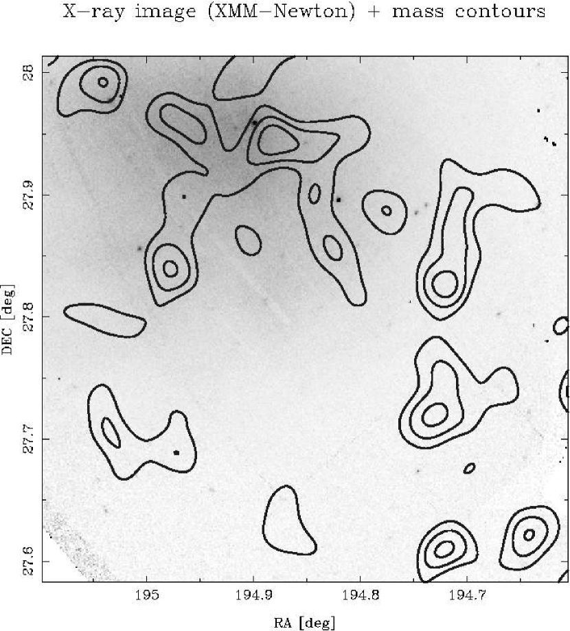
Figure 10.— X-ray exposure-corrected image, no-subtracted backgrounds, overlaid with mass contours of the central $26\farcm\times 26\farcm$ cluster region.

.

7.3. Tidal Radius

The stacked tangential shear profile for five subclumps, excluding subhalos associated with cD galaxies and candidate 5, is well described by the TSIS and TNFW models. The fitting result gives the truncated radius $r_{t}\simeq 35h^{-1}~{}{\rm kpc}$, which coincides with galaxy-galaxy lensing results in clusters (e.g. Natarajan & Springel 2004; Natarajan, De Lucia & Springel 2007). The truncated radius is much smaller than a truncated radius $\sim 200~{}{\rm kpc}$ obtained by galaxy-galaxy lensing studies of fields (e.g. Hoekstra, Yee & Gladders 2004). It would be due to the strong tidal field of the main cluster gravitational potential. The tidal radius of a subhalo orbiting in a spherically, symmetric mass distribution of a cluster is obtained by the balance between the tidal force of the primary halo and the gravity of subclump, $r_{\rm tidal}=(M_{\rm sub}/(M(<r_{p})(2-\partial\log M/\partial\log r_{p}))^{1/3}r_{p}$ (e.g. Tormen et al. 1998), where $r_{p}$ is the pericenter radius which is the minimal radius from the cluster center during its orbiting history. Since we do not constrain its pericenter radius directly from a current position and not derive the three-dimensional radius, we instead assume the mean, projected offset radius $\langle\theta_{\rm off}\rangle$ of subclumps in stacked lensing analysis. Here, we assume the NFW and TNFW mass models for the main cluster and substructures, respectively. We obtain the tidal radius $r_{\rm tidal}\sim 42~{}h^{-1}{\rm kpc}$, which coincides with the truncated radius $r_{t}\simeq 35~{}h^{-1}{\rm kpc}$.

7.4. Subhalo Mass Fraction

We found four subhalos and two cD galaxy halos in the central data ($r\lower 2.15277pt\hbox{$\;\buildrel<\over{\sim}\;$}30\farcm$) and one halo in the outskirts data ($30\farcm\lower 2.15277pt\hbox{$\;\buildrel<\over{\sim}\;$}r\lower 2.15277pt\hbox{$\;\buildrel<\over{\sim}\;$}60\farcm$). There is a difference of the halo number for the radius, which might support the results of numerical simulation (e.g De Lucia et al. 2004;Gao et al 2004) that the number of substructure increases as the radius decreases. Compensating the limitation of our data region, we roughly estimate the number of subhalos within the radii $r_{\rm vir}$ and $r_{200}$. If we assume that there are four ($r\lower 2.15277pt\hbox{$\;\buildrel<\over{\sim}\;$}30\farcm$) and one ($30\farcm\lower 2.15277pt\hbox{$\;\buildrel<\over{\sim}\;$}r\lower 2.15277pt\hbox{$\;\buildrel<\over{\sim}\;$}60\farcm$) subhalos in the area corresponding to our data, the halo number is estimated to be $\pi(r_{\rm vir}^{2}-30\farcm^{2})/A_{\rm outskirts}+4\times(\pi 30\farcm^{2}/A_{\rm center})+2{\rm cDs}$, where $A$ is the area of our data. The Poisson noise for distributions is applied for the statistical errors.

The halo number detected by weak lensing analysis is expected to be $N_{\rm sub}(<r_{\rm vir})=43\pm 30$ and $N_{\rm sub}(<r_{\rm 200})=27\pm 15$. If the typical halo mass is the best-fit value $\langle M_{\rm sub}^{\rm(TNFW)}\rangle=4.00\times 10^{12}h^{-1}M_{\sun}$ obtained from fitting of the stacked tangential profile, the total substructure mass within the virial radius account for $\sim 19\pm 13$ and $17\pm 9$ percents of total cluster masses $M_{\rm vir}$ and $M_{200}$, respectively. Although the total mass fraction contained in subhalos does not agree each other among literature (e.g. De Lucia et al. 2004; Natarajan, De Lucia & Springel 2007, Gao et al. 2004), most authors estimate 5 -20 percent. Our result is in rough agreement with the numerical simulations. A galaxy-galaxy lensing study (Natarajan, De Lucia & Springel 2007) indicates that $10-20\%$ of the mass is contained in cluster substructures, which also roughly agrees with our result.

Our weak lensing analysis on the nearby cluster would indicate the possibility that the mass function of cluster substructures is measurable without assumptions of mass-to-light ratio for member galaxies and dynamical state, while the galaxy-galaxy lensing studies (e.g. Natarajan & Springel 2004; Natarajan, De Lucia & Springel 2007) requires the assumption of the mass and light scaling law. We however have not yet obtained the mass spectrum as the galaxy-galaxy lensing studies (e.g. Natarajan & Springel 2004; Natarajan, De Lucia & Springel 2007).

Alternative possible approach to investigate the mass function of cluster substructures is to measure higher order moments of the lensed images (HOLICs) and using the moments to estimate the flexion (e.g. Okura et al. 2007; Okura & Futamase 2008; Okura et al. 2008). They have shown for the first time that flexion analysis can discover substructures using the image of A1689 (Okura et al. 2007).

As pointed out by Shaw et al. (2006), the median mass fraction is a increase function of the virial mass ($f_{\rm sub}\propto M_{\rm vir}^{0.44\pm 0.06}$), because massive objects, which formed more recently than less massive objects, have less time to disrupt subhalos (Zenter et al. 2005). The statistical study of mass fraction of galaxy clusters is, therefore, one of good tests of $\Lambda$CDM and the hierarchical clustering, as the concentration-mass relation of the NFW mass model (Okabe et al. 2009). Hence, further systematic study of mass fractions is required.

The area of our current data is insufficient to derive the halo mass function as well as to measure cluster mass accurately. The next instrument of a prime focus camera of Subaru telescope, Hyper-Suprime-Cam, whose field-of-view is $\sim 1.5{\rm deg^{2}}$, will efficiently observe the nearby cluster and enables us to conduct weak lensing and flexion analyses. Our result using the Subaru/Suprime-Cam does guarantee that weak lensing analysis using Subaru/Suprime-Cam and Hyper-Suprime-Cam is capable for almost X-ray clusters.

References

- Abazajian et al. (2009) Abazajian, K., N., et al. 2009, ApJS, 182, 543.
- Arnaud, et al. (2001) Arnaud, M. et al. 2001, A&A, 365, L67.
- Broadhurst et al. (2005) Broadhurst, T., Takada, M., Umetsu, K., et al., 2005, ApJL, 619, 143.
- Chen et al. (2007) Chen, Y., Reiprich, T. H., Böhringer, H., Ikebe, Y., Zhang, Y.-Y. 2007, A&A, 466, 805.
- Conselice & Gallagher (1999) Conselice, C., J.& Gallagher, J., S., III, 1999, AJ, 117, 75.
- Clowe et al. (2000) Clowe, D., Luppino, G. A., Kaiser, N., & Gioia, I. M., 2000, ApJ, 539, 540.
- De Lucia et al. (2004) De Lucia, G., Kauffmann, G., Springel, V., White, S. D. M., Lanzoni, B., Stoehr, F., Tormen, G. & Yoshida, N. 2004, MNRAS, 348, 333.
- Duffy et al. (2008) Duffy, A., R., Schaye, J., Kay., Scott T., & Dalla V., C., 2008,MNRAS, 390, L64.
- Erben et al. (2001) Erben, T., van Waerbeke, L., Bertin, E., Mellier, Y., & Schneider, P. 2001, A&A, 366, 717.
- Evrard et al. (1996) Evrard, A., E., Metzler, C., A., & Navarro, J., F., 1996, ApJ, 469, 494.
- Fahlman et al. (1994) Fahlman, G., Kaiser, N., Squires G. & Woods, D. 1994, ApJ, 437, 56.
- Gao et al. (2004) Gao, L., White, S. D. M., Jenkins, A., Stoehr, F. & Springel, V., 2004, MNRAS, 355, 819.
- (13) Gavazzi, R., Adami, C., Durret, F., Cuillandre, J.-C., Ilbert, O., Mazure, A. & Pelló, R.,& Ulmer, M., P., 2009,A&A, 498, L33.
- Guzik & Seljak (2002) Guzik, J. & Seljak, U. 2002, MNRAS, 335,311.
- Hamana, Takada & Yoshida (2004) Hamana, T., Takada, M. & Yoshida, N., 2004, MNRAS, 350, 893.
- Hoekstra et al. (2004) Hoekstra, H., Yee, H. K. C. & Gladders, M. D. 2004, ApJ, 606, 67.
- Hoekstra et al. (2005) Hoekstra, H., Hsieh, B., C., Yee, H., K., C., Lin, H., & Gladders, M., D., 2005, ApJ, 635, 73.
- Johnston et al. (2007) Johnston, D., E., Sheldon, E., S., Wechsler, R., H., Rozo, E., Koester, B., P., Frieman, J., A., McKay, T., A., Evrard, A., E., Becker, M., R.; Annis, J., 2007, arXiv0709.1159.
- Kaiser (1987) Kaiser, N. 1987, MNRAS, 227, 1.
- Kaiser & Squires (1993) Kaiser, N. & Squires, G. 1993, ApJ, 404, 441.
- Kaiser, Squires & Broadhurst (1995) Kaiser, N., Squires, G., Broadhurst, T., 1995, ApJ, 449, 460.
- Koester et al. (2007) Koester et al. 2007, ApJ, 660, 239.
- Kubo et al. (2007) Kubo, J., M., Stebbins, A., Annis, J., Dell’Antonio, I., P., Lin, H., Khiabanian, H., Frieman, J. A., 2007, ApJ, 671, 1466.
- (24) Łokas, E., L., & Mamon, G., A., 2003, MNRAS,343, 401.
- Mandelbaum et al. (2005) Mandelbaum, R., Tasitsiomi, A., Seljak, U., Kravtsov, A. V. & Wechsler, R. H., 2005, MNRAS, 362, 1451.
- Miyazaki et al. (2002) Miyazaki, S. et al. 2002, PASJ, 54, 833,801.
- Miyazaki et al. (2007) Miyazaki, S. et al. 2007,ApJ, 669, 714.
- Nakamura & Suto (1997) Nakamura, T. T. & Suto, Y. 1997, Progress of Theoretical Physics, 97, 49.
- Natarajan & Springel (2004) Natarajan, P. & Springel, V., 2004, ApJ, 617,L13.
- Natarajan, De Lucia & Springel (2007) Natarajan, P., De Lucia, G. & Springel, V. 2007, MNRAS, 376, 180.
- Nagai et al. (2007) Nagai, D., Vikhlinin, A., & Kravtsov, A. V. 2007, ApJ, 655, 98.
- Navarro, Frenk, & White (1996) Navarro, J. F.,Frenk, C. S. & White, S. D. M. 1996, ApJ, 462, 563.
- Ouchi et al. (2004) Ouchi, M., et al. 2004, ApJ, 611, 660.
- Okabe & Umetsu (2008) Okabe, N. & Umetsu, K. 2008, PASJ, 60, 345.
- Okabe et al. (2009) Okabe, N., Takada, M., Umetsu, K., Futamase, T., & Smith, G., P., 2008, PASJ, submitted, arXiv:0903.1103
- Okabe et al. (2010) Okabe, N., Zhang, Y.-Y., Finoguenov, A., et al. 2010, ApJ, submitted
- Okura et al. (2007) Okura, Y., Umetsu, K. & Futamase, T. 2007, ApJ, 660, 995.
- Okura & Futamase (2008) Okura, Y. & Futamase, T., 2008, arXiv0805.4498O.
- Okura et al. (2008) Okura, Y., Umetsu, K. & Futamase, T. 2008, ApJ, 680, 10.
- Oyaizu et al. (2008) Oyaizu, H., Lima, M., Cunha, C., E., Lin, H., Frieman, J. & Sheldon, E., S., 2008, ApJ, 674, 768.
- Reiprich & Bö hringer (2002) Reiprich, T., H., & Bö hringer, H. 2002,ApJ, 567, 716.
- Rines et al. (2003) Rines, K., Geller, M., J., Kurtz, M., J., & Diaferio, A., 2003, AJ, 126, 2152.
- Seljak (2000) Seljak, U. 2000, MNRAS, 318, 203.
- Shaw et al. (2006) Shaw, L., D., Weller, J., Ostriker, J. P.& Bode, P. 2006, ApJ, 646, 815.
- Schuecker et al. (2004) Schuecker, P., Finoguenov, A., Miniati, F., Bö hringer, H. & Briel, U., G., 2004, A&A, 426, 387.
- Smith et al. (2000) Smith, R. J., Lucey, J. R., Hudson, M., J., Schlegel, D., J., & Davies, R. L., 2000, MNRAS, 313, 469.
- Takada & Jain (2003) Takada, M. & Jain, B. 2003, MNRAS,340, 580.
- Tormen et al. (1998) Tormen, G., Diaferio, A., & Syer, D., 1998,MNRAS, 299, 728.
- Umetsu & Broadhurst (2008) Umetsu, K. & Broadhurst, T., 2008, ApJ, 684, 177.
- Umetsu et al. (2009) Umetsu, K. et al. 2009, arXiv:0908.0069.
- Vikhlinin et al. (2001) Vikhlinin, A., Markevitch, M., Forman, W. & Jones, C.,2001, ApJ, 555, L87.
- Vikhlinin et al. (2009a) Vikhlinin, A., Burenin, R. A., Ebeling, H., et al. 2009a, ApJ, 692, 1033
- Vikhlinin et al. (2009b) Vikhlinin, A., Kravtsov, A. V., Burenin, R. A., et al. 2009b, ApJ, 692, 1060
- Watanabe et al. (1999) Watanabe, M., Yamashita, K., Furuzawa, A., Kunieda, H., Tawara, Y., & Honda, H. 1999, ApJ, 527, 80.
- White (2000) White, D. A. 2000, MNRAS, 312, 663.
- Yagi et al. (2002) Yagi, M., Kashikawa, N., Sekiguchi, M., Doi, M., Yasuda, N., Shimasaku, K. & Okamura, S., 2002, AJ, 123, 66.
- Yang et al. (2006) Yang, X., Mo, H. J., van den Bosch, F. C., Jing, Y. P., Weinmann, S. M. & Meneghetti, M. 2006, MNRAS, 373, 1159.
- Yoshida et al. (2008) Yoshida, M., Yagi, M., Komiyama, Y., Furusawa, H., Kashikawa, N., Koyama, Y., Yamanoi, H., Hattori, T.,& Okamura, S. 2008, ApJ, 688, 918.
- Zentner (2005) Zentner, A. R., Berlind, A. A., Bullock, J., S., & Kravtsov, A., V., & Wechsler, R., H., 2005, ApJ, 624, 505.
- Zhang et al. (2010) Zhang, Y.-Y., Okabe, N., Finoguenov, A., et al. 2010, ApJ, submitted, arXiv:1001.0780