Convergence of Adaptive Finite Element Approximations for Nonlinear Eigenvalue Problems

Abstract

In this paper, we study an adaptive finite element method for a class of a nonlinear eigenvalue problems that may be of nonconvex energy functional and consider its applications to quantum chemistry. We prove the convergence of adaptive finite element approximations and present several numerical examples of micro-structure of matter calculations that support our theory.

Keywords: Adaptive finite element, convergence, micro-structure, nonlinear eigenvalue.

AMS subject classifications: 35Q55, 65N15, 65N25, 65N30, 81Q05.

1 Introduction

In this paper, we study adaptive finite element approximations for a class of nonlinear eigenvalue problems: Find $\lambda\in\mathbb{R}$ and $u\in H^{1}_{0}(\Omega)$ such that

$$\left\{\begin{array}[]{rcl}\left(-\alpha\Delta+V+\mathcal{N}(u^{2})\right)u&=&\lambda u\quad\mbox{in}\quad\Omega,\\[4.30554pt] \int_{\Omega}|u|^{2}&=&Z,\end{array}\right.$$ (1.3)

where $\Omega\subset\mathbb{R}^{3}$, $Z\in\mathbb{N},~{}\alpha\in(0,\infty)$, $V:\Omega\rightarrow\mathbb{R}$ is a given function, $\mathcal{N}$ maps a nonnegative function over $\Omega$ to some function defined on $\Omega$.

Many physical models for micro-structures of matter are nonlinear eigenvalue problems of type (1.3), for instance, the Thomas-Fermi-von Weizsäcker (TFW) type orbital-free model used for electronic structure calculations [17, 30, 40] and the Gross-Pitaevskii equation (GPE) describing the Bose-Einstein condensates (BEC) [4, 41]. In the context of simulations of electronic structure calculations, the basis functions used to discretize (1.3) are traditionally plane wave bases or typically Gaussian approximations of the eigenfunctions of a hydrogen-like operator. The former is very well adapted to solid state calculations and the latter is incredibly efficient for calculations of molecular systems. However, there are several disadvantages and limitations involved in such methods. For example, the boundary condition does not correspond to that of an actual system; extensive global communications in dealing with plane waves reduce the efficiency of a massive parallelization, which is necessary for complex systems; and the generation of a large supercell is needed for non-periodic systems, which certainly increases the computational cost. The finite element method uses local piecewise polynomial basis functions, which does not involve problems mentioned above and has several advantages. Although it uses more degrees of freedom than that of traditional methods, strictly local basis functions produce well structured sparse Hamiltonian matrices; arbitrary boundary conditions can be easily incorporated; more importantly, since ground state solutions oscillate obviously near the nuclei, it is relatively straightforward to implement adaptive refinement techniques for describing regions around nuclei or chemical bonds where the electron density varies rapidly, while treating the other zones with a coarser description, by which computational accuracy and efficiency can be well controlled. Thus it should be natural to apply adaptive finite element methods to solve nonlinear eigenvalue problems resulting from modeling electronic structures. Indeed the adaptive finite element method is a powerful approach to computing ground state energies and densities in quantum chemistry, materials science, molecular biology and nanosciences [5, 8].

The basic idea of a standard adaptive finite element method is to repeat the following procedure until a certain accuracy is obtained:

$$\mbox{Solve}~{}\rightarrow~{}\mbox{Estimate}~{}\rightarrow~{}\mbox{Mark}~{}\rightarrow~{}\mbox{Refine}.$$

Adaptive finite element methods have been studied extensively since Babuška and Rheinboldt [3] and have been successful in the practice of engineering and scientific computing. In particular, Dörfler [22] presented the first multidimensional convergence result, which has been improved and generalized, see, e.g., [6, 9, 31, 32, 33, 34, 37] for linear boundary value problems, [12, 14, 21, 28, 38] for nonlinear boundary value problems, and [13, 19, 23, 24, 25] for linear eigenvalue problems. To our best knowledge, there has been no work on the convergence of adaptive finite element approximations for nonlinear eigenvalue problems, though some a priori error analyses of finite dimensional Galerkin discretizations for such nonlinear eigenvalue problems have been shown in [10, 11, 15, 29, 41, 42].

In this paper, we shall present a posteriori error analysis of an adaptive finite element method for a class of nonlinear eigenvalue problems and prove that the adaptive finite element algorithm will produce a sequence of approximations that converge to exact ground state solutions. As an illustration, we shall also report several numerical experiments on electronic structure calculations based on the adaptive finite element discretization [5, 8, 17], which support our theory. Since the nonlinear term occurs, especially the nonlocal convolution integration part, there are several serious difficulties in the numerical analysis. Moreover, the associated energy functional for this type of problems is usually nonconvex, which brings serious difficulties. In our analysis, we shall apply some nonlinear functional arguments and special techniques to deal with the local and nonlocal terms carefully.

This paper is organized as follows. In the coming section, we give an overview of the nonlinear eigenvalue problem. In Section 3, we describe the finite element discretization and give an a posteriori error analysis. In Section 4, we design an adaptive finite element algorithm and prove the convergence of the adaptive finite element algorithm. In Section 5, we show some numerical results for micro-structure computations to support our theory. Finally, we give several concluding remarks.

2 Preliminaries

Let $\Omega\subset\mathbb{R}^{3}$ be a polytypic bounded domain. We shall use the standard notation for Sobolev spaces $W^{s,p}(\Omega)$ and their associated norms and seminorms, see, e.g., [1, 18]. For $p=2$, we denote $H^{s}(\Omega)=W^{s,2}(\Omega)$ and $H^{1}_{0}(\Omega)=\{v\in H^{1}(\Omega):v\mid_{\partial\Omega}=0\}$, where $v\mid_{\partial\Omega}=0$ is understood in the sense of trace, $\|\cdot\|_{s,\Omega}=\|\cdot\|_{s,2,\Omega}$, and $(\cdot,\cdot)$ is the standard $L^{2}$ inner product. The space $H^{-1}(\Omega)$, the dual of $H^{1}_{0}(\Omega)$, will also be used. For convenience, the symbol $\lesssim$ will be used in this paper. The notation $A\lesssim B$ means that $A\leq CB$ for some constant $C$ that is independent of mesh parameters. We shall use $Pol(p,(c_{1},c_{2}))$ to denote a class of functions that satisfy the growth condition:

$$Pol(p,(c_{1},c_{2}))= ~{}\big{\{}f:~{}\exists~{}a_{1},a_{2}\in\mathbb{R}\mbox{ such that }$$

$$~{}~{}c_{1}|t|^{p}+a_{1}\leq f(t)\leq c_{2}|t|^{p}+a_{2}\quad\forall~{}t\geq 0\big{\}}$$

with $c_{1}\in\mathbb{R}$ and $c_{2},p\in[0,\infty)$.

The weak form of (1.3) reads as follows: Find $\lambda\in\mathbb{R}$ and $u\in H^{1}_{0}(\Omega)$ such that

$$\left\{\begin{array}[]{rcl}\alpha(\nabla u,\nabla v)+(Vu+\mathcal{N}(u^{2})u,v)&=&\lambda(u,v)\quad\forall~{}v\in H^{1}_{0}(\Omega),\\[4.30554pt] \|u\|^{2}_{0,\Omega}&=&Z.\end{array}\right.$$ (2.3)

For convenience, we divide nonlinear term $\mathcal{N}$ into local and nonlocal parts:

$$\mathcal{N}(\rho)=\mathcal{N}_{1}(\rho)+\mathcal{N}_{2}({\rho}),$$

where $\rho=u^{2}$, $\mathcal{N}_{1}:[0,\infty)\rightarrow\mathbb{R}$ is a given function dominated by some polynomial, and $\mathcal{N}_{2}$ is represented by a convolution integration

$$\mathcal{N}_{2}(\rho)=\rho^{q-1}\int_{\Omega}\rho^{q}(y)K(\cdot-y)dy$$

for some given function $K$ and $q\in\mathbb{R}$.

The associated energy functional with respect to this nonlinear eigenvalue problem is expressed by

$$E(u)=\int_{\Omega}\left(\alpha|\nabla u(x)|^{2}+V(x)u^{2}(x)+\mathcal{E}(u^{2}(x))\right)dx+\frac{1}{2q}D_{K}(u^{2q},u^{2q}),$$ (2.4)

where $\mathcal{E}:[0,\infty)\rightarrow\mathbb{R}$ is associated with $\mathcal{N}_{1}$:

$$\mathcal{E}(s)=\int_{0}^{s}\mathcal{N}_{1}(t)dt,$$

and $D_{K}(\cdot,\cdot)$ is a bilinear form defined by

$$D_{K}(f,g)=\int_{\Omega}\int_{\Omega}f(x)g(y)K(x-y)dxdy.$$

The ground state solution of problem (1.3) is obtained by minimizing energy functional (2.4) in the admissible class

$$\mathcal{A}=\left\{\psi\in H^{1}_{0}(\Omega):\quad\|\psi\|^{2}_{0,\Omega}=Z,\quad\psi\geq 0\right\}.$$

In our discussion, we assume that

• $V\in L^{2}(\Omega)$.

• $\mathcal{E}\in Pol(p,(c_{1},c_{2}))$ with one of the following conditions:

  • $c_{1}\in(0,\infty)$;

  • $p\in[0,4/3]$;

  • $c_{1}\in(-\infty,0)$, $p\in(4/3,\infty)$ and

    $$\frac{|c_{1}|}{\alpha}Z^{p-1}<\inf_{u\in H^{1}_{0}(\Omega),\|u\|_{0,\Omega}=1}\left(\int_{\Omega}|\nabla u|^{2}/\int_{\Omega}|u|^{2p}\right).$$ (2.5)

• $\mathcal{N}_{1}(t)\in Pol(p_{1},(c_{1},c_{2}))$ for some $p_{1}\in[0,2)$ and $\mathcal{N}^{\prime}_{1}(t)\in Pol(p_{2},(c_{1},c_{2}))$ for some $p_{2}\in[0,1)$.

• $K\in L^{2}(\tilde{\Omega})$, where $\tilde{\Omega}=\{x-y:x,y\in\Omega\}$. Moreover, $K$ is some nonnegative even function and $q\in[1,3/2)$.

Note that these assumptions are satisfied by typical physical models for micro-structures of the matter (see, e.g., [7, 8, 17, 20, 30]) and condition (2.5) was first appeared in [7].

It is known that under assumptions (i)-(iv), there exists a nonnegative minimizer of energy functional (2.4) [15, 30, 42]. Moreover, $E(v)$ is bounded below over $\mathcal{A}$ under these assumptions [15, 42], namely, there exist positive constants $C$ and $b$ such that

$$E(v)\geq C^{-1}\|\nabla v\|^{2}_{0,\Omega}-b,\quad\forall~{}v\in\mathcal{A}.$$ (2.6)

In general, however, the uniqueness of the nonnegative ground state solution is unknown, of which the main reason is that energy functional (2.4) is nonconvex with respect to $\rho=u^{2}$ for almost all molecular models of practical interest. As a result, we introduce the set of ground state solutions by

$$\mathcal{U}=\{u\in\mathcal{A}:E(u)=\min_{v\in\mathcal{A}}E(v)\}.$$ (2.7)

If $u\in\mathcal{U}$ is a ground state solution, then there exists a corresponding Lagrange multiplier $\lambda\in\mathbb{R}$ such that $(\lambda,u)$ solves (2.3) and satisfies

$$Z\lambda=E(u)+\int_{\Omega}\left(\mathcal{N}_{1}(u^{2}(x))u^{2}(x)-\mathcal{E}(u^{2}(x))\right)dx+(1-\frac{1}{2q})D_{K}(u^{2q},u^{2q}).$$

We define the set of ground state eigenvalues by

$$\Lambda=\{\lambda\in\mathbb{R}:(\lambda,u)\mbox{ solves \eqref{weak}},~{}u\in\mathcal{U}\}.$$

The following estimate of the nonlinear term will be used in our analysis.

Lemma 2.1.

Let $\chi,w\in H^{1}(\Omega)$ satisfy $\|\chi\|_{1,\Omega}+\|w\|_{1,\Omega}\leq\bar{C}$ for some constant $\bar{C}$. Then there exists a constant ${\tilde{C}}>0$ depending on ${\bar{C}}$ such that

$$\int_{\Omega}\big{(}\mathcal{N}(\chi^{2})\chi-\mathcal{N}(w^{2})w\big{)}v\leq{\tilde{C}}\|\chi-w\|_{1,\Omega}\|v\|_{1,\Omega}\quad\forall~{}v\in H_{0}^{1}(\Omega).$$ (2.8)

Proof.

We first prove that (2.8) holds when $\mathcal{N}$ is replaced by local term $\mathcal{N}_{1}$. Since there exists $\delta\in[0,1]$ such that

$$\mathcal{N}_{1}(\chi^{2})\chi-\mathcal{N}_{1}(w^{2})w=\big{(}\mathcal{N}_{1}(\xi^{2})+2\xi^{2}\mathcal{N}_{1}^{\prime}(\xi^{2})\big{)}(\chi-w)$$

with $\xi=\chi+\delta(w-\chi)$, we have

$$\int_{\Omega}\big{(}\mathcal{N}_{1}(\chi^{2})\chi-\mathcal{N}_{1}(w^{2})w\big{)}v=\int_{\Omega}\big{(}\mathcal{N}_{1}(\xi^{2})+2\xi^{2}\mathcal{N}_{1}^{\prime}(\xi^{2}))(\chi-w)\big{)}v\quad\forall~{}v\in H_{0}^{1}(\Omega).$$

From assumption (iii), we have that for all $v\in H_{0}^{1}(\Omega)$, there hold

$$\int_{\Omega}\mathcal{N}_{1}(\xi^{2})(\chi-w)v \lesssim \|\xi^{2p_{1}}\|_{0,3/p_{1},\Omega}\|\chi-w\|_{0,6/(5-2p_{1}),\Omega}\|v\|_{0,6,\Omega}$$

$$\lesssim \|\xi\|^{2p_{1}}_{0,6,\Omega}\|\chi-w\|_{1,\Omega}\|v\|_{1,\Omega}$$

and

$$\int_{\Omega}2\xi^{2}\mathcal{N}_{1}^{\prime}(\xi^{2})(\chi-w)v \lesssim \|\xi^{2p_{2}+2}\|_{0,3/2,\Omega}\|\chi-w\|_{0,6,\Omega}\|v\|_{0,6,\Omega}$$

$$\lesssim \|\xi\|^{2p_{2}+2}_{0,6,\Omega}\|\chi-w\|_{1,\Omega}\|v\|_{1,\Omega},$$

where the Hölder inequality and the Sobolev inequality are used. Note that

$$\|\xi\|_{0,6,\Omega}\lesssim\|\chi\|_{0,6,\Omega}+\|w\|_{0,6,\Omega}\lesssim\|\chi\|_{1,\Omega}+\|w\|_{1,\Omega}\leq\bar{C},$$

so we get

$$\int_{\Omega}\big{(}\mathcal{N}_{1}(\chi^{2})\chi-\mathcal{N}_{1}(w^{2})w\big{)}v \lesssim (\|\xi\|^{2p_{1}}_{0,6,\Omega}+\|\xi\|^{2p_{2}+2}_{0,6,\Omega})\|\chi-w\|_{1,\Omega}\|v\|_{1,\Omega}$$ (2.9)

$$\lesssim \|\chi-w\|_{1,\Omega}\|v\|_{1,\Omega}\quad\forall~{}v\in H_{0}^{1}(\Omega).$$

For nonlocal term $\mathcal{N}_{2}$, we obtain from assumption (iv), the Young’s inequality, and the Hölder inequality that

$$\|K*(\chi^{2q}-w^{2q})\|_{0,\infty,\Omega} \lesssim \|K\|_{0,\tilde{\Omega}}\|\chi^{2q}-w^{2q}\|_{0,\Omega}$$

$$\lesssim \|K\|_{0,\tilde{\Omega}}\|\xi^{2q-1}\|_{0,6/5,\Omega}\|\chi-w\|_{0,6,\Omega}$$

$$\lesssim \|\chi-w\|_{1,\Omega}.$$

Hence, for all $v\in H^{1}_{0}(\Omega)$ we have

$$\int_{\Omega}K*(\chi^{2q}-w^{2q})\chi^{2q-1}v \lesssim \|K*(\chi^{2q}-w^{2q})\|_{0,\infty,\Omega}\|\chi^{2q-1}\|_{0,\Omega}\|v\|_{0,\Omega}$$ (2.10)

$$\lesssim \|\chi-w\|_{1,\Omega}\|\chi\|^{2q-1}_{0,2(2q-1),\Omega}\|v\|_{0,\Omega}$$

$$\lesssim \|\chi-w\|_{1,\Omega}\|v\|_{1,\Omega},$$

where $q\in[1,3/2)$ as in assumption (iv). Similarly, for all $v\in H^{1}_{0}(\Omega)$, there holds

$$\int_{\Omega}K*w^{2q}(\chi^{2q-1}-w^{2q-1})v \lesssim \|K*w^{2q}\|_{0,\infty,\Omega}\|\chi^{2q-1}-w^{2q-1}\|_{0,\Omega}\|v\|_{0,\Omega}$$ (2.11)

$$\lesssim \|\xi^{2q-2}\|_{0,3/(q-1),\Omega}\|\chi-w\|_{0,6/(5-2q),\Omega}\|v\|_{1,\Omega}$$

$$\lesssim \|\chi-w\|_{1,\Omega}\|v\|_{1,\Omega}.$$

Taking (2.10), (2.11), and identity

$$\mathcal{N}_{2}(\chi^{2})\chi-\mathcal{N}_{2}(w^{2})w=K*(\chi^{2q}-w^{2q})\chi^{2q-1}+K*w^{2q}(\chi^{2q-1}-w^{2q-1})$$

into account, we obtain

$$\int_{\Omega}\big{(}\mathcal{N}_{2}(\chi^{2})\chi-\mathcal{N}_{2}(w^{2})w\big{)}v\lesssim\|\chi-w\|_{1,\Omega}\|v\|_{1,\Omega}\quad\forall~{}v\in H_{0}^{1}(\Omega),$$

which together with (2.9) leads to (2.8). This completes the proof. ∎

3 Finite element discretizations

Let $\{\mathcal{T}_{h}\}$ be a shape regular family of nested conforming meshes over $\Omega$ with size $h$: there exists a constant $\gamma^{*}$ such that

$$\frac{h_{T}}{\rho_{T}}\leq\gamma^{*}\quad\quad\forall~{}T\in\mathcal{T}_{h},$$

where, for each $T\in\mathcal{T}_{h}$, $h_{T}$ is the diameter of $T$, $\rho_{T}$ is the diameter of the biggest ball contained in $T$, and $h=\max\{h_{T}:T\in\mathcal{T}_{h}\}$. Let $\mathcal{E}_{h}$ denote the set of interior faces of $\mathcal{T}_{h}$. And we shall also use a slightly abused notation that $h$ denotes the mesh size function defined by

$$h(x)=h_{T},~{}~{}x\in T~{}~{}\forall~{}T\in\mathcal{T}_{h}.$$

Let $S^{h}(\Omega)\subset H^{1}(\Omega)$ be a corresponding family of nested finite element spaces consisting of continuous piecewise polynomials over $\mathcal{T}_{h}$ of fixed degree $n\geq 1$ and $S_{0}^{h}(\Omega)=S^{h}(\Omega)\cap H_{0}^{1}(\Omega)$. Set $V_{h}=S^{h}_{0}(\Omega)\cap\mathcal{A}$.

Under assumptions (i)-(iv), we can obtain the existence of nonnegative ground state solutions in $V_{h}$ (see, e.g., [42]). We do not have any uniqueness result for this discrete problem since the energy functional and the admissible set are nonconvex. We define the set of ground state solutions in $V_{h}$ by

$$\mathcal{U}_{h}=\{u_{h}\in V_{h}:E(u_{h})=\min_{v\in V_{h}}E(v)\}.$$ (3.12)

We have from (2.6) that $\|u_{h}\|_{1,\Omega}$ is uniformly bounded:

$$\sup_{h<1,u_{h}\in\mathcal{U}_{h}}\|u_{h}\|_{1,\Omega}\leq C$$ (3.13)

with some constant $C$.

It is seen that a minimizer $u_{h}\in\mathcal{U}_{h}$ solves

$$\left\{\begin{array}[]{rcl}\alpha(\nabla u_{h},\nabla v)+(Vu_{h}+\mathcal{N}(u_{h}^{2})u_{h},v)&=&\lambda_{h}(u_{h},v)\quad\forall~{}v\in S_{0}^{h}(\Omega),\\[4.30554pt] \|u_{h}\|^{2}_{0,\Omega}&=&Z\end{array}\right.$$ (3.16)

with the corresponding finite element eigenvalue $\lambda_{h}\in\mathbb{R}$ satisfying

$$Z\lambda_{h}=E(u_{h})+\int_{\Omega}\left(\mathcal{N}_{1}(u_{h}^{2}(x))u_{h}^{2}(x)-\mathcal{E}(u_{h}^{2}(x))\right)dx+(1-\frac{1}{2q})D_{K}(u_{h}^{2q},u_{h}^{2q}).$$ (3.17)

Define

$$\Lambda_{h}=\{\lambda_{h}\in\mathbb{R}:(\lambda_{h},u_{h})\mbox{ solves \eqref{weak-dis}},u_{h}\in\mathcal{U}_{h}\}.$$

A priori error analysis for (3.16) has been shown in [15]. To carry out a posteriori error analysis, we need the following result.

Lemma 3.1.

There hold

$$h_{T}\|\mathcal{N}(u_{h}^{2})u_{h}\|_{0,T}\lesssim\|u_{h}\|_{1,T}\quad\forall~{}T\in\mathcal{T}_{h}.$$ (3.18)

Proof.

It is obvious that

$$h_{T}\|\mathcal{N}_{1}(u_{h}^{2})u_{h}\|_{0,T}\lesssim\|u_{h}\|_{1,T}$$

holds for $p_{1}=0$ in assumption (iii). By the Hölder inequality and the inverse inequality,

$$h_{T}\|\mathcal{N}_{1}(u_{h}^{2})u_{h}\|_{0,T} \lesssim h_{T}\|\mathcal{N}_{1}(u_{h}^{2})\|_{0,3,T}\|u_{h}\|_{0,6,T}\lesssim h_{T}\|u_{h}\|_{0,6p_{1},T}^{2p_{1}}\|u_{h}\|_{0,6,T}$$

$$\lesssim h_{T}^{2-p_{1}}\|u_{h}\|^{2p_{1}}_{1,T}\|u_{h}\|_{1,T}\lesssim\|u_{h}\|_{1,T}$$

for $p_{1}\in[1,2)$ and

$$h_{T}\|\mathcal{N}_{1}(u_{h}^{2})u_{h}\|_{0,T}\lesssim h_{T}\|u_{h}^{2p_{1}}\|_{0,3/p_{1},T}\|u_{h}\|_{1,6/(3-2p_{1}),T}\lesssim\|u_{h}\|_{1,T}$$

for $p_{1}\in(0,1)$. Combining with the estimate of $\mathcal{N}_{2}$ as follows

$$h_{T}\|\mathcal{N}_{2}(u_{h}^{2})u_{h}\|_{0,T} \lesssim h_{T}\|K*u_{h}^{2q}\|_{0,\infty,T}\|u_{h}^{2q-1}\|_{0,T}$$

$$\lesssim h_{T}\|K\|_{0,\tilde{\Omega}}\|u_{h}^{2q}\|_{0,\Omega}\|u_{h}\|^{2q-1}_{1,T}\lesssim\|u_{h}\|_{1,T},$$

where assumption (iv) is used, we obtain (3.18). This completes the proof. ∎

Let $\mathbb{T}$ denote the class of all conforming refinements by the bisection of an initial triangulation $\mathcal{T}_{0}$. For $\mathcal{T}_{h}\in\mathbb{T}$ and any $u_{h}\in\mathcal{U}_{h}$ we define element residual $\mathcal{R}_{T}(u_{h})$ and jump residual $J_{e}(u_{h})$ by

$$\mathcal{R}_{T}(u_{h})=\lambda_{h}u_{h}+\alpha\Delta u_{h}-Vu_{h}-\mathcal{N}(u_{h}^{2})u_{h}\quad\mbox{in}~{}T\in\mathcal{T}_{h},$$

$$J_{e}(u_{h})=\alpha\nabla u_{h}|_{T_{1}}\cdot\overrightarrow{n_{1}}+\alpha\nabla u_{h}|_{T_{2}}\cdot\overrightarrow{n_{2}}=[[\alpha\nabla u_{h}]]_{e}\cdot\overrightarrow{n_{1}}\quad\mbox{on}~{}e\in\mathcal{E}_{h},$$

where $T_{1}$ and $T_{2}$ are elements in $\mathcal{T}_{h}$ which share $e$ and $\overrightarrow{n_{i}}$ is the outward normal vector of $T_{i}$ on $E$ for $i=1,2$. Let $\omega_{h}(e)$ be the union of elements which share $e$ and $\omega_{h}(T)$ be the union of elements sharing a side with $T$.

For $T\in\mathcal{T}_{h}$, we define local error indicator $\eta_{h}(u_{h},T)$ by

$$\eta^{2}_{h}(u_{h},T)=h_{T}^{2}\|\mathcal{R}_{T}(u_{h})\|_{0,T}^{2}+\sum_{e\in\mathcal{E}_{h},e\subset\partial T}h_{e}\|J_{e}(u_{h})\|_{0,e}^{2}.$$ (3.19)

Given a subset $\omega\subset\Omega$, we define error estimator $\eta_{h}(u_{h},\omega)$ by

$$\eta^{2}_{h}(u_{h},\omega)=\sum_{T\in\mathcal{T}_{h},T\subset\omega}\eta^{2}_{h}(u_{h},T).$$

The following result will be used in our convergence analysis though it looks rough.

Proposition 3.1.

Let $\mathcal{T}_{h}\in\mathbb{T}$. If $(\lambda_{h},u_{h})$ is a solution of (3.16), then

$$\eta_{h}(u_{h},T)\lesssim\|u_{h}\|_{1,\omega_{h}(T)}\quad\forall~{}T\in\mathcal{T}_{h}$$

and

$$\eta_{h}(u_{h},\Omega)\leq C_{\eta},$$

where the uniform constant $C_{\eta}>0$ depends only on the data and the mesh regularity.

Proof.

We first analyze the element residual. Note that

$$h_{T}\|\mathcal{R}_{T}(u_{h})\|_{0,T} = h_{T}\|\lambda_{h}u_{h}+\alpha\Delta u_{h}-Vu_{h}-\mathcal{N}(u_{h}^{2})u_{h}\|_{0,T}$$

$$\lesssim h_{T}\|u_{h}\|_{0,T}+h_{T}\|\Delta u_{h}\|_{0,T}+h_{T}\|Vu_{h}\|_{0,T}+h_{T}\|\mathcal{N}(u_{h}^{2})u_{h}\|_{0,T}.$$

Using the inverse inequality, assumption (i) and (3.18), we have

$$h_{T}\|\mathcal{R}_{T}(u_{h})\|_{0,T}\lesssim\|u_{h}\|_{1,T},$$

to which similar estimates are true when $T$ is replaced by any $T^{\prime}\in\omega_{h}(T)$.

For the jump residual, by the definition of $J_{e}(u_{h})$ and the trace inequality,

$$h_{e}^{1/2}\|J_{e}(u_{h})\|_{0,e} = h_{e}^{1/2}\|\alpha\nabla u_{h}\big{|}_{T_{1}}\cdot\overrightarrow{n_{1}}+\alpha\nabla u_{h}\big{|}_{T_{2}}\cdot\overrightarrow{n_{2}}\|_{0,e}$$

$$\lesssim h_{e}^{1/2}(\|\nabla u_{h}|_{T_{1}}\|_{0,e}+\|\nabla u_{h}|_{T_{2}}\|_{0,e})$$

$$\lesssim \|u_{h}\|_{1,\omega_{h}(T)}.$$

Hence

$$\sum_{e\in\mathcal{E}_{h},e\subset\partial T}h_{e}^{1/2}\|J_{e}(u_{h})\|_{0,e}\lesssim\|u_{h}\|_{1,\omega_{h}(T)}.$$

From (3.13), the definition of $\eta_{h}(u_{h},T)$ and $\eta_{h}(u_{h},\Omega)$, we get the desired result. ∎

To present upper and lower error bounds, we introduce an oscillation $osc_{h}(u_{h},T)$ for any $T\in\mathcal{T}_{h}$ by

$${\rm osc}^{2}_{h}(u_{h},T)=h_{T}^{2}\|\mathcal{R}_{T}(u_{h})-\overline{\mathcal{R}_{T}(u_{h})}\|_{0,T}^{2},$$

where $\overline{\mathcal{R}_{T}(u_{h})}\in P_{n-1}$ denotes the $L^{2}$ projection of $\mathcal{R}_{T}(u_{h})$. For a subset $\omega\subset\Omega$, we define

$${\rm osc}^{2}_{h}(u_{h},\omega)=\sum_{T\in\mathcal{T}_{h},T\subset\omega}{\rm osc}^{2}_{h}(u_{h},T).$$

We have have a standard argument that (see Appendix for a proof)

Theorem 3.1.

Let $(\lambda,u)$ be a regular ground state solution of (2.3). If $(\lambda_{h},u_{h})$ is sufficiently close to $(\lambda,u)$, then

$$\eta_{h}(u_{h},\Omega)-{\rm osc}_{h}(u_{h},\Omega)\lesssim|\lambda-\lambda_{h}|+\|u-u_{h}\|_{1,\Omega}\lesssim\eta_{h}(u_{h},\Omega)+{\rm osc}_{h}(u_{h},\Omega).$$

Remark 3.1.

This result provides the standard upper and lower bounds of the error with respect to the error estimator. However, the hypothesis that $(\lambda,u)$ is a regular solution is somehow strong, which can not be proved for most of the problems of practical interest (c.f., e.g., Appendix). Anyway, it will not be used in our convergence analysis.

We define global residual $\mathbf{R}_{h}(u_{h})\in H^{-1}(\Omega)$ as follows

$$\langle\mathbf{R}_{h}(u_{h}),v\rangle=\lambda_{h}(u_{h},v)-(\alpha\nabla u_{h},\nabla v)-(Vu_{h},v)-(\mathcal{N}(u_{h}^{2})u_{h},v)\quad\forall~{}v\in H^{1}_{0}(\Omega)$$

and see that

$$\langle\mathbf{R}_{h}(u_{h}),v\rangle=\sum_{T\in\mathcal{T}_{h}}\left(\int_{T}\mathcal{R}_{T}(u_{h})v-\sum_{e\in\mathcal{E}_{h},e\subset\partial T}\int_{e}J_{e}(u_{h})v\right)\quad\forall~{}v\in H^{1}_{0}(\Omega).$$

The global residual can be estimated by the local error indicators in the following sense.

Theorem 3.2.

If $(\lambda_{h},u_{h})\in\mathbb{R}\times V_{h}$ is a solution of (3.16), then

$$|\langle\mathbf{R}_{h}(u_{h}),v\rangle|\lesssim\sum_{T\in\mathcal{T}_{h}}\eta_{h}(u_{h},T)\|v\|_{1,\omega_{h}(T)}~{}~{}\forall~{}v\in H^{1}_{0}(\Omega).$$

Proof.

Let $v\in H^{1}_{0}(\Omega)$ and $v_{h}\in S^{h}_{0}(\Omega)$ be the Clément interpolant of $v$ satisfying

$$\|v-v_{h}\|_{0,T}\lesssim h_{T}\|\nabla v\|_{0,\omega_{h}(T)}\quad\textnormal{and}\quad\|v-v_{h}\|_{0,\partial T}\lesssim h_{T}^{1/2}\|\nabla v\|_{0,\omega_{h}(T)}.$$

Due to $\langle\mathbf{R}_{h}(u_{h}),v_{h}\rangle=0$, we obtain

$$|\langle\mathbf{R}_{h}(u_{h}),v\rangle|=|\langle\mathbf{R}_{h}(u_{h}),v-v_{h}\rangle|$$

$$\leq \sum_{T\in\mathcal{T}_{h}}\left(\|\mathcal{R}_{T}(u_{h})\|_{0,T}\|v-v_{h}\|_{0,T}+\sum_{e\in\mathcal{E}_{h},e\subset\partial T}\|J_{e}(u_{h})\|_{0,e}\|v-v_{h}\|_{0,e}\right)$$

$$\lesssim \sum_{T\in\mathcal{T}_{h}}\left(\|h\mathcal{R}_{T}(u_{h})\|_{0,T}\|v\|_{1,\omega_{h}(T)}+\sum_{e\in\mathcal{E}_{h},e\subset\partial T}\|h^{1/2}J_{e}(u_{h})\|_{0,e}\|v\|_{1,\omega_{h}(e)}\right)$$

$$\lesssim \sum_{T\in\mathcal{T}_{h}}\eta_{h}(u_{h},T)\|v\|_{1,\omega_{h}(T)}.$$

This completes the proof. ∎

4 Convergence of adaptive finite element computations

We shall first recall the adaptive finite element algorithm. For convenience, we shall replace the subscript $h$ (or $h_{k}$) by an iteration counter $k$ of the adaptive algorithm afterwards. Given an initial triangulation $\mathcal{T}_{0}$, we can generate a sequence of nested conforming triangulations $\mathcal{T}_{k}$ using the following loop:

$$\mbox{Solve}~{}\rightarrow~{}\mbox{Estimate}~{}\rightarrow~{}\mbox{Mark}~{}\rightarrow~{}\mbox{Refine}.$$

More precisely, to get $\mathcal{T}_{k+1}$ from $\mathcal{T}_{k}$ we first solve the discrete equation to get $\mathcal{U}_{k}$ on $\mathcal{T}_{k}$. The error is estimated by any $u_{k}\in\mathcal{U}_{k}$ and used to mark a set of elements that are to be refined. Elements are refined in such a way that the triangulation is still shape regular and conforming.

Here, we shall not discuss the step “Solve”, which deserves a separate investigation. We assume that solutions of finite dimensional problems can be solved to any accuracy efficiently. The procedure “Estimate” determines the element indicators for all elements $T\in\mathcal{T}_{k}$. A posteriori error estimators are an essential part of this step, which have been investigated in the previous section. In the following discussion, we use $\eta_{k}(u_{k},T)$ defined by (3.19) as the a posteriori error estimator. Depending on the relative size of the element indicators, these quantities are later used by the procedure “Mark” to mark elements in $\mathcal{T}_{k}$ and thereby create a subset of elements to be refined. The only requirement we make on this step is that the set of marked elements $\mathcal{M}_{k}$ contains at least one element of $\mathcal{T}_{k}$ holding the largest value estimator [23, 24]. Namely, there exists one element $T^{\max}_{k}\in\mathcal{M}_{k}$ such that

$$\eta_{k}(u_{k},T^{\max}_{k})=\max_{T\in\mathcal{T}_{k}}\eta_{k}(u_{k},T).$$ (4.1)

It is easy to check that the most commonly used marking strategies, e.g., Maximum strategy, Equidistribution strategy, and Dörfler’s strategy fulfill this condition. Finally, the marked elements are refined to force the error reduction by the procedure “Refine”. The basic algorithm in this step is the tetrahedral bisection, with the data structure named marked tetrahedron, the tetrahedra are classified into 5 types and the selection of refinement edges depends only on the type and the ordering of vertices for the tetrahedra [2]. Note that a few more elements $T\in\mathcal{T}_{k}~{}\backslash~{}\mathcal{M}_{k}$ are partitioned to maintain mesh conformity. It is worth mentioning that we do not assume to enforce the so-called interior node property.

The adaptive finite element algorithm without oscillation marking is stated as follows:

Algorithm 4.1.

1. Pick any initial mesh $\mathcal{T}_{0}$, and let $k=0$.

2. Solve the system on $\mathcal{T}_{k}$ to get discrete solutions $\mathcal{U}_{k}$.

3. Choose any $u_{k}\in\mathcal{U}_{k}$ and compute local error indictors $\eta_{k}(u_{k},T)~{}~{}\forall~{}T\in\mathcal{T}_{k}$.

4. Construct $\mathcal{M}_{k}\subset\mathcal{T}_{k}$ by a marking strategy that satisfies (4.1).

5. Refine $\mathcal{T}_{k}$ to get a new conforming mesh $\mathcal{T}_{k+1}$.

6. Let $k=k+1$ and go to 2.

The purpose of this paper is to prove that Algorithm 4.1 generates a sequence of adaptive finite element solutions which converge to some ground state solutions of (2.7). More precisely, we shall prove that

$$\lim_{k\rightarrow\infty}\textnormal{dist}_{H^{1}}(\mathcal{U}_{k},\mathcal{U})=0,$$

$$\lim_{k\rightarrow\infty}\textnormal{dist}(\Lambda_{k},\Lambda)=0,$$

where

$$\textnormal{dist}_{H^{1}}(F,G)=\sup_{f\in F}\inf_{g\in G}\|f-g\|_{1,\Omega}$$

for any $F,G\subset H^{1}(\Omega)$, and

$$\textnormal{dist}(A,B)=\sup_{a\in A}\inf_{b\in B}|a-b|$$

for any $A,B\subset\mathbb{R}$.

We first show that the adaptive finite element approximations are convergent. Given an initial mesh $\mathcal{T}_{0}$, Algorithm 4.1 generates a sequence of meshes $\mathcal{T}_{1},\mathcal{T}_{2},\cdots$, and associated discrete subspaces

$$S_{0}^{h_{0}}(\Omega)\subsetneq S_{0}^{h_{1}}(\Omega)\subsetneq\cdots\subsetneq S_{0}^{h_{n}}(\Omega)\subsetneq S_{0}^{h_{n+1}}(\Omega)\subsetneq\cdots\subsetneq S_{\infty}(\Omega)\subseteq H_{0}^{1}(\Omega),$$

where $\displaystyle S_{\infty}(\Omega)=\overline{\cup S_{0}^{h_{k}}(\Omega)}^{H_{0}^{1}(\Omega)}$. It is obvious that $S_{\infty}(\Omega)$ is a Hilbert space with the inner product inherited from $H_{0}^{1}(\Omega)$, and there holds

$$\lim_{k\rightarrow\infty}\inf_{v_{k}\in S_{0}^{h_{k}}(\Omega)}\|v_{k}-v_{\infty}\|_{1,\Omega}=0\quad\forall~{}v_{\infty}\in S_{\infty}(\Omega).$$ (4.2)

We set $V_{\infty}=S_{\infty}(\Omega)\cap\mathcal{A}$.

Under assumptions (i)-(iv), the existence of minimizers of energy functional (2.4) in $V_{\infty}$ can be obtained. Similar to (2.7) and (3.12), we introduce the set of minimizers by

$$\mathcal{U_{\infty}}=\{u\in V_{\infty}:E(u)=\min_{v\in V_{\infty}}E(v)\}.$$

We see that $u_{\infty}\in\mathcal{U}_{\infty}$ solves

$$\left\{\begin{array}[]{rcl}\alpha(\nabla u_{\infty},\nabla v)+(Vu_{\infty}+\mathcal{N}(u_{\infty}^{2})u_{\infty},v)&=&\lambda_{\infty}(u_{\infty},v)\quad\forall~{}v\in S_{\infty}(\Omega),\\[4.30554pt] \|u_{\infty}\|^{2}_{0,\Omega}&=&Z\end{array}\right.$$ (4.5)

with the corresponding eigenvalue $\lambda_{\infty}\in\mathbb{R}$ satisfying

$$Z\lambda_{\infty}=E(u_{\infty})+\int_{\Omega}\left(\mathcal{N}_{1}(u_{\infty}^{2}(x))u_{\infty}^{2}(x)-\mathcal{E}(u_{\infty}^{2}(x))\right)dx+(1-\frac{1}{2q})D_{K}(u_{\infty}^{2q},u_{\infty}^{2q}),$$ (4.6)

and we define

$$\Lambda_{\infty}=\{\lambda_{\infty}\in\mathbb{R}:(\lambda_{\infty},u_{\infty})\mbox{ solves \eqref{weak-dis-infty}},~{}u_{\infty}\in\mathcal{U}_{\infty}\}.$$

Theorem 4.1.

If $\{\mathcal{U}_{k}\}_{k\in\mathbb{N}}$ is the sequence of adaptive finite element approximations generated by Algorithm 4.1, then

$$\lim_{k\rightarrow\infty}E_{k}=\min_{v\in V_{\infty}}E(v),$$

$$\lim_{k\rightarrow\infty}\textnormal{dist}_{H^{1}}(\mathcal{U}_{k},\mathcal{U}_{\infty})=0,$$

where $E_{k}=E(v)(v\in\mathcal{U}_{k})$. Moreover, there holds

$$\lim_{k\rightarrow\infty}\textnormal{dist}(\Lambda_{k},\Lambda_{\infty})=0.$$

Proof.

Following [41, 42] (see also [15]), let $u_{k}\in\mathcal{U}_{k}$ be such that $(\lambda_{k},u_{k})$ solves (3.16) in $\mathbb{R}\times V_{k}$ for $k=1,2,\cdots$, and $\{u_{k_{m}}\}_{m\in\mathbb{N}}$ be any subsequence of $\{u_{k}\}_{k\in\mathbb{N}}$ with $1\leq k_{1}<k_{2}<\cdots<k_{m}<\cdots$.

Note that (3.13) and the Banach-Alaoglu Theorem yield that there exist a weakly convergent subsequence $\{u_{k_{m_{j}}}\}_{j\in\mathbb{N}}$ and $u_{\infty}\in S_{\infty}(\Omega)$ satisfying

$$u_{k_{m_{j}}}\rightharpoonup u_{\infty}\quad\mbox{in}~{}~{}H_{0}^{1}(\Omega),$$ (4.7)

we need only to prove

$$E(u_{\infty})=\min_{v\in V_{\infty}}E(v),$$ (4.8)

$$\lim_{j\to\infty}\|u_{k_{m_{j}}}-u_{\infty}\|_{1,\Omega}=0,$$ (4.9)

and

$$\lim_{j\to\infty}|\lambda_{k_{m_{j}}}-\lambda_{\infty}|=0,$$ (4.10)

where $(\lambda_{k_{m_{j}}},u_{k_{m_{j}}})$ solves (3.16) and $(\lambda_{\infty},u_{\infty})$ solves (4.5).

Since $H_{0}^{1}(\Omega)$ is compactly imbedded in $L^{p}(\Omega)$ for $p\in[2,6)$, by passing to a further subsequence, we may assume that $u_{k_{m_{j}}}\to u_{\infty}$ strongly in $L^{p}(\Omega)$ as $j\rightarrow\infty$. Thus we can derive

$$\lim_{j\to\infty}\int_{\Omega}\mathcal{E}(u_{k_{m_{j}}}^{2})=\int_{\Omega}\mathcal{E}(u_{\infty}^{2}),$$

$$\lim_{j\to\infty}D_{K}(u^{2q}_{k_{m_{j}}},u^{2q}_{k_{m_{j}}})=D_{K}(u_{\infty}^{2q},u_{\infty}^{2q}),$$

and hence

$$\liminf_{j\to\infty}E(u_{k_{m_{j}}})\geq E(u_{\infty}).$$ (4.11)

Note that (4.2) implies that $\{u_{k_{m_{j}}}\}$ is a minimizing sequence for the energy functional in $S_{\infty}(\Omega)$, which together with (4.11) and the fact that $\{u_{k_{m_{j}}}\}$ converge to $u_{\infty}$ strongly in $L^{2}(\Omega)$ leads to $u_{\infty}\in\mathcal{U}_{\infty}$, namely,

$$\lim_{j\to\infty}E(u_{k_{m_{j}}})=E(u_{\infty})=\min_{v\in V_{\infty}}E(v).$$

Consequently, we obtain that each term of $E(v)$ converges and in particular

$$\lim_{j\to\infty}\|\nabla u_{k_{m_{j}}}\|_{0,\Omega}=\|\nabla u_{\infty}\|_{0,\Omega}.$$

Using (4.7) and the fact that $H_{0}^{1}(\Omega)$ is a Hilbert space under the norm $\|\nabla\cdot\|_{0,\Omega}$, we have

$$\lim_{j\to\infty}\|\nabla(u_{k_{m_{j}}}-u_{\infty})\|_{0,\Omega}=0,$$

which implies (4.9)

Using (3.17), (4.6), (4.8) and (4.9), we immediately obtain (4.10). This completes the proof. ∎

Following the ideas in [23, 24, 34, 36], we then prove the convergence of the a posteriori error estimators and the weak convergence of residual $\mathbf{R}_{k}(u_{k})$, which will be used to prove that the adaptive finite element approximations converge to the ground state solutions. Given the sequence $\{\mathcal{T}_{k}\}_{k\in\mathbb{N}}$, for each $k\in\mathbb{N}$ we define

$$\mathcal{T}^{+}_{k}=\{T\in\mathcal{T}_{k}:T\in\mathcal{T}_{l},~{}\forall~{}l\geq k\}\quad\textnormal{and}\quad\mathcal{T}^{0}_{k}=\mathcal{T}_{k}\setminus\mathcal{T}^{+}_{k}.$$

Namely, $\mathcal{T}^{+}_{k}$ is the set of elements of $\mathcal{T}_{k}$ that are not refined and $\mathcal{T}^{0}_{k}$ consists of those elements which will eventually be refined. Set

$$\Omega^{+}_{k}=\cup_{T\in\mathcal{T}^{+}_{k}}\omega_{k}(T)\quad\textnormal{and}\quad\Omega^{0}_{k}=\cup_{T\in\mathcal{T}^{0}_{k}}\omega_{k}(T).$$

Note that the mesh size function $h_{k}\equiv h_{k}(x)$ associated with $\mathcal{T}_{k}$ is monotonically decreasing and bounded from below by 0, we have that

$$h_{\infty}(x)=\lim_{k\rightarrow\infty}h_{k}(x)$$

is well-defined for almost all $x\in\Omega$ and hence defines a function in $L^{\infty}(\Omega)$. Moreover, the convergence is uniform [34].

Lemma 4.1.

If $\{h_{k}\}_{k\in\mathbb{N}}$ is the sequence of mesh size functions generated by Algorithm 4.1, then

$$\lim_{k\rightarrow\infty}\|h_{k}-h_{\infty}\|_{0,\infty,\Omega}=0$$

and

$$\lim_{k\rightarrow\infty}\|h_{k}\chi_{\Omega^{0}_{k}}\|_{0,\infty,\Omega}=0,$$

where $\chi_{\Omega^{0}_{k}}$ is the characteristic function of $\Omega^{0}_{k}$

Lemma 4.2.

If $\{u_{k}\}_{k\in\mathbb{N}}$ is a sequence of ground state solutions of (3.16) in $\{V_{k}\}_{k\in\mathbb{N}}$ obtained by Algorithm 4.1, then

$$\lim_{k\rightarrow\infty}\max_{T\in\mathcal{M}_{k}}\eta_{k}(u_{k},T)=0.$$

Proof.

We see from the proof of Theorem 4.1 that for any subsequence $\{u_{k_{m}}\}$ of $\{u_{k}\}$, there exist a convergent subsequence $\{u_{k_{m_{j}}}\}$ and $u_{\infty}\in\mathcal{U}_{\infty}$ such that

$$u_{k_{m_{j}}}\rightarrow u_{\infty}\quad\mbox{in}~{}~{}H_{0}^{1}(\Omega).$$

Now it is only necessary for us to prove that

$$\lim_{j\rightarrow\infty}\max_{T\in\mathcal{M}_{k_{m_{j}}}}\eta_{k_{m_{j}}}(u_{k_{m_{j}}},T)=0.$$

In order not to clutter the notation, we shall denote by $\{u_{k}\}_{k\in\mathbb{N}}$ the subsequence $\{u_{k_{m_{j}}}\}_{m\in\mathbb{N}}$, and by $\{\mathcal{T}_{k}\}_{k\in\mathbb{N}}$ the sequence $\{\mathcal{T}_{k_{m_{j}}}\}_{m\in\mathbb{N}}$.

Let $T_{k}\in\mathcal{M}_{k}$ be such that

$$\eta_{k}(u_{k},T_{k})=\max_{T\in\mathcal{M}_{k}}\eta_{k}(u_{k},T).$$

Using Proposition 3.1, we obtain

$$\eta_{k}(u_{k},T_{k})\lesssim\|u_{k}\|_{1,\omega_{k}(T_{k})}\leq\|u_{k}-u_{\infty}\|_{1,\Omega}+\|u_{\infty}\|_{1,\omega_{k}(T_{k})}.$$ (4.12)

Since $T_{k}\in\mathcal{M}_{k}\subset\mathcal{T}_{k}^{0}$, we have

$$|\omega_{k}(T_{k})|\lesssim h_{T_{k}}^{3}\leq\|h_{k}\chi_{\Omega^{0}_{k}}\|^{3}_{0,\infty,\Omega}\rightarrow 0\quad\textnormal{as}~{}~{}k\rightarrow\infty,$$

where Lemma 4.1 is used. From Theorem 4.1, we have that the first term in the right hand side of (4.12) tends to zero, too. This completes the proof. ∎

Lemma 4.3.

If $\{u_{k}\}_{k\in\mathbb{N}}$ is a sequence of ground state solutions of (3.16) in $\{V_{k}\}_{k\in\mathbb{N}}$ obtained by Algorithm 4.1, then

$$\lim_{k\rightarrow\infty}\langle\mathbf{R}_{k}(u_{k}),v\rangle=0\quad\forall~{}v\in H^{1}_{0}(\Omega).$$

Proof.

Using similar arguments as that in the proof of Theorem 4.1, for any subsequence $\{u_{k_{m}}\}$ of $\{u_{k}\}$, there exist a convergence subsequence $\{u_{k_{m_{j}}}\}$ and $u_{\infty}\in\mathcal{U}_{\infty}$ such that

$$u_{k_{m_{j}}}\rightarrow u_{\infty}\quad\mbox{in}~{}~{}H_{0}^{1}(\Omega),$$

and we need only to prove

$$\lim_{j\rightarrow\infty}\langle\mathbf{R}_{k_{m_{j}}}(u_{k_{m_{j}}}),v\rangle=0\quad\forall~{}v\in H^{1}_{0}(\Omega).$$

Since $H^{2}_{0}(\Omega)$ is dense in $H^{1}_{0}(\Omega)$, it is sufficient to prove

$$\lim_{j\rightarrow\infty}\langle\mathbf{R}_{k_{m_{j}}}(u_{k_{m_{j}}}),v\rangle=0\quad\forall~{}v\in H^{2}_{0}(\Omega).$$ (4.13)

For simplicity of notation, we denote by $\{u_{k}\}_{k\in\mathbb{N}}$ the subsequence $\{u_{k_{m}}\}_{m\in\mathbb{N}}$, and by $\{\mathcal{T}_{k}\}_{k\in\mathbb{N}}$ the sequence $\{\mathcal{T}_{k_{m}}\}_{m\in\mathbb{N}}$.

Let $v_{k}\in V_{k}$ be the Lagrange’s interpolation of $v$. Since

$$\langle\mathbf{R}_{k}(u_{k}),v_{k}\rangle=0,$$

we have from Theorem 3.2 that

$$|\langle\mathbf{R}_{k}(u_{k}),v\rangle|=|\langle\mathbf{R}_{k}(u_{k}),v-v_{k}\rangle|\leq\sum_{T\in\mathcal{T}_{k}}\eta_{k}(u_{k},T)\|v-v_{k}\|_{1,\omega_{k}(T)}.$$

Let $n\in\mathbb{N}$ and $k>n$. By definition, $\mathcal{T}_{n}^{+}\subset\mathcal{T}_{k}^{+}\subset\mathcal{T}_{k}$. Thus we have

$$|\langle\mathbf{R}_{k}(u_{k}),v\rangle| \leq \sum_{T\in\mathcal{T}_{n}^{+}}\eta_{k}(u_{k},T)\|v-v_{k}\|_{1,\omega_{k}(T)}+\sum_{T\in\mathcal{T}_{k}\setminus\mathcal{T}_{n}^{+}}\eta_{k}(u_{k},T)\|v-v_{k}\|_{1,\omega_{k}(T)}$$

$$\leq \eta_{k}(u_{k},\mathcal{T}_{n}^{+})\|v-v_{k}\|_{1,\Omega_{n}^{+}(T)}+\eta_{k}(u_{k},\mathcal{T}_{k}\setminus\mathcal{T}_{n}^{+})\|v-v_{k}\|_{1,\Omega_{n}^{0}(T)}.$$

Using Proposition 3.1, we get

$$\eta_{k}(u_{k},\mathcal{T}_{k}\setminus\mathcal{T}_{n}^{+})\leq\eta_{k}(u_{k},\mathcal{T}_{k})\leq C_{\eta},$$

which together with the interpolation estimate yields

$$|\langle\mathbf{R}_{k}(u_{k}),v\rangle|\lesssim(\eta_{k}(u_{k},\mathcal{T}_{n}^{+})+C_{\eta}\|h_{n}\chi_{\Omega^{0}_{n}}\|_{0,\infty,\Omega})\|v\|_{2,\Omega}.$$ (4.14)

Now we shall use (4.14) to prove (4.13). Let $\varepsilon>0$ be arbitrary. Lemma 4.1 implies that there exists $n\in\mathbb{N}$ such that

$$C_{\eta}\|h_{n}\chi_{\Omega^{0}_{n}}\|_{0,\infty,\Omega}<\varepsilon.$$ (4.15)

Since $\mathcal{T}_{n}^{+}\subset\mathcal{T}_{k}^{+}\subset\mathcal{T}_{k}$ and the marking strategy (4.1) is reasonable, we arrive at

$$\eta_{k}(u_{k},\mathcal{T}_{n}^{+})\leq(\#\mathcal{T}_{n}^{+})^{1/2}\max_{T\in\mathcal{T}_{n}^{+}}\eta_{k}(u_{k},T)\leq(\#\mathcal{T}_{n}^{+})^{1/2}\max_{T\in\mathcal{M}_{k}}\eta_{k}(u_{k},T).$$

By Lemma 4.2, we can select $N\geq n$ such that

$$\eta_{k}(u_{k},\mathcal{T}_{n}^{+})<\varepsilon~{}~{}\forall~{}k>N.$$ (4.16)

Thus we obtain (4.13) by combining (4.14), (4.15) and (4.16). This completes the proof. ∎

Finally, we prove the main result of this paper.

Theorem 4.2.

Given a sufficiently fine initial mesh $\mathcal{T}_{0}$. If $\{\mathcal{U}_{k}\}_{k\in\mathbb{N}}$ is the sequence of adaptive finite element approximations generated by Algorithm 4.1, then

$$\lim_{k\rightarrow\infty}E_{k}=\min_{v\in\mathcal{A}}E(v),$$ (4.17)

$$\lim_{k\rightarrow\infty}\textnormal{dist}_{H^{1}}(\mathcal{U}_{k},\mathcal{U})=0,$$ (4.18)

and

$$\lim_{k\rightarrow\infty}\textnormal{dist}(\Lambda_{k},\Lambda)=0.$$ (4.19)

Proof.

We shall use a similar argument as that in the proof of Theorem 4.1. Let $u_{k}\in\mathcal{U}_{k}$ be such that $(\lambda_{k},u_{k})$ solves (3.16) for $k=1,2,\cdots$. For any subsequence $\{u_{k_{m}}\}$ of $\{u_{k}\}$, there exist a convergent subsequence $\{u_{k_{m_{j}}}\}$ and $u_{\infty}\in\mathcal{U}_{\infty}$ such that

$$u_{k_{m_{j}}}\rightarrow u_{\infty}\quad\mbox{in}~{}~{}H_{0}^{1}(\Omega),$$

$$\lambda_{k_{m_{j}}}\rightarrow\lambda_{\infty},$$

where $(\lambda_{\infty},u_{\infty})$ solves $\eqref{weak-dis}$. It is only necessary for us to prove that $u_{\infty}\in\mathcal{U}$, which derives (4.17) and (4.18) directly, and implies (4.19) by noting (2.3) and (3.16). For simplicity, we denote by $\{u_{k}\}_{k\in\mathbb{N}}$ the convergent subsequence $\{u_{k_{m_{j}}}\}_{m\in\mathbb{N}}$, and by $\{\mathcal{T}_{k}\}_{k\in\mathbb{N}}$ the subsequence $\{\mathcal{T}_{k_{m_{j}}}\}_{m\in\mathbb{N}}$.

We first prove that limiting eigenpair $(\lambda_{\infty},u_{\infty})$ is also an eigenpair of (2.3). Note that

$$\lambda_{\infty}(u_{\infty},v)-\alpha(\nabla u_{\infty},\nabla v)-(Vu_{\infty}+\mathcal{N}(u_{\infty}^{2})u_{\infty},v)-\langle\mathbf{R}_{k}(u_{k}),v\rangle$$

$$= (\lambda_{\infty}u_{\infty}-\lambda_{k}u_{k},v)-\alpha(\nabla(u_{\infty}-u_{k}),\nabla v)$$

$$-(V(u_{\infty}-u_{k}),v)-(\mathcal{N}(u_{\infty}^{2})u_{\infty}-\mathcal{N}(u^{2}_{k})u_{k},v)\quad\forall~{}v\in H^{1}_{0}(\Omega),$$

we obtain from (2.8) that

$$|\lambda_{\infty}(u_{\infty},v)-\alpha(\nabla u_{\infty},\nabla v)-(Vu_{\infty}+\mathcal{N}(u_{\infty}^{2})u_{\infty},v)-\langle\mathbf{R}_{k}(u_{k}),v\rangle|$$ (4.20)

$$\lesssim \|\nabla(u_{\infty}-u_{k})\|_{0,\Omega}\|\nabla v\|_{0,\Omega}+\|V\|_{0,\Omega}\|u_{\infty}-u_{k}\|_{0,3,\Omega}\|v\|_{0,6,\Omega}$$

$$+\|u_{\infty}-u_{k}\|_{1,\Omega}\|v\|_{1,\Omega}+(\|u_{\infty}-u_{k}\|_{0,\Omega}+|\lambda_{k}-\lambda_{\infty}|)\|v\|_{0,\Omega}\quad\forall~{}v\in H^{1}_{0}(\Omega).$$

Since $\lambda_{k}\rightarrow\lambda_{\infty}$ and $u_{k}\rightarrow u_{\infty}$ in $H_{0}^{1}(\Omega)$, the right hand side of (4.20) tends to zero when $k$ tends to infinity. Using Lemma 4.3 and identity

$$\lambda_{\infty}(u_{\infty},v)-\alpha(\nabla u_{\infty},\nabla v)-(Vu_{\infty}+\mathcal{N}(u_{\infty}^{2})u_{\infty},v)$$

$$= \lambda_{\infty}(u_{\infty},v)-\alpha(\nabla u_{\infty},\nabla v)-(Vu_{\infty}+\mathcal{N}(u_{\infty}^{2})u_{\infty},v)-\langle\mathbf{R}_{k}(u_{k}),v\rangle+\langle\mathbf{R}_{k}(u_{k}),v\rangle,$$

we arrive at

$$\alpha(\nabla u_{\infty},\nabla v)+(Vu_{\infty}+\mathcal{N}(u_{\infty}^{2})u_{\infty},v)=\lambda_{\infty}(u_{\infty},v)\quad\forall~{}v\in H^{1}_{0}(\Omega).$$

Now we prove that for a sufficiently fine initial mesh, the limiting eigenfunction $u_{\infty}$ is a ground state solution. Set

$$\mathcal{W}=\{w\in H_{0}^{1}(\Omega)~{}:~{}w\mbox{ is an eigenfunction of \eqref{weak}}\}.$$

Note that $\mathcal{U}\subsetneq\mathcal{W}$, the ground state solutions in $\mathcal{U}$ minimize energy functional (2.4), which is continuous over $H_{0}^{1}(\Omega)$, we can choose a mesh $\mathcal{T}_{0}$ such that

$$E_{0}\equiv E(v)<\min_{w\in\mathcal{W}\setminus\mathcal{U}}E(w)~{}~{}\forall~{}v\in\mathcal{U}_{0},$$

where the fact

$$\lim_{h\rightarrow 0}\inf_{v\in S_{0}^{h}(\Omega)}\|v-w\|_{1,\Omega}=0\quad\forall~{}w\in H^{1}_{0}(\Omega)$$

is used. Due to $\mathcal{T}_{k}\subset\mathcal{T}_{0}$, we have $E_{k}\leq E_{0}$ and obtain $u_{\infty}\in\mathcal{U}$. This completes the proof. ∎

If we make a further assumption that

$$\mathcal{E}^{\prime\prime}(t)>0\quad\mbox{for}~{}t\in[0,\infty),$$ (4.21)

then energy functional

$$E(\sqrt{\rho})=\int_{\Omega}\left(\alpha|\nabla\sqrt{\rho}|^{2}+V(x)\rho(x)+\mathcal{E}(\rho(x))\right)dx+\frac{1}{2q}D_{K}(\rho^{q},\rho^{q})$$

is strictly convex on convex set $\{\rho\geq 0:~{}\sqrt{\rho}\in\mathcal{A}\}$ and hence there exists a unique minimizer of (2.4) in admissible class $\mathcal{A}$. Note that the minimizer of (2.4) in $V_{k}$ is unique when initial mesh $\mathcal{T}_{0}$ is fine enough (c.f., e.g., [42]), we have

Corollary 4.1.

Assume that the hypothesis of Theorem 4.2 and (4.21) are satisfied. If $(\lambda,u)\in\mathbb{R}\times\mathcal{A}$ is the ground state solution of (2.3) and $(\lambda_{k},u_{k})\in\mathbb{R}\times V_{k}$ is the ground state solution of (3.16), then

$$\lim_{k\rightarrow\infty}\|u_{k}-u\|=0,$$

$$\lim_{k\rightarrow\infty}\|\lambda_{k}-\lambda\|=0.$$

5 Numerical examples

In this section, we will report on some numerical experiments for both linear finite elements and quadratic finite elements in three dimensions to illustrate the convergence of adaptive finite element approximations.

Our numerical computations are carried out on LSSC-II in the State Key Laboratory of Scientific and Engineering Computing, Chinese Academy of Sciences, and our codes are based on the toolbox PHG of the laboratory. All of the computational results are given in atomic unit (a.u.).

Example 1. Consider the ground state solution of GPE for BEC with a harmonic oscillator potential

$$V(x,y,z)=\frac{1}{2}(\gamma_{x}^{2}x^{2}+\gamma_{y}^{2}y^{2}+\gamma_{z}^{2}z^{2}),$$

where $\gamma_{x}=1,\gamma_{y}=2,\gamma_{z}=4$. We solve the following nonlinear problem: Find $(\lambda,u)\in\mathbb{R}\times H^{1}_{0}(\Omega)$ such that $\|u\|_{0,\Omega}=1$ and

$$\left\{\ \begin{array}[]{rclc}\left(-\frac{1}{2}\Delta+V+\beta|u|^{2}\right)u&=&\lambda u&\mbox{in}~{}\Omega,\\[4.30554pt] u&=&0&\mbox{on}~{}\partial\Omega,\end{array}\right.$$

where $\beta=200$ and $\Omega=[-8,8]\times[-6,6]\times[-4,4]$.

The convergence of energies and the reduction of the a posteriori error estimators are presented in Figure 5.1, which support our theory and that the a posteriori error estimators are efficient. Some cross-sections of the adaptively refined meshes constructed by the a posteriori error indicators are displayed in Figure 5.2.

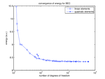
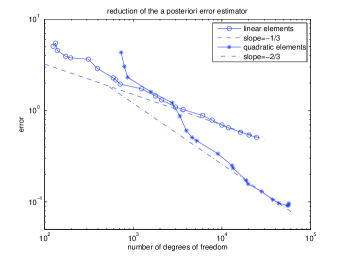
Figure 5.1: Left: Convergence curves of energy for BEC. Right: Reduction of the a posteriori error estimators using linear and quadratic elements.

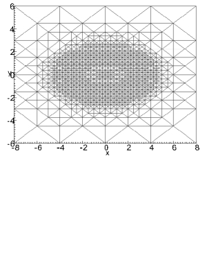
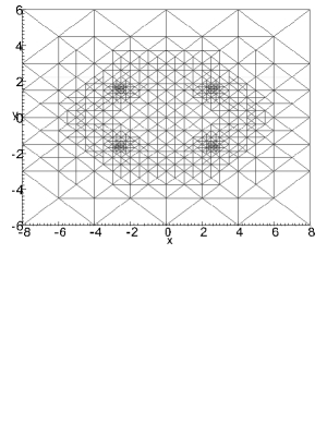
Figure 5.2: The cross-sections on $z=0$ of adaptive meshes using linear (left) and quadratic (right) elements.

In the next two examples, we shall carry out the ground state energy calculations of atomic and molecular systems based on TFW type orbital-free models. The nonlinear term is given by

$$\mathcal{N}(u^{2})=\int_{\mathbb{R}^{3}}\frac{u^{2}(y)}{|\cdot-y|}dy+\frac{5}{3}C_{TF}u^{4/3}+\upsilon_{xc}(u^{2}),$$

where $C_{TF}=\frac{3}{10}(3\pi^{2})^{\frac{2}{3}}$ and $v_{xc}$ is the exchange-correction potential. The exchange-correction potential used in our computation is chosen as

$$\upsilon_{xc}(\rho)=\upsilon_{x}^{LDA}(\rho)+\upsilon_{c}^{LDA}(\rho),$$ (5.2)

where

$$\upsilon_{x}^{LDA}(\rho)=-\left(\frac{3}{\pi}\right)^{1/3}\rho^{1/3},$$

$$\upsilon_{c}^{LDA}(\rho)=\left\{\begin{array}[]{cc}0.0311\ln r_{s}-0.0584+0.0013r_{s}\ln r_{s}-0.0084r_{s}&\mbox{if}~{}r_{s}<1\\[5.69046pt] -(0.1423+0.0633r_{s}+0.1748\sqrt{r_{s}})/(1+1.0529\sqrt{r_{s}}+0.3334r_{s})^{2}&\mbox{if}~{}r_{s}\geq 1\end{array}\right.$$

and $\displaystyle r_{s}=\left(\frac{3}{4\pi\rho}\right)^{1/3}$.

Example 2. Consider the TFW type orbital-free model for helium atoms. The external electrostatic potential is $V(x)=-2/|x|.$ Then we have the following nonlinear problem: Find $(\lambda,u)\in\mathbb{R}\times H^{1}_{0}(\Omega)$ such that $\|u\|^{2}_{0,\Omega}=2$ and

$$\left\{\ \begin{array}[]{rclc}\displaystyle-\frac{1}{10}\Delta u-\frac{2}{|x|}u+u\int_{\Omega}\frac{|u(y)|^{2}}{|x-y|}dy+\frac{5}{3}C_{TF}u^{7/3}+v_{xc}(u^{2})u&=&\lambda u&\mbox{in}~{}\Omega,\\[4.30554pt] u&=&0&\mbox{on}~{}\partial\Omega,\end{array}\right.$$

where $\Omega=(-5.0,5.0)^{3}$.

The convergence of energies and the reduction of the a posteriori error estimators are shown in Figure 5.3, which support our theory. The cross-sections of the adaptive meshes are displayed in Figure 5.4, from which we observe that more refined meshes (nodes) appear in the area where the nuclei are located.

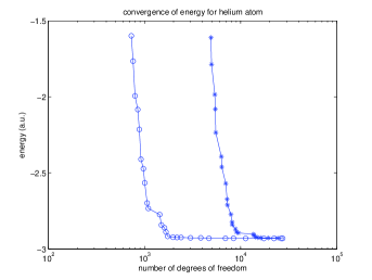
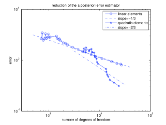
Figure 5.3: Left: Convergence curves of energy for the helium atom. Right: Reduction of the a posteriori error estimators using linear and quadratic elements.

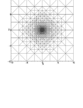
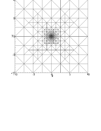
Figure 5.4: The cross-sections on $z=0$ of adaptive meshes using linear (left) and quadratic (right) elements.

Example 3. Finally, we consider an aluminum cluster in the face centered cubic lattice consisting of $3\times 3\times 3$ unit cells with 172 aluminium atoms, where the GHN pseudopotential [26] is used. We solve the following nonlinear problem: Find $(\lambda,u)\in\mathbb{R}\times H^{1}_{0}(\Omega)$ such that $\|u\|^{2}_{0,\Omega}=172$ and

$$\left\{\ \begin{array}[]{rclc}\displaystyle-\frac{1}{10}\Delta u+V_{pseu}^{GHN}u+u\int_{\Omega}\frac{|u(y)|^{2}}{|x-y|}dy+\frac{5}{3}C_{TF}u^{7/3}+v_{xc}(u^{2})u&=&\lambda u&\mbox{in}~{}\Omega,\\[4.30554pt] u&=&0&\mbox{on}~{}\partial\Omega,\end{array}\right.$$

where $\Omega=(-25.0,25.0)^{3}$.

The convergence of energies and the reduction of a posteriori error estimators are shown in Figure 5.5. The cross-sections of the adaptive meshes are displayed in Figure 5.4. We observe that with the a posteriori error estimators, the refinement is carried out automatically at the regions where the computed functions vary rapidly, especially near the nuclei. As a result, the computational accuracy can be controlled efficiently and the computational cost is reduced significantly.

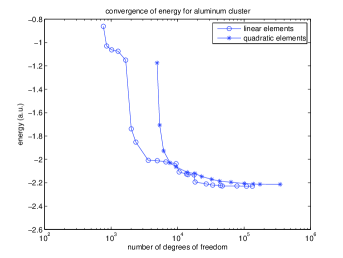
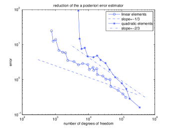
Figure 5.5: Left: Convergence curves of energy for the aluminium cluster in FCC lattice. Right: Reduction of the a posteriori error estimators using linear and quadratic elements.

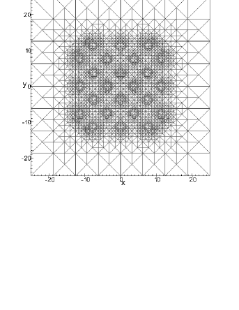
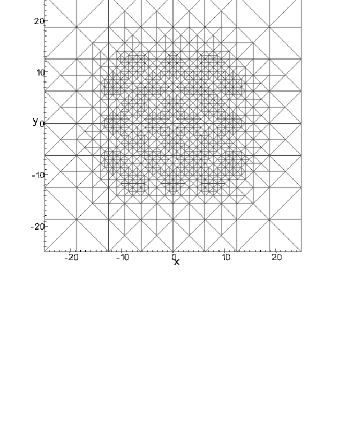
Figure 5.6: The cross-sections on $z=0$ of adaptive meshes using linear and quadratic finite elements.

6 Concluding remarks

We have analyzed adaptive finite element approximations for ground state solutions of a class of nonlinear eigenvalue problems. We have proved that the adaptive finite element loop produces a sequence of approximations that converge to the set of exact ground state solutions. This result covers many mathematical models of practical interest, for instance, the Bose-Einstein condensation, the TFW model in the orbital-free density functional theory, and Schrödinger-Newton equations in the quantum state reduction [15, 27, 35] where the integration kernel $K$ is negative. We have also applied adaptive finite element discretizations to micro-structure of matter calculations, which support our theory. It is shown by Figure 5.1, Figure 5.3, and Figure 5.5 that we may have some convergence rates of adaptive finite element approximations. Indeed, it is our on-going work to study the optimal complexity of adaptive finite element approximations for such nonlinear eigenvalue problems, which requires a new technical tool and will be addressed elsewhere [16].

Acknowledgements. The authors would like to thank Dr. Xiaoying Dai, Prof. Lihua Shen, and Dr. Dier Zhang for their stimulating discussions and fruitful cooperations on electronic structure computations that have motivated this work. The authors are grateful to Prof. Linbo Zhang and Mr. Hui Liu for their assistance on numerical computations.

Appendix

We may follow the framework in [39] to derive an upper bound and a lower bound of the a posteriori error estimate. Let

$$X~{}=~{}Y~{}=~{}H_{0}^{1}(\Omega),$$

$$\|\cdot\|_{X}~{}=~{}\|\cdot\|_{Y}~{}=~{}\|\cdot\|_{1,\Omega},$$

$$\langle F(\lambda,u),(\mu,v)\rangle=\int_{\Omega}\big{(}\alpha\nabla u\nabla v+Vuv+\mathcal{N}(u^{2})uv-\lambda uv\big{)}+\mu\big{(}\int_{\Omega}u^{2}-Z\big{)}.$$

It is seen that (2.3) may be written as

$$F(\lambda,u)=0$$ (A.1)

and $F\in C^{1}(\mathbb{R}\times X,\mathbb{R}\times Y^{*})$, where $Y^{*}$ is the dual space of $Y$. A solution $(\lambda,u)$ of (A.1) is said to be regular if the following equation

$$DF(\lambda,u)\cdot(\mu,v)=(\kappa,f)$$

is uniquely solvable in $\mathbb{R}\times X$ for each $(\kappa,f)\in\mathbb{R}\times Y^{*}$, where $DF(\lambda,u):~{}\mathbb{R}\times X\rightarrow\mathbb{R}\times Y^{*}$ is the Fréchet derivative of $F$ at $(\lambda,u)$. It is seen that $(\lambda,u)\in\mathbb{R}\times H^{1}_{0}(\Omega)$ is a regular solution of (A.1) if

$$\langle(E^{\prime\prime}(u)-\lambda)v,v\rangle_{Y^{*},X}\geq\gamma\|\nabla v\|^{2}_{0,\Omega}\quad\forall~{}v\in H_{0}^{1}(\Omega)\cap u^{\bot}$$ (A.2)

is true for some constant $\gamma>0$ (see, e.g., [29]), where

$$\langle(E^{\prime\prime}(u)-\lambda)v,w\rangle = \alpha(\nabla v,\nabla w)+((V+\mathcal{N}(u^{2})-\lambda)v,w)+2(\mathcal{N}_{1}^{\prime}(u^{2})u^{2}v,w)$$

$$+2qD_{K}(u^{2q-1}v,u^{2q-1}w)+2(q-1)(\mathcal{N}_{2}(u^{2})v,w)$$

and

$$u^{\bot}=\{w\in L^{2}(\Omega):(u,w)=0\}.$$

It has been proved that (A.2) is satisfied by some special TFW models that are of convex functional (see, e.g., [10, 11]).

Let

$$X_{h}~{}=~{}Y_{h}~{}=~{}S_{0}^{h}(\Omega)~{}$$

and define

$$\langle F_{h}(\lambda_{h},u_{h}),(\mu,v)\rangle~{}=~{}\langle F(\lambda_{h},u_{h}),(\mu,v)\rangle\quad\forall~{}(\mu,v)\in\mathbb{R}\times S_{0}^{h}(\Omega).$$

We see that $F_{h}\in C(\mathbb{R}\times X_{h},\mathbb{R}\times Y_{h}^{*})$ and is an approximation of $F$. Obviously, finite element eigenvalue problem (3.16) is equivalent to

$$F_{h}(\lambda_{h},u_{h})=0$$

and $(\lambda_{h},u_{h})$ is an approximate solution of (A.1).

The following proposition in [39, Section 2.1] yields a posteriori error estimates in the neighborhood of $(\lambda,u)$ that satisfies (A.1).

Proposition A.1.

Let $(\lambda,u)$ be a regular solution of (A.1). If $DF$ is the derivative of $F$ and $DF$ is Lipschitz continuous at $(\lambda,u)$, then the following estimate holds for all $(\lambda_{h},u_{h})$ sufficiently close to this solution:

$$\|F(\lambda_{h},u_{h})\|_{\mathbb{R}\times Y^{*}}\lesssim|\lambda_{h}-\lambda|+\|u_{h}-u\|_{X}\lesssim\|F(\lambda_{h},u_{h})\|_{\mathbb{R}\times Y^{*}}.$$ (A.3)

It is shown from (A.3) that $\|F(\lambda_{h},u_{h})\|_{\mathbb{R}\times Y^{*}}$ is a posteriori error estimator. When we apply the general approach in [39, Sections 3.3-3.4] to

$$\underline{a}(x,u,\nabla u)=\alpha\nabla u\quad\mbox{and}\quad b(x,u,\nabla u)=\lambda u-Vu-\mathcal{N}(u^{2})u$$

by taking

$$\underline{a}_{h}(x,u_{h},\nabla u_{h})=\alpha\nabla u_{h},\quad b_{h}(x,u_{h},\nabla u_{h})=\overline{\lambda u_{h}}-\overline{Vu_{h}}-\overline{\mathcal{N}(u_{h}^{2})u_{h}},$$

and

$$\eta_{T}=\eta_{h}(u_{h},T),\quad\varepsilon_{T}={\rm osc}_{h}(u_{h},T),$$

we then gives a proof of Theorem 3.1.