Quantum dynamics in the bosonic Josephson junction

Abstract

We employ a semiclassical picture to study dynamics in a bosonic Josephson junction with various initial conditions. Phase-diffusion of coherent preparations in the Josephson regime is shown to depend on the initial relative phase between the two condensates. For initially incoherent condensates, we find a universal value for the buildup of coherence in the Josephson regime. In addition, we contrast two seemingly similar on-separatrix coherent preparations, finding striking differences in their convergence to classicality as the number of particles increases.

I Introduction

Bose-Einstein condensates (BECs) of dilute, weakly-interacting gases offer a unique opportunity for exploring non-equilibrium many-body dynamics, far beyond small perturbations of the ground state. Highly excited states are naturally produced in BEC experiments and their dynamics can be traced with great precision and control. The most interesting possibilities lie in strong correlation effects, which imply a significant role of quantum fluctuations.

The importance of correlations and fluctuations may be enhanced by introducing an optical lattice, that can be controlled by tuning its depth. This tight confinement decreases the kinetic energy contribution with respect to the interactions between atoms. In the tight-binding limit, such systems are described by a Bose-Hubbard Hamiltonian (BHH), characterized by the hopping frequency $K$ between adjacent lattice sites, the on-site interaction strength $U$, and the total atom number $N$. The strong correlation regime is attained when the characteristic coupling parameter $u\equiv UN/K$ exceeds unity, as indicated by the quantum phase transition from a superfluid to a Mott-insulator Jaksch98 ; Greiner02a .

The simplest BHH is obtained for two weakly coupled condensates (dimer). Its dynamics is readily mapped onto a SU(2) spin problem and is closely related to the physics of superconductor Josephson junctions BJM ; Leggett01 . To the lowest order approximation, it may be described by a Gross-Pitaevskii mean-field theory, accurately accounting for Josephson oscillations Javanainen86 ; Dalfovo96 ; Zapata98 and macroscopic self trapping Smerzi97 , observed experimentally in Refs.Cataliotti01 ; Albiez05 , as well as the equivalents of the ac and dc Josephson effect Giovanazzi00 observed in Levy07 .

Both Josephson oscillations and macroscopic self trapping rely on coherent (Gaussian) preparations, with different initial population imbalance. The mean-field premise is that such states remain Gaussian throughout their evolution so that the relative phase $\varphi$ between the two condensates remains defined. However, interactions between atoms lead to the collapse and revival of the relative phase in a process known as phase diffusion Leggett98 ; Wright96 ; Javanainen97 . (the appropriate term is in fact phase spreading). Phase diffusion has been observed with astounding precision in an optical lattice in Refs.Greiner02 , in a double-BEC system in Refs.Jo07 ; Schumm05 ; Hofferberth07 , and in a 1D spinor BEC in Ref. Widera08 . Typically, the condensates are coherently prepared, held for a varying duration (‘hold time’) in which phase-diffusion takes place, and are then released and allowed to interfere, thus measuring the relative coherence through the many-realization fringe visibility. In order to establish this quantity, the experiment is repeated many times for each hold period.

Phase-diffusion experiments focus on the initial preparation of a zero relative phase and its dispersion when no coupling is present between the condensates. However, in the presence of weak coupling during the hold time, the dynamics of phase diffusion is richer. It becomes sensitive to initial value of $\varphi$ and the loss of coherence is most rapid for $\varphi=\pi$ Vardi01 ; Khodorkovsky08 ; Boukobza09 . Here, we expand on a recent letter Boukobza09 , showing that this quantum effect can be described to excellent accuracy by means of a semiclassical phase-space picture. Furthermore, exploiting the simplicity of the dimer phase space, we derive analytical expressions based on the classical phase-space propagation SmithMannschott09 .

Phase-space methods GardinerZoller have been extensively applied for the numerical simulation of quantum and thermal fluctuation effects in BECs Steel98 ; Sinatra01 ; Carusotto01 ; Hoffmann08 ; Polkovnikov03 ; Plimak03 ; Deuar06 ; Isella06 ; HKG06 ; Midgley09 ; Deuar09 ; Trimborn08 ; Mahmud . Such methods utilize the semiclassical propagation of phase-space distributions with quantum fluctuations emulated via stochastic noise terms, and using a cloud of initial conditions that reflects the uncertainty of the initial quantum wave-packet. One particular example is the truncated Wigner approximation Sinatra01 ; Polkovnikov03 ; Isella06 ; Midgley09 where higher order derivatives in the equation of motion for the Wigner distribution function are neglected, thus amounting to the propagation of an ensemble using the Gross-Pitaevskii equations.

Due to the relative simplicity of the classical phase-space of the two-site BHH, it is possible to carry out its semiclassical quantization semi-analytically Boukobza09 ; SmithMannschott09 ; Boukobza09a ; Franzosi00 ; Graefe07 and acquire great insight on the ensuing dynamics of the corresponding Wigner distribution wignerfunc ; Agarwal81 . In this work, we consider the Jopheson-regime dynamics of four different preparations, interpreting the results in terms of the semiclassical phase-space structure and its implications on the expansion of each of these initial states in terms of the semiclassical eigenstates. We first explore the phase-sensitivity of phase-diffusion in the Josephson regime Vardi01 ; Boukobza09 . Then we study the buildup of coherence between two initially separated condensates Boukobza09a , which is somewhat related to the phase-coherence oscillations observed in the sudden transition from the Mott insulator to the superfluid regime in optical lattices Polkovnikov02 ; Altman02 ; Tuchman06 . Then we compare two coherent preparations in the separatrix region of the classical phase space, finding substantial differences in their dynamics due to their different participation numbers.

The narrative of this work is as follows a : The two-site Bose-Hubbard model and its classical phase-space are presented in Section II. The semiclassical WKB quantization is carried out in Section III. In Section IV, we define the initial state preparations of interest and explain their phase-space representation. This is used in Section V to evaluate their expansion in the energy basis (the local density of states), which is the key for studying the dynamics in Sections VI to VIII. Both the time-averaged dynamics and the fluctuations of the Bloch vector are analyzed. In particular we observe in Section VIII that the fluctuations obeys a remarkable semiclassical scaling relation. Conclusions are given in Section X.

II The two-site Bose-Hubbard model

We consider the Bose-Hubbard Hamiltonian for $N$ bosons in a two-site system,

$$\mathcal{H}\ =\ \sum_{i=1,2}\left[\mathcal{E}_{i}\bm{n}_{i}+\frac{U}{2}\bm{n}_{i}(\bm{n}_{i}-1)\right]-\frac{K}{2}(\hat{a}_{2}^{{\dagger}}\hat{a}_{1}+\hat{a}_{1}^{{\dagger}}\hat{a}_{2}),$$ (1)

where $K$ is the hopping amplitude, $U$ is the interaction, and ${\mathcal{E}=\mathcal{E}_{2}-\mathcal{E}_{1}}$ is the bias in the on-site potentials. We use boldface fonts to mark dynamical variables that are important for the semiclassical analysis, and use regular fonts for their values. The total number of particles ${n_{1}+n_{2}=N}$ is conserved, hence the dimension of the pertinent Hilbert space is ${\mathcal{N}=N+1}$. Defining

$${{J}}_{z}\ \ \equiv \ \ \frac{1}{2}(\bm{n}_{1}-\bm{n}_{2})\ \ \equiv\ \ \bm{n},$$ (2)

$${{J}}_{+}\ \ \equiv \ \ \hat{a}_{1}^{{\dagger}}\hat{a}_{2}$$ (3)

and eliminating insignificant $c$-number terms, we can re-write Eq. (1) as a spin Hamiltonian,

$$\mathcal{H}\ =\ U{{J}}_{z}^{2}-\mathcal{E}{{J}}_{z}-K{{J}}_{x},$$ (4)

conserving the spin $J^{2}=j(j+1)$ with $j=N/2$. The BHH Hamiltonian thus has a spherical phase-space structure. In the absence of interaction ($U=0$) it describes simple spin precession with frequency ${\Omega=(K,0,\mathcal{E})}$.

The quantum evolution of the spin Hamiltonian (4) is given by the unitary operator $\exp(-i\mathcal{H}t)$. Its classical limit is obtained by treating ${(J_{x},J_{y},J_{z})}$ as $c$-numbers, whose Poisson Brackets (PB) correspond to the SU(2) Lie algebra. The classical equations of motion for any dynamical variable $A$ are derived from ${\dot{A}=-[\mathcal{H},A]_{\mbox{\tiny PB}}}$. Conservation of $J^{2}$ allows for one constraint on the non-canonical set of variables ${(J_{x},J_{y},J_{z})}$.

Due to the spherical phase-space geometry, it is natural to use the non-canonical conjugate variables ${(\bm{\varphi},\bm{\theta})}$,

$${{J}}_{z} \equiv [{{J}}^{2}]^{1/2}\cos(\bm{\theta})$$ (5)

$${{J}}_{x} \equiv [{{J}}^{2}]^{1/2}\sin(\bm{\theta})\cos(\bm{\varphi})$$ (6)

where $[{{J}}^{2}]^{1/2}$ is a constant of the motion. In the quantum mechanical Wigner picture treatment (see later sections) this constant is identified as $[(j{+}1)j]^{1/2}$, based on the derivation of section 2.3 of Ref. wignerfunc . For large $j$ we use ${[{{J}}^{2}]^{1/2}\approx N/2}$. With these new variables the Hamiltonian takes the form

$$H(\bm{\theta},\bm{\varphi})=\frac{NK}{2}\left[\frac{1}{2}u(\cos\bm{\theta})^{2}-\varepsilon\cos\bm{\theta}-\sin\bm{\theta}\cos\bm{\varphi}\right],$$ (7)

where the scaled parameters are

$$u\equiv\displaystyle{\frac{NU}{K}},\hskip 56.9055pt\varepsilon\equiv\displaystyle{\frac{\mathcal{E}}{K}}.$$ (8)

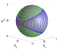
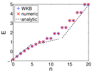
Figure 1: (Color online) Contour lines for $u>2$. Sea levels are colored blue, Island levels are colored green, and the Separatrix is colored red (left panel). Energy spectrum for $N={20}$ and $u=10$. WKB energies (red x) are compared with exact eigenvalues (blue +). Dashed lines indicate slopes $\omega_{J}$ for low energies, $\omega_{x}$ for near-separatrix energies, and $\omega_{+}$ for high energies (right panel).

The structure of the underlying classical phase space is determined by the dimensionless parameters $u$ and $\varepsilon$. For strong interactions ${u>1}$ the phase space includes a figure-eight shaped separatrix (Fig. 1), provided $\left|\varepsilon\right|<\varepsilon_{c}$, where WN00 ; SmithMannschott09

$$\varepsilon_{c}=\left(u^{\frac{2}{3}}-1\right)^{\frac{3}{2}}.$$ (9)

This separatrix splits phase space into three integrable regions: a ‘sea’ of Rabi-like trajectories and two interaction-dominated nonlinear ‘islands’. For zero bias the separatrix is a symmetric $8$ shaped figure that encloses the two islands, and the relevant energies are ELS85

$$E_{-}= -(1/2)NK =\mbox{ground energy},$$ (10)

$$E_{\mbox{\tiny x}}= +(1/2)NK =\mbox{separatrix},$$ (11)

$$E_{+}= (1/4)[u{+}(1/u)]NK =\mbox{top energy}.$$ (12)

Looking at the phase-space structure as a function of $u$, the two islands emerge once ${u>1}$. For ${u>2}$, they encompass the North and the South poles, yielding macroscopic self-trapping Smerzi97 , and for very large ${u\gg 1}$ they cover most of the Northern and the Southern hemispheres respectively. Note that for $u\gg 1$, the expression ${E_{+}\approx(N/2)^{2}U}$, reflects the cost of localizing all the particles in one site, compared to equally-populated sites.

As an alternative to Eq. (7), it is possible to employ the relative number-phase representation, using the canonically conjugate variables ${(\bm{\varphi},\bm{n})}$, with the Hamiltonian,

$$\mathcal{H}\ \ =\ \ U\bm{n}^{2}\ -\ \mathcal{E}\bm{n}\ -\ K\sqrt{(N/2)^{2}-\bm{n}^{2}}\ \cos(\bm{\varphi}).$$ (13)

In the ${|n|\ll(N/2)}$ region of phase space, one obtains the Josephson Hamiltonian, which is essentially the Hamiltonian of a pendulum

$$\mathcal{H}_{\mbox{\tiny Josephson}}\ \ =\ \ E_{C}(\bm{n}-n_{\varepsilon})^{2}\ -\ E_{J}\cos(\bm{\varphi})$$ (14)

with $E_{C}=U$ and $E_{J}=KN/2$ while $n_{\varepsilon}$ is linearly related to $\mathcal{E}$. The Josephson Hamiltonian ignores the spherical geometry, and regards phase space as cylindrical. Accordingly it captures much of the physics if the motion is restricted to the small-imbalance slice of phase-space, as in the case of equal initial populations and strong interactions. However, for other regimes it is an over-simplification because it does not correctly capture the global topology.

III The WKB quantization

We begin by stipulating the procedure for the semiclassical quantization of the spin spherical phase-space. In the ${(\varphi,n)}$ representation, the area element is ${d\Omega=d\varphi dn}$, so that the total phase-space area is $2\pi N$ with Planck cell ${h=2\pi}$. Alternatively, using the ${(\varphi,\theta)}$ coordinates, the area element is ${d\Omega=d\varphi d\cos\theta}$, so that the total area is $4\pi$. Consequently

$$h\ =\ \mbox{Planck cell area in steradians}\ =\ \frac{4\pi}{\mathcal{N}}.$$ (15)

Within the framework of the semiclassical picture, eigenstates are associated with stripes of area $h$ that are stretched along contour lines ${\mathcal{H}(\varphi,\theta)=E}$ of the classical Hamiltonian $\mathcal{H}$. The associated WKB quantization condition is

$$A(E_{\nu})=\left(\frac{1}{2}+\nu\right)h,\ \ \ \ \ \ \nu=0,1,2,...$$ (16)

where $A(E)$ is defined as the phase-space area enclosed by an $E$ contour in steradians:

$$A(E)\ \ \equiv\ \ \iint\Theta(E-\mathcal{H}(\varphi,\theta))\ d\Omega,$$ (17)

while the area of phase space in Planck units is $A(E)/h$. The frequency of oscillations at energy $E$ is

$$\omega(E)\ \ \equiv\ \ \frac{dE}{d\nu}\ \ =\ \ \left[\frac{1}{h}A^{\prime}(E)\right]^{-1}.$$ (18)

Consider the semiclassical quantization of the Hamiltonian (7). We distinguish three regimes of interaction strength. Assuming ${\varepsilon=0}$, these are

Rabi regime: $$u<1$$ (no islands) (19)

Josephson regime: $$1<u<N^{2}$$ (see Fig. 1) (20)

Fock regime: $$u>N^{2}$$ (empty sea) (21)

In the Fock regime, the area of the sea becomes less than a single Planck cell, and therefore cannot support any eigenstates. Our interest throughout this paper is mainly in the Josephson regime where neither the $K$ term nor the $U$ term can be regarded as a small perturbation in the Hamiltonian. This regime, characteristic of current atom-interferometry experiments, is where semiclassical methods become most valuable.

In the WKB framework the spacing between energies equals the characteristic classical frequency at this energy. If the interaction is zero ($u=0$), the energy levels are equally spaced and there is only one frequency, namely the Rabi frequency

$$\omega_{K}\ \ =\ \ K$$ (22)

For small interaction (${0<u<1}$) the frequencies around the two stable fixed points are slightly modified to the plasma frequencies:

$$\omega_{\pm}\ \ =\ \ \omega(E_{\pm})\ \ =\ \ \sqrt{(K\pm NU)K}.$$ (23)

If the interaction is strong enough ($u\gg 1$), the oscillation frequency near the minimum point can be approximated as

$$\omega_{J}\ \ =\ \ \omega(E_{-})\ \ \approx\ \ \sqrt{NUK}\ \ =\ \ \sqrt{u}\ \omega_{K},$$ (24)

while at the top of the islands we have:

$$\omega_{+}\ \ =\ \ \omega(E_{+})\ \ \approx\ \ NU\ \ =\ \ u\ \omega_{K}.$$ (25)

The associated approximations for the phase-space area in the three energy regions (bottom of the sea, separatrix, and top of the islands) are respectively

$$\frac{1}{h}A(E) = \left(\frac{E-E_{-}}{\omega_{J}}\right),$$ (26)

$$\frac{1}{h}A(E) = \frac{1}{h}A(E_{\mbox{\tiny x}})+\frac{1}{\pi}\left(\frac{E-E_{\mbox{\tiny x}}}{\omega_{J}}\right)\log\left|\frac{NK}{E-E_{x}}\right|,$$ (27)

$$\frac{1}{h}A(E) = \frac{4\pi}{h}-\left(\frac{E_{+}-E}{U}\right)^{1/2},$$ (28)

In the last expression the total area of the two islands ${(E_{+}{-}E)/U}$ should be divided by two if one wants to obtain the area of a single island. A few words are in order regarding the derivation of Eq. (27). In the vicinity of the unstable fixed point the contour lines of the Hamiltonian are ${Un^{2}-(NK/4)\varphi^{2}=E{-}E_{\mbox{\tiny x}}}$, where for convenience the origin is shifted ($\varphi{=}\pi\mapsto 0$). Defining $a^{2}=4(E{-}E_{\mbox{\tiny x}})/NK$ the area of the region above the separatrix is $2(NK/4U)^{1/2}[\mathcal{A}(a)-\mathcal{A}(0)]$ where $\mathcal{A}(a)$ is the integral over $\sqrt{\varphi^{2}+a^{2}}$. The result of the integration is ${\mathcal{A}(a)-\mathcal{A}(0)=a^{2}\log(b/a)}$, with some ambiguity with regard to $b\sim 1$ which is determined by the outer limits of the integral where the hyperbolic approximation is no longer valid.

Away from the separatrix, the WKB quantization recipe implies that the local level spacing at energy $E$ is $\omega(E)$ given by Eq. (18). In particular, the low energy levels have spacing $\omega_{J}$, while the high energy levels are doubly-degenerate with spacing $\omega_{+}$. In the vicinity of the separatrix we get

$$\omega(E)\ \ \approx\ \ \left[\frac{1}{\pi}\log\left|\frac{NK}{E-E_{x}}\right|\right]^{-1}\omega_{J}.$$ (29)

Using the WKB quantization condition, we find that the level spacing at the vicinity of the separatrix ($E\sim E_{\mbox{\tiny x}}$) is finite and given by the expression

$$\omega_{\mbox{\tiny x}}\ \ =\ \ \left[\log\left(N/\sqrt{u}\right)\right]^{-1}\omega_{J}.$$ (30)

Using an iterative procedure one finds that at the same level of approximation the near-separatrix energy levels are

$$E_{\nu}=E_{\mbox{\tiny x}}+\left[\frac{1}{\pi}\log\left|\frac{N/\sqrt{u}}{\nu{-}\nu_{\mbox{\tiny x}}}\right|\right]^{-1}(\nu{-}\nu_{\mbox{\tiny x}})\ \omega_{J},$$ (31)

where $\nu_{\mbox{\tiny x}}=A(E_{\mbox{\tiny x}})/h$. Fig. 1 demonstrates the accuracy of the WKB quantization, and of the above approximations.

IV The initial preparation and its phase-space representation - the Wigner function

Our approach for investigating the dynamics of various initial preparations relies on the Wigner-function formalism for spin variables, developed in Refs. Agarwal81 ; wignerfunc . Each initial preparation is described as a Wigner distribution function over the spherical phase space. The dynamics is deduced from expanding the initial state in terms of the semiclassical eigenstates described in Sec III. In this section we specify the Wigner distribution for the preparations under study whereas the following section presents the eigenstate expansion of each of these four initial wavepackets, evaluated semiclassically.

To recap the phase-space approach to spin Agarwal81 ; wignerfunc , the Hilbert space of the BHH has the dimension $\mathcal{N}=2j{+}1$, and the associated space of operators has the dimensionality $\mathcal{N}^{2}$. According to the Stratonovich-Wigner-Weyl correspondence (SWWC) Stratonovich56 , any observable $A$ in this space, as well as the probability matrix of a spin^(j) entity, can be represented by a real sphere^(2j) function $A_{\mbox{\tiny W}}(\Omega)$. The sphere^(2j) is spanned by the $Y^{\ell m}(\Omega)$ functions with ${\ell\leq 2j}$, and the practical details regarding this formalism can be found in Refs. Agarwal81 ; wignerfunc . The SWWC allows to do exact quantum calculation in a classical-like manner. A few examples for Wigner functions pertinent to this work, are displayed in Fig. 2. Expectation values are calculated as in classical statistical mechanics:

$$\text{trace}[\hat{\rho}\ \hat{A}]\ \ =\ \ \int\frac{d\Omega}{h}{\rho_{\mbox{\tiny W}}(\Omega)A_{\mbox{\tiny W}}(\Omega)}$$ (32)

In particular the Wigner-Weyl representation of the identity operator is $1$, and that of $J_{x}$ is as expected $[(j{+}1)j]^{1/2}\sin(\theta)\cos(\varphi)$ wignerfunc . We adopt the convention that $\rho_{\mbox{\tiny W}}$ is normalized with respect to the measure $d\Omega/h$, allowing to handle on equal footing a cylindrical phase space upon the re-identification ${d\Omega=d\varphi dn}$ and ${h=2\pi}$.

Within this phase-space representation, the Fock states $|n\rangle$ are represented by stripes along constant $\theta$ contours (see e.g. left panel of Fig. 2). The ${|n{=}N\rangle}$ state (all particles in one site) is a Gaussian-like wave packet concentrated around the NorthPole. From this state, we can obtain a family of spin coherent states (SCS) ${|\theta,\varphi\rangle}$ via rotation.

In what follows, we explore the dynamics of the following experimentally-accessible preparations (see Fig. 2), the first being a Fock state, whereas the last three are spin coherent states:

• TwinFock preparation: The $n{=}0$ Fock preparation. Exactly half of the particles are in each side of the double well. The Wigner function is concentrated along the equator $\theta=\pi/2$.

• Zero preparation: Coherent $(\theta{=}\pi/2,\varphi{=}0)$ preparation, located entirely in the (linear) sea region. Both sites are equally populated with definite $0$ relative phase. The minimal wave-packet is centered at $(n=0,\varphi=0)$.

• Pi preparation: Coherent $(\theta{=}\pi/2,\varphi{=}\pi)$ on-separatrix preparation. The sites are equally populated with $\pi$ relative phase. The minimal wave-packet is centered at $(n=0,\varphi=\pi)$.

• Edge preparation: Coherent $\varphi\neq\pi$ on-separatrix preparation. The minimal wave-packet is centered on the separatrix but away from the saddle point on the $\varphi{=}0$ side.

The Wigner function of an SCS resembles a minimal Gaussian wave-packet, and it should satisfy

$$\int\rho_{\mbox{\tiny W}}(\theta,\varphi)\frac{d\Omega}{h}=\int[\rho_{\mbox{\tiny W}}(\theta,\varphi)]^{2}\frac{d\Omega}{h}=1.$$ (33)

This requirement helps to determine the phase space spread without the need to use the lengthy algebra of Refs. Agarwal81 ; wignerfunc . For the Fock coherent state ${|n{=}N\rangle}$, that is centered at the NorthPole ($\theta=0$), one obtains:

$$\rho_{\mbox{\tiny W}}^{(\psi)}(\theta,\varphi)\approx 2\mbox{e}^{-\frac{\mathcal{N}}{2}\theta^{2}}~{}.$$ (34)

For the coherent states centered around the Equator, it is more convenient to use ${(\varphi,n)}$ coordinates, e.g. the $\varphi=0$ coherent state is well approximated as,

$$\rho_{\mbox{\tiny W}}^{(\psi)}(n,\varphi)\ \ \approx\ \ \frac{1}{ab}\mbox{e}^{-\frac{\varphi^{2}}{2a^{2}}-\frac{n^{2}}{2b^{2}}}~{},$$ (35)

with $a=1/\sqrt{2\mathcal{N}}$ and $b=\sqrt{\mathcal{N}/2}$. Shifted versions of these expressions describe the ${\varphi=\pi}$ and the “Edge” preparations. The Wigner function of a Fock state ${\psi=|\mathsf{n}\rangle}$ is semiclassically approximated as

$$\rho_{\mbox{\tiny W}}^{(\psi)}(n,\varphi)\ \ \approx\ \ \delta(n-\mathsf{n}),$$ (36)

whereas the Wigner function of an eigenstate is semiclassically approximated by a micro-canonical distribution:

$$\rho_{\mbox{\tiny W}}^{(\nu)}(n,\varphi)\ \ \approx\ \ \omega(E_{\nu})\ \delta(\mathcal{H}(\varphi,n)-E_{\nu}).$$ (37)

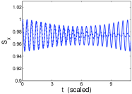
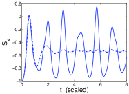
(c)                                (d)                               

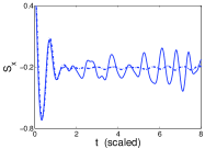
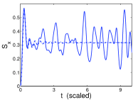
Figure 4: (Color online) The variation of $S_{x}(t)$ with time for $N{=}40$ particles with $u=5$, for Zero (a), Pi (b), Edge (c), and TwinFock (d) preparations. Note the different vertical scale. The dashed-dotted lines are based on semiclassical simulation. Note that the fluctuations of a semiclassical preparation always die after a transient, which should be contrasted with both the classical (single trajectory) and quantum (superposition of ${M>1}$ eigenstates) behavior.

In general none of the above listed initial states is an eigenstate of the BHH, but rather a superposition of BHH eigenstates. Consequently their Wigner function deforms over time (see e.g. Fig. 3) and the expectation values of observables become time dependent (see e.g.Fig. 4), as discussed in later sections.

V The initial preparation and its eigenstate expansion - local density of states

Having set the stage by defining the phase-space representation of eigenstates in Sect. III and of the initial conditions in Sect. IV, the evolution of any initial preparation is uniquely determined by its eigenstate expansion. Thus, in order to analyze the dynamics, we now evaluate the local density of states (LDOS) with respect to the preparation $\psi$ of the system:

$$\mbox{P}(E_{\nu}) = |\langle E_{\nu}|\psi\rangle|^{2}=\mbox{trace}(\rho^{(\nu)}\rho^{(\psi)})$$ (38)

$$= \int\rho_{\mbox{\tiny W}}^{(\nu)}(\Omega)\ \rho_{\mbox{\tiny W}}^{(\psi)}(\Omega)\frac{d\Omega}{h}.$$

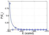
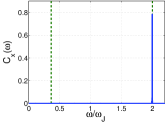
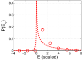
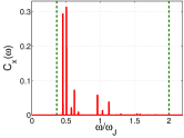
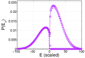
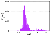
Figure 5: (Color online) The LDOS (left) and the spectral content of the fluctuations (right) of $N=500$ bosons with $u=4$, for Zero, Pi, Edge, and TwinFock preparations (top to bottom). The horizontal axes are $E-E_{\mbox{\tiny x}}$ and $\omega/\omega_{J}$. The lines in the LDOS figures are based on a semiclassical analysis (see text), while the circles are from the exact quantum calculation. Note that due to the mirror symmetry of the Zero preparation the expected frequency should approach $2\omega_{J}$, while for the Pi preparation it is bounded from below by $2\omega_{\mbox{\tiny x}}$ (both frequencies are indicted by vertical dashed lines). Note also the outstanding difference between the spectral support of Zero and Pi preparations compared with continuous-like support in the case of Edge and Fock preparations.

If $\psi$ is mirror symmetric the above expression should be multiplied either by 0 or by 2 in the case of odd/even eigenstates. In Fig. 5, we plot the LDOS associated with Pi, Edge, Zero and TwinFock preparations. The applicability of semiclassical methods to calculate the LDOS has been numerically demonstrated for the case of a three site (trimer) model in HKG06 . By contrast, the simpler two site (dimer) model under consideration, offers an opportunity for deriving exact expressions by substituting Eqs. (35)-(37) into Eq. (38) and evaluating the integrals under the appropriate approximations. For clarity, we summarize below the main results of this analytic evaluation, with the details given in App. D.

Consider first the Pi and Edge preparations. The Wigner distributions of both lie on the separatrix and are hence concentrated around the energy $E_{\mbox{\tiny x}}$. Yet, their line shapes are strikingly different: For an Edge preparation we have,

$$\mbox{P}(E)\ \propto\ \frac{\omega(E)}{\omega_{J}}\ \exp\left[-\frac{1}{\mathcal{N}}\left(\frac{E-E_{\mbox{\tiny x}}}{\omega_{J}}\right)^{2}\right]~{},$$ (39)

featuring a dip at $E\sim E_{\mbox{\tiny x}}$. The calculation in the Pi case leads to

$$\mbox{P}(E)\ \propto\ \frac{\omega(E)}{\omega_{J}}\ \mbox{Bessel}\left[\frac{E-E_{\mbox{\tiny x}}}{NU}\right]$$ (40)

(the exact expression can be found in App. D). This latter line shape features a peak at $E\sim E_{\mbox{\tiny x}}$, because the Bessel function compensates the logarithmic suppression by $\omega(E)$. Consequently, as seen below, the fluctuations associated with on-separatrix motion differ dramatically, depending on where the SCS wave-packet is launched.

Analytic results are obtained in App. D, also for the Zero and TwinFock preparations. In the latter case the result is:

$$\mbox{P}(E)\ \propto\ \frac{\omega(E)}{NK}\left[1-\left(\frac{2E}{NK}\right)^{2}\right]^{-1/2}~{}.$$ (41)

As shown in Fig. 5, the above semiclassical expressions agree well with the exact numerical results.

The LDOS determines the spectral content of the dynamics. Consider first the characteristic oscillation frequency of dynamical variables. Away from the separatrix, it is given by the classical estimate $\omega_{\mbox{\tiny osc}}\approx\omega(E)$. For example, for a Zero preparation, we have ${\omega_{\mbox{\tiny osc}}=\omega_{J}}$. While the classical frequency vanishes on the separtrix, we still obtain a finite result for near-separatrix preparations (Pi,Edge) because the wave-packet has a finite width, and because $\omega_{\mbox{\tiny x}}$ provides a lower bound on $\omega_{\mbox{\tiny osc}}$. In any case the result becomes $h$ dependent. To be specific, consider the Pi and the Edge preparations separately. In both cases the width of the wave-packet is $\Delta n=\sqrt{N/2}$. In case of the Pi preparation it occupies an energy range ${\Delta E=U\Delta n^{2}\propto N}$, while in the Edge preparation case ${\Delta E=v_{n}\Delta n\propto N^{1/2}}$, where $v_{n}\approx\omega_{J}$ is identified as the velocity of the phase space points in this region. Using Eq. (29) we find

$$\omega_{\mbox{\tiny osc}}\approx\left\{\begin{matrix}1\cr 2\end{matrix}\right\}\times\left[\log\left(\frac{N}{u}\right)\right]^{-1}\omega_{J},$$ (42)

where the additional factor of “2” applies to the Edge preparation: This factor is due to the different dependence of $\Delta E$ on $N$ in the two respective cases. On top we might have an additional factor of $2$ due to mirror symmetry (see discussion of the dynamics at the end of the next section). Note that as $u/N$ exceeds unity, the distinction between Pi, Zero, and Edge preparations blurs because the wave-packets becomes wider than the width of the separatrix region, until at the Fock regime, all three consist of the same island levels. Thus in this limit, we get for $\omega_{\mbox{\tiny osc}}$ essentially the same result as in the (negligable $K$) Fock regime: the width of the wave-packet is $\Delta n=\sqrt{N/2}$, and the dispersion relation $\omega(E)=2Un$ gives the standard separated-condensates phase-diffusion frequency Greiner02 ; Jo07 ,

$$\omega_{\mbox{\tiny osc}}\ \approx\ \left(\frac{u}{N}\right)^{1/2}\omega_{J}\ =\ U\sqrt{N}.$$ (43)

It should be clear that, both, in Eq. (42) and in Eq. (43) $u/N$ should be accompanied with a numerical prefactor that should be adjusted because the notion of “width” is somewhat ill defined and in general depends on the precise details of the numerical procedure, which we discuss in the next section.

For the analysis of the temporal fluctuations it is crucial to determine the number of eigenstates that participate in the wave-packet superposition. This is given by the LDOS participation number,

$$M\ \ =\ \ \left[\sum_{\nu}\mbox{P}(E_{\nu})^{2}\right]^{-1}.$$ (44)

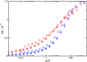
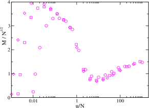
Figure 6: (Color online) The participation number $M$ as determined from the LDOS for $N=100\,(\circ),500\,(\Box),$ and $1000\,(\diamond)$ particles. The left panel contains the Zero (lower set in blue) and Pi (upper set in red) preparations, while the Edge preparation is presented in the right panel. Note the different vertical scale. In the crudest approximation we expect in the Edge case ${M\sim N^{1/2}}$, while in the Pi case ${M\ll N^{1/2}}$ as long as ${(u/N)\ll 1}$

See Fig. 6 for numerical results. The participation number can be roughly estimated as ${M=\Delta E/\omega_{\mbox{\tiny osc}}}$, where $\Delta E$ is the energy width of the wave-packet and $\omega_{\mbox{\tiny osc}}$ is the mean level spacing. In the case of a Pi preparation

$$M\approx\left[\log\left(\frac{N}{u}\right)\right]\sqrt{u},$$ (45)

while for an Edge preparation we find

$$M\approx\left[\log\left(\frac{N}{u}\right)\right]\sqrt{N}.$$ (46)

Note that $M/\sqrt{N}$ is a function of the semiclassical ratio $(N/u)^{1/2}$ between the energy width of the wave-packet and the width of the separatrix region. The expected scaling is confirmed by the numerical results of Fig. 6. The above approximations for $M$ assume ${u/N<1}$ and are useful for the purpose of rough estimates.

In the next sections we analyze the temporal fluctuations of some observables. The associated Fourier power spectrum (Fig. 5, right panels) is related to the LDOS content of the wave-packet superposition. Both the characteristic frequency (Fig. 7) and the spectral spread of the frequencies can be estimated from the $\omega_{\mbox{\tiny osc}}$ and the $M$ that are implied by the above LDOS analysis.

VI Dynamics (i) - the time evolution of the Bloch vector

After describing the semiclassical phase-space picture and using it to determine the spectral structure of the initial preparations, we now turn to the ensuing dynamics. At present, most experiments on the bosonic Josephson system, measure predominantly quantities related to the one-body reduced probability matrix, defined via the expectation values ${S_{i}=(2/N)\langle J_{i}\rangle}$ as,

$$\rho^{[1]}_{ji}\ \ =\ \ \frac{1}{N}\langle\hat{a}_{i}^{\dagger}\hat{a}_{j}\rangle\ \ =\ \ \frac{1}{2}(\hat{\bm{1}}+\bm{S}\cdot\hat{\bm{\sigma}})_{ji},$$ (47)

where ${\bm{S}=(S_{x},S_{y},S_{z})}$ is the Bloch vector and $\hat{\bm{\sigma}}$ is composed of Pauli matrices. The population imbalance and relative phase between the two sites, determined by direct imaging and the position of interference fringes Albiez05 , are given respectively by,

OccupationDiff $$= N\,S_{z},$$ (48)

RelativePhase $$= \arctan(S_{x},S_{y}),$$ (49)

whereas single-particle purity is reflected by the measures,

OneBodyPurity $$= (1/2)\left[1{+}S_{x}^{2}{+}S_{y}^{2}{+}S_{z}^{2}\right],$$ (50)

FringeVisibility $$= \left[S_{x}^{2}+S_{y}^{2}\right]^{1/2}.$$ (51)

In particular the FringeVisibilty, given by the transverse component of the Bloch vector, corresponds to the visibility of fringes, averaged over many realizations Schumm05 ; Hofferberth07 . Loosely speaking it reflects the phase-uncertainty of the state. Coherent states have maximum OneBodyPurity. Of these, equal-population coherent states have maximal FringeVisibility with the smallest phase-variance. Starting from a coherent preparation, single-particle purity can be diminished over time due to nonlinear effects (see below) or due to interaction with environmental degrees of freedom (decoherence). By contrast, Fock states carry no phase information, but interactions may lead to their dynamical phase-locking over time and to the buildup of FringeVisibility (see below).

We carry out numerically-exact quantum simulations where the state $|\psi\rangle$ is propagated according to $|\psi(t)\rangle=\exp(-it\mathcal{H})|\psi\rangle$, where the Hamiltonian is given by Eq.(4) which is equivalent to Eq.(1). The evolved state after time $t$ can be visualized using its Wigner function. For example, the time evolution of the initial TwinFock state is illustrated in Fig. 3, with the Wigner function of an evolved state shown in Fig. 3(a). Comparison is made in Fig. 3(b) to the Liouville propagation for the same duration, of the corresponding cloud of points, according to the classical equations,

$$\dot{S}_{x} = uS_{z}S_{y}~{},$$ (52)

$$\dot{S}_{y} = -(1+uS_{x})S_{z}~{},$$ (53)

$$\dot{S}_{z} = -S_{y}~{},$$ (54)

where time has been rescaled (${t:=Kt}$). Good quantum-to-classical correspondence is observed for short-time simulation (e.g. see Fig. 4). In Fig. 3(c) we plot the resulting occupation statistics, which can be regarded as a projection of the phase space distribution (classical, dash-dotted line) or Wigner function (quantum, solid line), namely $\mbox{P}_{t}(n)=|\langle n|\psi(t)\rangle|^{2}=\mbox{trace}(\rho^{(n)}\rho^{(\psi(t))})$. Our main interest is in the FringeVisibility, and hence in

$$S_{x}(t)=\frac{2}{N}\langle{{J}}_{x}\rangle=\frac{[(j{+}1)j]^{1/2}}{j}\langle\sin(\bm{\theta})\cos(\bm{\varphi})\rangle~{}.$$ (55)

The prefactor in the last equality is implied by Eq. (5), and cannot be neglected if the number of particles is small. In Fig. 4 we plot $S_{x}(t)$ for the four preparations defined in Sec. IV, comparing semiclassical results (dash-dotted lines) to the numerical full quantum calculation (solid lines). For all equatorial preparations (Zero,Pi,TwinFock), $S_{x}$ is in fact the FringeVisibility, because $S_{y}(t)=0$ identically throughout the evolution. As a general observation, the semiclassical simulation captures well the short-time transient evolution and the long time average $\overline{S_{x}}$. For example, for the initial TwinFock preparation (Fig. 4d), it reproduces the universal Josephson-regime FringeVisibility of $\sim 1/3$, resulting from the dynamical smearing of the Wigner distribution function throughout the linear sea region of phase-space Boukobza09 .

In what follows we would like to determine the long time average $\overline{S_{x}}$ and the power spectrum $\tilde{C}(\omega)={\rm FT}[f(t)]$ of the temporal fluctuations $f(t)=S_{x}(t)-\overline{S_{x}}$. (FT denotes Fourier Transform). Characteristic power-spectra for the pertinent preparations are shown in the right panels of Fig. 5. We characterize the fluctuations by their typical frequency $\omega_{\mbox{\tiny osc}}$, by their spectral support (discrete or continuous-like), and by their RMS value:

$$\mbox{RMS}[S_{x}]=[\overline{f(t)^{2}}]^{1/2}=\left[\int\tilde{C}(\omega)d\omega\right]^{1/2},$$ (56)

The dependence of $\omega_{\mbox{\tiny osc}}$, and $\overline{S_{x}}$, and $\mbox{RMS}[S_{x}]$ on the dimensionless parameters $(u,N)$ is illustrated in Figs. 7-8. It should be realized that the observed frequency of the $S_{x}(t)$ oscillations is in fact $2\omega_{\mbox{\tiny osc}}$ due to the mirror symmetry of the observable.

VII Dynamics (ii) - fringe visibility in the Josephson regime

In the Fock regime, the FringeVisibility of an initial coherent $\varphi$ preparation decays to zero: the initial Gaussian-like distribution located at ${(\theta{=}\pi/2,\varphi)}$ is stretched along the equator, leading to increased relative-phase uncertainty with fixed population-imbalance. This phase spreading process is known in the literature as ‘phase diffusion’ Leggett98 ; Wright96 ; Javanainen97 ; Greiner02 ; Widera08 . By contrast, a TwinFock preparation is nearly an eigenstate of the BHH in this regime, and its zero FringeVisibility remains vanishingly small from the beginning.

In the Josephson regime the dynamics of the single-particle coherence is more intricate. In this section we discuss the evolution of $\bm{S}(t)$ within the framework of the semiclassical approximation. As a first step, we disregard fluctuations and recurrences and address only the time-averaged dynamics. In particular, we determine the long-time average of the FringeVisibility, which for the TwinFock, Pi, and Zero preparations is given by $\overline{S_{x}(t)}$, as noted after Eq. (55).

Numerical results for the long-time average and for the RMS of the fluctuations as a function of $u/N$ are presented in Fig. 8 and further discussed below. The main observations regrading the dynamics in the Josephson regime are:

• The TwinFock preparation of fully-separated condensates develops phase-locking at $\varphi{\sim}0$, with FringeVisibility ${\overline{S_{x}(t)}\approx 1/3}$ Boukobza09a .

• Starting from a SCS preparation, phase-diffusion becomes phase sensitive. The Zero preparation is phase-locked, while the coherence of the Pi preparation is partially lost Vardi01 ; Boukobza09 ; Boukobza10 , exhibiting huge fluctuations.

• The Edge preparation exhibits distinct behavior, that neither resembles the Zero nor the Pi preparations, involving sign reversal of $\overline{S_{x}(t)}$.

In the remaining part of this section we quantify these observations by finding the long-time average $\overline{S_{x}(t)}$ based on simple phase-space considerations. In the Josephson regime, the value of $\overline{S_{x}(t)}$ for a coherent preparation should be determined by the ratio between its ${\Delta n\approx\sqrt{N/2}}$ width and the width of the separatrix region ${\Delta n\approx\sqrt{NK/U}}$, i.e.

$$\mbox{the semiclassical ratio}\ \ =\ \ (u/N)^{1/2}~{}.$$ (57)

This ratio determines the long-time phase-space distribution of the evolving semiclassical cloud: In the case of a TwinFock preparation this cloud fills the entire sea region; in the ”Zero” case it is confined to an ellipse within the sea region; and in the ”Pi” case it stretches along the separatrix and therefore resembles a micro-canonical distribution. The projected phase-distribution $\mbox{P}(\varphi)$ is determined accordingly. Disregarding a global normalization factor we get

$$\mbox{P}(\varphi)\approx \exp[-\varphi^{2}/(4u/N)] \mbox{[Zero]}~{},$$ (58)

$$\mbox{P}(\varphi)\approx [(u/N)+\cos^{2}(\varphi/2)]^{-1/2} \mbox{[Pi]}~{},$$ (59)

$$\mbox{P}(\varphi)\approx \cos(\varphi/2) \mbox{[TwinFock]}~{}.$$ (60)

A few words are in order regarding the derivation of the above expressions. The Zero case preparation is represented by the Gaussian of Eq.(35) whose major axis is ${\Delta n\approx(N/2)^{1/2}}$. This Gaussian evolves along the contour lines of the Hamiltonian ${\mathcal{H}(n,\varphi)=Un^{2}+(NK/2)\cos(\varphi)}$. After sufficiently long time the evolving distribution still has the same ${\Delta n}$, but because of the spreading its other major axis, as determined by the equation ${U\Delta n^{2}=(NK/4)\Delta\varphi^{2}}$, becomes ${\Delta\varphi\approx(2U/K)^{1/2}}$ leading to Eq.(58). The TwinFock preparation is represented by Eq.(36). After sufficiently long time the evolving distribution fills the whole sea ${\mathcal{H}(\theta,\varphi)<E_{\mbox{\tiny x}}}$. The equation that describes this filled sea can be written as ${n<n_{\mbox{\tiny x}}(\varphi)}$, where

$$n_{\mbox{\tiny x}}(\varphi)=\sqrt{\frac{NK}{2U}\left(1+\cos(\varphi)\right)}~{}.$$ (61)

The projection of area under ${n<n_{\mbox{\tiny x}}(\varphi)}$ is simply ${\mbox{P}(\varphi)\propto n_{\mbox{\tiny x}}(\varphi)}$, leading to Eq.(60). The Pi case preparation is represented by the Gaussian that is located on the separatrix. After sufficiently long time the evolving distribution is stretched along ${n\sim n_{\mbox{\tiny x}}(\varphi)}$, and looks like ${\delta(\mathcal{H}(\theta,\varphi)-E_{\mbox{\tiny x}})}$. If we neglected the finite width of this distribution we would obtain ${\mbox{P}(\varphi)\propto 1/n_{\mbox{\tiny x}}(\varphi)}$, which is divergent at ${\varphi\sim\pi}$. But if we take into account the ${\Delta n\approx\sqrt{N/2}}$ width of the preparation, which is effectively like adding $(N/2)$ under the square root of Eq.(61), then we get Eq.(59).

As implied by the Wigner-Weyl picture one can get from $\mbox{P}(\varphi)$ the long time average $\overline{S_{x}}$ through the integral

$$\overline{S_{x}}\approx\int\cos(\varphi)\,\mbox{P}(\varphi)d\varphi~{}.$$ (62)

The calculation is straightforward leading to

$$\overline{S_{x}}\approx \exp[-(u/N)]\ \ \ \mbox{[Zero]},$$ (63)

$$\overline{S_{x}}\approx -1-4/\log\left[\frac{1}{32}(u/N)\right]\ \ \ \mbox{[Pi]},$$ (64)

$$\overline{S_{x}}\approx 1/3\ \ \ \mbox{[TwinFock]}.$$ (65)

These expressions agree with the numerics of Fig. 8, and confirm the predicted scaling with $u/N$.

VIII Dynamics (iii) - long time fluctuations

To complete our phase-space characterization of the Bloch vector dynamics, we need to address the long-time fluctuations $f(t)$ from the average value $\overline{S_{x}}$. As demonstrated in Fig. 4, the evaluation of $\overline{S_{x}}$ could be done to excellent accuracy based on the semiclassical propagation of phase-space distributions according to purely classical equations of motion. This corresponds to the truncated Wigner approach of quantum optics Sinatra01 ; Polkovnikov03 ; Isella06 ; Midgley09 , retaining only the leading Liouville term in the equation of motion for the Wigner distribution. Obviously one can not guarantee that the remaining Moyal-bracket terms, which are initially ${\cal O}(1/N)$, will remain small throughout the evolution. This is the source of the fluctuations observed in Fig. 4. While their characterization goes beyond the lowest-order truncated Wigner semiclassics, we still can estimate them based on the phase-space LDOS expansion, as described below.

The two-site BHH has essentially one degree of freedom since both the energy and the number of the bosons is conserved. Therefore, away from the separatrix, level spacing is determined by the classical frequency $\omega(E)$ with small $h$ dependent corrections. This should be contrasted with higher dimensions ${d>1}$, for which the level spacing ${\propto h^{d{-}1}}$ is highly non-classical. For ${d=1}$, the only region where $h$ determines the level spacing $\propto|\log(h)|^{-1}$ is in the vicinity of the separatrix as implied by Eq. (30).

The Heisenberg time is defined as the inverse of the mean spacing of the participating levels. For a ${d=1}$ system and away from the separatrix, the Heisenberg time is merely the period of classical oscillations. Thus in the case of a Zero preparation we have ${\omega_{\mbox{\tiny osc}}=\omega_{J}}$ (the observed frequency is doubled due to Mirror symmetry). Close to the separatrix, $\omega_{\mbox{\tiny osc}}$ becomes $h$ dependent as in Eqs.(42-43). This prediction is confirmed by the numerics (see Fig. 7), including the non-symmetry related factor $2$ that distinguishes the Edge from the Pi preparation.

Assume the system is prepared in some state $\psi$, e.g. a Gaussian-like SCS. We define $M$ as in Eq. (44), implying that $\psi$ is roughly a superposition of $M$ energy states. If the energy levels are equally spaced the motion is strictly periodic. Otherwise it is quasi-periodic. Our aim is to trace the non-classical behavior in the RMS of the temporal fluctuations of an observable $A$, say of the FringeVisibility as defined in Eq. (56).

Before proceeding, it should be made clear that the RMS of the fluctuations of any observable $A$ in a classical simulation (i.e. classical propagation of a single trajectory) is non-zero and characterized by its power spectrum $\tilde{C}_{\mbox{\tiny cl}}(\omega)$. However, the RMS of the fluctuations in the semiclassical evolution (i.e. classical, leading-order propagation of a cloud of trajectories emulating the Wigner function) goes to zero due to the ergodic-like spreading of the wave-packet. In contrast, the RMS of the fluctuations in the quantum evolution (corresponding to the full propagation to all orders, of the Wigner distribution) depends on $M$. This dependence on $M$ can be figured out by expanding the expectation value in the energy basis

$$\left\langle A\right\rangle_{t}=\sum_{\nu,\mu}\psi_{\nu}^{*}\psi_{\mu}A_{\nu\mu}\mbox{e}^{i(E_{\nu}-E_{\mu})t},$$ (66)

where $\psi_{\nu}=\langle E_{\nu}|\psi\rangle$. The time average of this expectation value is $\overline{\left\langle A\right\rangle_{t}}=\sum_{\nu}p_{\nu}A_{\nu,\nu}$ where ${p_{\nu}=\mbox{P}(E_{\nu})}$ of Eq. (38). This average has a well-defined $h$-independent classical limit. But if we first square, and then take the time average we get

$$\overline{\left\langle A\right\rangle_{t}^{2}}=\sum_{\nu,\mu}p_{\nu}p_{\mu}|A_{\nu,\mu}|^{2}~{}.$$ (67)

The matrix elements can be evaluated semiclassically using the well know relation $|A_{\nu,\mu}|^{2}=\tilde{C}_{\mbox{\tiny cl}}(E_{\nu}{-}E_{\mu})/(2\pi\varrho)$, where $\varrho$ is the mean level spacing (see Eq.(6) of Ref.lds and references therein). For presentation purpose it is convenient to visualize $\tilde{C}_{\mbox{\tiny cl}}(\omega)$ as having a rectangular-like lineshape of width $\omega_{\mbox{\tiny cl}}$, such that its total area is ${\tilde{C}(0)\times\omega_{c}}$. It is also convenient to define the dimensionless bandwidth $b$ as the spectral width of $\tilde{C}\mbox{\tiny cl}(\omega)$ divided by the mean level spacing, namely ${b=\varrho\omega_{c}}$.

Using the semiclassical estimate for the matrix elements, we consider the outcome of Eq.(67), in two limiting cases. If the energy spread of the wave-packet is smaller than the spectral bandwidth, we can factor out $\tilde{C}_{\mbox{\tiny cl}}(0)/(2\pi\varrho)$, and carry out the summation ${\sum p_{\nu}p_{\mu}=1}$, leading to

$$\mbox{RMS}\left[\left\langle A\right\rangle_{t}\right]=\left[\frac{1}{b}\int\tilde{C}\mbox{\tiny cl}(\omega)d\omega\right]^{1/2}.$$ (68)

For integrable one-dimensional systems ${b\sim 1}$ reflects that only nearby levels are coupled. A semiclassically large bandwidth ${b\propto\hbar^{1{-}d}}$ is typical for chaotic systems, which is not the case under consideration. Therefore we turn to the other possibility, in which the energy spread of the wave-packet is large compared with the spectral bandwidth. In such case we can make in Eq.(67) the replacement ${p_{\nu}\mapsto 1/M}$, and consequently the sum ${\sum|A_{\nu,\mu}|^{2}}$ equals $M$ times the area of $\tilde{C}_{\mbox{\tiny cl}}(\omega)$, leading to

$$\mbox{RMS}\left[\left\langle A\right\rangle_{t}\right]=\left[\frac{1}{M}\int\tilde{C}\mbox{\tiny cl}(\omega)d\omega\right]^{1/2}.$$ (69)

This is the same as the classical result but suppressed by factor $1/\sqrt{M}$. Note again that the semiclassical result is always zero, and corresponds formally to ${M=\infty}$.

Consider now the RMS of $S_{x}(t)$. For TwinFock preparation it follows from Eq.(41) that ${M\propto N}$ and hence Eq.(69) implies $1/N^{1/2}$ suppression of the RMS. For coherent preparations $\tilde{C}\mbox{\tiny cl}(\omega)$ becomes $N$ dependent too, and consequently from the discussion after Eq. (46) it follows that the RMS is a function of the semiclassical ratio Eq. (57), and multiplied by $1/N^{1/4}$ suppression factor that spoils the semi-classical scaling. This is confirmed by the numerics (Fig. 8). If the dynamics is very close to the separatrix the classical fluctuations are ${\mathcal{O}(1)}$ and therefore the quantum result is ${\mbox{RMS}\left[S_{x}(t)\right]\approx 1/\sqrt{M}}$. The implication for the on-separatrix coherent preparations, Pi versus Edge, is striking: Substitution of Eqs.(45-46) into Eq.(69) leads to

$$\mbox{RMS}\left[S_{x}(t)\right]\ \ \sim\ \ \left\{\begin{matrix}N^{-1/4}&\mbox{for Edge}\cr(\log(N))^{-1/2}&\mbox{for Pi}\end{matrix}\right.$$ (70)

Thus, convergence to classicality is far more rapid for the Edge-preparation than it is for the Pi-preparation, even though both lie on the separatrix. With the Pi preparation, even if $N$ is very large (small “$h$”), quantum fluctuations still remain pronounced. In fact, from Eq. (45) it follows that the fluctuations in the Pi case are mainly sensitive to the strength $u$ of the interaction.

Finally, we mention that the analysis of fluctuations above is somewhat related to the discussion of thermalization in Ref.maxim , and we would like to further connect it with the observation of collapses and quantum revivals as discussed e.g. in Ref.scully . Relating to the LDOS, as defined in Section V, we note that the collapse time is the semiclassical time which is determined by the the width of the classical envelope, while the revival time is related to the spacing between the spectral lines. The latter can be calculated using the formula

$$t_{\mbox{\tiny revival}}\ \ =\ \ 2\pi\left[dE_{\nu}/d\nu\right]^{-1}$$ (71)

with the WKB estimate for $E_{\nu}$ in Section III, leading in the separtatrix region to $\sim 2\pi/\omega_{\mbox{\tiny x}}$.

IX Conclusions

To conclude, we have applied a semiclassical phase-space picture to the analysis of the one-particle coherence loss and buildup in the bosonic Josephson junction, described by the two-site BHH. The simplicity of the classical phase space of the dimer allows for its semi-analytic WKB quantization. Thus, closed semiclassical results are obtained for the local density of states of the various initial preparations, providing useful insights for the associated quantum evolution.

Within the framework of mean-field theory (MFT), the dynamics is obtained by evolving a single point in phase space, using the Gross-Pitaevskii (GP) equation, which in this context is better known as the discrete nonlinear Schrödinger (DNLS) equation. By contrast, the truncated Wigner phase-space method evolves an ensemble of points according to the DNLS equation, and thereby takes into account the non-linear squeezing or stretching of the distribution.

In the semiclassical treatment the quantum state in any moment is regarded as a “mixture” of wavefunctions $\psi_{i}$ rather than a single $\overline{\psi}_{i}$. It is worth noting that the stationary solutions of the DNLS equation are simply the fixed points of the Hamiltonian flow. The small oscillations obtained by linearization around these fixed points are the so-called Bogoliubov excitations. The typical oscillation frequency of the Bloch vector generally approaches the classical frequency as $N$ is increased keeping $u$ fixed. However, in the vicinity of the separatrix convergence to the (vanishing) classical frequency is logarithmically slow, as found via WKB quantization.

Based on the ratio between the width of the semiclassical distribution for SCS and the width of the separatrix phase-space region, we find that the long-time FringeVisibility of an initially coherent state in the Josephson interaction regime, has a $u/N$ dependent value (Fig. 7). The functional dependence on $u/N$ varies according to the preparation. In particular, whereas a Zero relative-phase preparation remains roughly Gaussian (i.e. phase-locked) throughout its motion, thereby justifying the use of MFT for the description of Josephson oscillations around it, a Pi relative-phase SCS squeezes rapidly and its relative-phase information is lost Vardi01 ; Boukobza09 . In contrast, starting from fully separated modes, the phase distribution in the Josephson regime assumes a non-uniform profile, peaked at $\varphi=0$, yielding a universal FringeVisibility value of $~{}1/3$ Boukobza09a .

Focusing on two types of coherent preparations in the vicinity of the separatrix we find significant differences in their $M$ dependence on ${(u;N)}$. The Pi SCS preparation (with vanishing population imbalance and a $\pi$ relative-phase) exhibits $u$ dependent fluctuations, whereas the Edge SCS (having a comparable population imbalance but located elsewhere along the separatrix) exhibits $N$ dependent fluctuations. Only in the latter case is the classical limit approached easily by taking large $N$ at fixed $u$.

Acknowledgments: We thank Issac Israel for preparing a convenient code for the classical simulations during his visit in BGU. DC and TK acknowledge support from the USA-Israel Binational Science Foundation (Grant No.2006021). AV acknowledges support from the Israel Science Foundation (Grant 582/07), the USA-Israel Binational Science Foundation (Grant No.2008141), and the National Science Foundation through a grant for the Institute for Theoretical Atomic, Molecular, and Optical Physics at Harvard University and the Smithsonian Astrophysical observatory. KSM, MH, and TK acknowledge support of the DFG within the Forschergruppe 760.

Appendix A An $L$ site system with $N$ bosons

A bosonic $L$ site system has formally the same Hilbert space as that of $L$ coupled (harmonic) oscillators, with an additional constant of motion $N$ that counts the total number of quanta (rather than the total energy). The creation operator $\hat{a}_{i}^{\dagger}$ corresponds to a raising operator and the occupation of the $i$th site $\bm{n}_{i}=\hat{a}_{i}^{\dagger}\hat{a}_{i}$ corresponds to the number of quanta stored in the $i$th mode. The one-particle states of an $L$ site system form an $L$ dimensional Hilbert space. The set of unitary transformations (i.e. generalized rotations) within this space is the $SU(L)$ group. For $N$ particles in $L$ sites, the dimensionality of the Hilbert space is ${\mbox{dim}(N)=(N{+}1)!/[(L{-}1)!(N{-}L{+}2)!]}$. For example for $L=2$ we have ${\mbox{dim}(N)=N{+}1}$ basis states ${|n_{1},n_{2}\rangle}$ with ${n_{1}+n_{2}=N}$. We can rotate the entire system using $\mbox{dim}(N)$ matrices. Thus we obtain a $\mbox{dim}(N)$ representation of the $SU(L)$ group. By definition these rotations can be expressed as a linear combination of the $SU(L)$ generators ${{J}}_{\mu}$, and they all commute with the conserved particle number operator $\hat{N}$. The many-body Hamiltonian $\mathcal{H}$ may contain “nonlinear” terms such as ${{{J}}_{\mu}^{2}}$ that correspond to interactions between the particles. Accordingly, for an interacting system, $\mathcal{H}$ is not merely a rotation. However, $\mathcal{H}$ still commutes with $\hat{N}$, maintaining the fixed-number $\mbox{dim}(N)$ subspace.

In the semiclassical framework the dynamics in phase space is generated by the Hamilton equations of motion for the action-angle variables $\dot{\bm{n}}_{i}$ and $\dot{\bm{\varphi}}_{i}$. These are the “polar coordinates” that describe each of the oscillators. It is common to define the complex coordinates

$$\Psi_{i}\ \ \equiv\ \ \sqrt{\bm{n}_{i}}\,\mbox{e}^{i\bm{\varphi}_{i}}$$ (72)

(representing a single point in phase space). This is the classical version of the destruction operator $\hat{a}_{i}$. The equation for $\dot{\Psi}_{i}$ is the discrete nonlinear Schrödinger (DNLS) equation:

$$i\frac{d\Psi_{i}}{dt}\ \ =\ \ \Big{(}\epsilon_{i}+U|\Psi_{i}|^{2}\Big{)}\Psi_{i}-\frac{K}{2}\left(\Psi_{i+1}+\Psi_{i-1}\right),$$ (73)

which is the space-discretized version of

$$i\frac{d\Psi(x)}{dt}\ \ =\ \ \Big{[}V(x)+g_{s}|\Psi(x)|^{2}-\frac{1}{2\mathsf{m}}\nabla^{2}\Big{]}\Psi(x)$$ (74)

This looks like the Gross-Pitaevskii (GP) equation, but strictly speaking it is not the GP equation. The GP equation is the outcome of a mean-field theory (MFT): it is not an equation for $\Psi_{i}$, but an approximated equation for the mean-field $\overline{\Psi}_{i}$. We further clarify this point in the next paragraph.

Within the framework of the semiclassical treatment the quantum state is described as a distribution of points in phase space. This approach goes beyond the conventional MFT approximation: MFT essentially assumes that the state of the system remains coherent throughout its evolution. Such a state corresponds to a Gaussian-like distribution is phase space (“minimal wave-packet”) and accordingly it is fully characterized by “center of mass” coordinates ${(\overline{\varphi}_{i},\overline{n}_{i})}$ that are defined through the mean field

$$\overline{\Psi}_{i}=\mbox{Mean Field}\equiv\langle\Psi_{i}\rangle$$ (75)

(representing the center of a wave-packet). To the extent that the MFT assumption can be trusted, the equation of motion for $\overline{\Psi}_{i}$ is the DNLS / GP. Indeed, if $u=0$ there is no nonlinear spreading and the MFT description becomes exact. The approximation holds well in the weak-interaction Rabi regime and for some regions of phase-space (e.g. around the ground state) in the strong-interaction Josephson regime, but in the nonlinear regions of phase-space MFT becomes too crude to provide an accurate description of the dynamics.

Appendix B The structure of phase space

The energy contours in a representative case are displayed in Fig. 1. Considering a section along the big circle ${\varphi=0,\pi}$, it is convenient to take ${-\pi<\theta<+\pi}$ instead of ${0<\theta<\pi}$. Along this section the energy is ${E(\theta)=(NK/2)f(\theta)}$ where

$$f(\theta)\ \equiv \ \frac{1}{2}u(\cos\theta)^{2}-\varepsilon\cos\theta-\sin\theta\,$$ (76)

$$f^{\prime}(\theta)\ = \ -\frac{1}{2}u\sin(2\theta)+\varepsilon\sin\theta-\cos\theta,$$ (77)

$$f^{\prime\prime}(\theta)\ = \ -u\cos(2\theta)+\varepsilon\cos\theta+\sin\theta\ .$$ (78)

All extremal points of the Hamiltonian are located along this section and are determined by the equation ${f^{\prime}(\theta)=0}$. The number of solutions depends on $u$ and on the bias $\varepsilon$.

For $u<1$, there are two fixed points: a minimum at ${\theta_{-}}$ at the bottom of the sea and a maximum at the opposite point ${\theta_{+}}$. For $\varepsilon=0$ the two fixed points are:

$$\theta_{-}= \pi/2\ \ \ \ \ \ \ \mbox{[$\varphi{=}0$ point]},$$ (79)

$$\theta_{+}= -\pi/2\ \ \ \ \ \ \ \mbox{[$\varphi{=}\pi$ point]},$$ (80)

with corresponding energies $E_{\pm}=\pm(N/2)K$.

For $u>1$, provided $\left|\varepsilon\right|<\varepsilon_{c}$, the upper fixed point bifurcates into a saddle point $\theta_{\rm{x}}$ and two stable maxima $\theta_{1}$ and $\theta_{2}$. The value of the critical bias $\varepsilon_{c}$ is derived in the next paragraph. For $\varepsilon=0$ the four fixed points are:

$$\theta_{-}= +\pi/2,$$ (81)

$$\theta_{\rm{x}}= -\pi/2,$$ (82)

$$\theta_{1,2}= -\arcsin(1/u),$$ (83)

with corresponding energies $E_{-}$, $E_{\mbox{\tiny x}}$, and $E_{+}$ that are given by Eqs.(10-12). We can also determine the borders of the separatrix by solving the equation ${f(\theta_{1^{\prime},2^{\prime}})=f(\theta_{\rm{x}})}$. Thus we get the following expressions for the outer borders of the islands

$$\theta_{1^{\prime},2^{\prime}}\ \ =\ \ \arcsin(1-(2/u)).$$ (84)

The value of the critical bias Eq. (9) is obtained by solving the equation ${f^{\prime}(\theta)=0}$ together with ${f^{\prime\prime}(\theta)=0}$. An equivalent set of questions is

$$\sin(\theta)f^{\prime\prime}(\theta)-\cos(\theta)f^{\prime}(\theta)=1+u\sin^{3}(\theta)=0,$$ (85)

$$\cos(\theta)f^{\prime\prime}(\theta)+\sin(\theta)f^{\prime}(\theta)=\varepsilon-u\cos^{3}\theta=0.$$ (86)

leading to the solution

$$\theta_{\rm{x}}\ \ = \ \ -\arcsin((1/u)^{1/3})$$ (87)

$$\varepsilon_{c}\ \ = \ \ \left(u^{2/3}-1\right)^{3/2}$$ (88)

For $\varepsilon_{c}=\varepsilon$, one island has zero area while the other has a critical area $A_{c}$. For completeness we derive an estimate for $A_{c}$, that we have used in SmithMannschott09 . The island is defined by the equation $f(\theta,\varphi)=\mbox{const}$., where

$$f(\theta,\varphi)\ \ =\ \ \frac{1}{2}u(\cos\theta)^{2}-\varepsilon\cos\theta-\sin\theta\cos\varphi.$$ (89)

The critical island is defined by the equation ${f(\theta,\varphi)=f_{c}}$ where according to the previous paragraph

$$f_{c}\ \ \equiv\ \ f(\theta_{\rm{x}};\varepsilon_{c})\ \ =\ \ -\frac{1}{2}u+\frac{3}{2}u^{1/3}.$$ (90)

The outer turning point $\theta_{1^{\prime}}$ is identified as the second root of the equation $f(\theta)=f_{c}$. Defining $s\equiv\cos\theta$ the equation takes the form

$$\frac{u^{2}}{4}s^{4}-[\varepsilon_{c}u]s^{3}+[1-f_{c}u{+}\varepsilon_{c}^{2}]s^{2}+[2\varepsilon_{c}f_{c}]s+[f_{c}^{2}{-}1]=0.$$

One root with double degeneracy is obviously

$$s_{\rm{x}}\ \ =\ \ \cos(\theta_{\rm{x}})\ \ =\ \ (1-u^{-2/3})^{1/2}.$$ (91)

Then we can get the third root by solving a quadratic equation, leading to

$$s_{1^{\prime}}\ \ =\ \ 4s_{\rm{x}}^{3}-3s_{\rm{x}}.$$ (92)

The area of the critical island can be found numerically, and a very good approximation is $s_{x}^{3}$, namely

$$A_{c}\ \ \approx\ \ 4\pi\ (1-u^{-2/3})^{3/2}.$$ (93)

Appendix C The Wigner function of a spin

The Stratonovich-Wigner-Weyl correspondence (SWWC) associates with any Hermitian operator of a spin^(j), a real sphere^(2j) function $A_{\mbox{\tiny W}}(\Omega)$. Both spaces have the same dimension $(2j{+}1)^{2}$, and the association is one-to-one. This appendix provides the reasoning and the practical formulas following Agarwal81 ; wignerfunc .

The inner product of two operators is defined as $\mbox{trace}[\hat{A}^{{\dagger}}\hat{B}]$. An orthonormal-like set of projector-like operators, that are knows and the Stratonovich-Weyl operators, can be defined, such that

$$\int\frac{d\Omega}{h}\hat{P}^{\Omega}\ \ = \ \ \hat{\bm{1}},$$ (94)

$$\mbox{trace}\left[\hat{P}^{\Omega}\hat{P}^{\Omega}\right]\ \ = \ \ \delta_{j}(\Omega-\Omega^{\prime})$$ (95)

where ${\Omega=(\theta,\varphi)}$, and the “delta” function is

$$\delta_{j}(\Omega-\Omega^{\prime})=\sum_{\ell=0}^{2j}\sum_{m=-\ell}^{\ell}Y^{\ell m}(\Omega)Y^{\ell m*}(\Omega^{\prime})$$ (96)

Accordingly any operator $\hat{A}$ can be represented by the phase-space function

$$A_{\mbox{\tiny W}}(\Omega)\ \ =\ \ \mbox{trace}[\hat{P}^{\Omega}\ \hat{\rho}].$$ (97)

From the above definition it follows that the inner product of two Hermitian operators is given by a phase-space integral over the product of the corresponding Wigner functions as in Eq.(32).

The actual construction of the $\hat{P}^{\Omega}$ is not a simple task. One procedure is to start with the non-orthonormal set of coherent state projectors ${|\Omega\rangle\langle\Omega|}$ and to perform an “orthogonalization”, very similar to that employed in condense matter physics for the purpose of defining a Wannier basis. The final result is conveniently expressed as

$$\hat{P}^{\Omega}=\sqrt{\frac{4\pi}{2j+1}}\sum_{l=0}^{2j}\sum_{m=-l}^{l}{Y}^{lm}(\Omega)\ \hat{T}^{lm},$$ (98)

which is an orthogonal transformation over the non-Hermitian mulitpole operators $\hat{T}^{lm}$ defined as

$$\hat{T}^{lm}=\sum_{m^{\prime},m^{\prime\prime}}(-1)^{j-m^{\prime}}\sqrt{2l+1}\left(\begin{array}[]{ccc}j&l&j\\ -m^{\prime}&m&m^{\prime\prime}\end{array}\right)|m^{\prime}\rangle\langle m^{\prime\prime}|$$ (101)

We use here the Wigner $3j$ symbols. Consequently we can represent any operator $\hat{A}$ either by ${A_{lm}=\mbox{trace}[(\hat{T}^{lm})^{{\dagger}}\hat{A}]}$ or by ${A_{\mbox{\tiny W}}(\Omega)=\mbox{trace}[\hat{P}^{\Omega}\hat{A}]}$. In particular it follows that $\rho=|\psi\rangle\langle\psi|$ is represented by

$$\rho_{\mbox{\tiny W}}(\Omega)=\sum_{l,m}C_{lm}Y^{lm}(\Omega),$$ (102)

where

$$C_{lm}=\sum_{m^{\prime},m^{\prime\prime}}(-1)^{j{-}m^{\prime}}\sqrt{4\pi\frac{2l{+}1}{2j{+}1}}\left(\begin{array}[]{ccc}j&l&j\\ -m^{\prime}&m&m^{\prime\prime}\end{array}\right)\psi_{m^{\prime}}^{*}\psi_{m^{\prime\prime}}.$$ (105)

For the coherent state $\rho=|j,j\rangle\langle j,j|$ the only term in the sum is ${m^{\prime}=m^{\prime\prime}=j}$, and therefore all the $C_{lm}$ are zero except $m=0$. Consequently, the Wigner function is

$$\rho_{\mbox{\tiny W}}(\Omega)=\sum_{l=0}^{2j}(2j)!\sqrt{\frac{4\pi\,(2l+1)/(2j+1)}{(2j+l+1)!(2j-l)!}}\ {Y}^{l,0}(\Omega).$$

This function resembles a minimal Gaussian as one can see from the example in Fig. 2.

Appendix D LDOS semiclassical calculation

Using the definition Eq. (38) we can calculate the LDOS in the semiclassical approximation using Eq. (37). The integral that should be calculated in the case of Zero ($\varphi_{-}=0$) and Pi ($\varphi_{\rm x}=\pi$) preparations is

$$\mbox{P}(E)\ \ =\ \ \omega(E)\int\int\frac{d\varphi dn}{2\pi}\ \delta\left(U{n}^{2}-\frac{NK}{2}\cos(\varphi)-E\right)\ \frac{1}{ab}\exp\left[-\frac{(\varphi-\varphi_{-,{\rm x}})^{2}}{2a^{2}}-\frac{n^{2}}{2b^{2}}\right],$$ (106)

with $E=E_{\nu}$. Most of the contribution comes from the vicinity of the fixed point, so we can use a quadratic approximation:

$$\mbox{P}(E)\ \ =\ \ \omega(E)\int\int\frac{d\varphi dn}{2\pi}\ \delta\left(U{n}^{2}\pm\frac{1}{4}NK\varphi^{2}-(E{-}E_{-,{\rm x}})\right)\ \frac{1}{ab}\exp\left[-\frac{\varphi^{2}}{2a^{2}}-\frac{n^{2}}{2b^{2}}\right],$$ (107)

Below we derive the following results for the Zero and Pi preparations:

$$\mbox{P}(E) = 2\exp\left[-\left(\frac{1}{NU}+\frac{4}{K}\right)(E-E_{-})\right]\ \mbox{\bf I}_{0}\left[\left(\frac{4}{K}-\frac{1}{NU}\right)(E-E_{-})\right],$$ (108)

$$\mbox{P}(E) = \frac{1}{\pi}\left(\frac{\omega(E_{x})}{\omega_{J}}\right)\ \exp\left[\left(\frac{4}{K}-\frac{1}{NU}\right)(E-E_{\mbox{\tiny x}})\right]\ \mbox{\bf K}_{0}\left[\left(\frac{4}{K}+\frac{1}{NU}\right)|E-E_{\mbox{\tiny x}}|\right].$$ (109)

In order to simplify notations we define bellow $\epsilon$ as the difference $E{-}E_{-}$ or $E{-}E_{\mbox{\tiny x}}$.

In order to estimate the integral in the Zero case we change to polar coordinates $r$ and $-\pi<t<\pi$:

$$\varphi = [4\epsilon/NK]^{1/2}\ r\cos(t),$$ (110)

$$n = [\epsilon/U]^{1/2}\ r\sin(t),$$ (111)

leading to

$$\mbox{P}(E)\ \ = \ \ \omega_{0}\int\int\frac{rdrdt}{2\pi}\ \frac{2}{\omega_{0}}\delta\left(r^{2}-1\right)\ \frac{1}{ab}\exp\left[-(4\epsilon/NK)\frac{(\cos(t))^{2}}{2a^{2}}r^{2}-(\epsilon/U)\frac{(\sin(t))^{2}}{2b^{2}}r^{2}\right]$$ (112)

$$= \ \ \frac{1}{2\pi}\int_{-\pi}^{+\pi}dt\ \frac{1}{ab}\exp\left[-(4\epsilon/NK)\frac{(\cos(t))^{2}}{2a^{2}}-(\epsilon/U)\frac{(\sin(t))^{2}}{2b^{2}}\right]$$ (113)

$$= \ \ \frac{1}{\pi}\int_{-\pi}^{+\pi}dt\ \exp\left[-\left(\frac{2\epsilon}{K}+\frac{\epsilon}{2NU}\right)-\left(\frac{2\epsilon}{K}-\frac{\epsilon}{2NU}\right)\cos(2t)\right]$$ (114)

$$= \ \ \exp\left[-\left(\frac{2}{K}+\frac{1}{2NU}\right)\epsilon\right]\ 2\mbox{\bf I}_{0}\left[\left(\frac{2}{K}-\frac{1}{2NU}\right)\epsilon\right]$$ (115)

It is important to realize that the semiclassical evaluation in the Zero case is valid only if the contour lines of the Gaussian intersect the contour lines of the eigenstates transversely. Else, the Airy structure of the eigenstates should be taken into account, or perturbation theory rather than semiclassics should be used. The asymptotic behavior of the Bessel function is ${\mbox{\bf I}_{0}(x)\approx\exp(x)/\sqrt{2\pi x}}$ and hence ${\mbox{P}(E)\sim\exp[-\epsilon/(NU)]}$. One observes that the tails of the LDOS reflect the relatively slow decay of the Gaussian tails in the $n$ direction.

In order to estimate the integral in the Pi case we change to the coordinates $r$ and $-\infty<t<\infty$:

$$\varphi= [4\epsilon/NK]^{1/2}\ r\sinh(t)\ \ \ \ \ \ \mbox{or $\cosh(t)$ for $\epsilon<0$},$$ (116)

$$n= [\epsilon/U]^{1/2}\ r\cosh(t)\ \ \ \ \ \ \mbox{or $\sinh(t)$ for $\epsilon<0$},$$ (117)

leading to

$$\mbox{P}(E)\ \ = \ \ \omega(E)\int\int\frac{rdrdt}{2\pi}\ \frac{2}{\omega_{0}}\delta\left(r^{2}-1\right)\ \frac{1}{ab}\exp\left[-(4|\epsilon|/NK)\frac{(\sinh(t))^{2}}{2a^{2}}r^{2}-(|\epsilon|/U)\frac{(\cosh(t))^{2}}{2b^{2}}r^{2}\right]$$ (118)

$$= \ \ \frac{1}{2\pi}\left(\frac{\omega(E)}{\omega_{0}}\right)\int_{|t|<\frac{1}{\pi}\left(\frac{\omega(E)}{\omega_{0}}\right)}dt\ \frac{1}{ab}\exp\left[-(4|\epsilon|/NK)\frac{(\sinh(t))^{2}}{2a^{2}}-(|\epsilon|/U)\frac{(\cosh(t))^{2}}{2b^{2}}\right]$$ (119)

$$= \ \ \frac{1}{\pi}\left(\frac{\omega(E)}{\omega_{0}}\right)\int_{|t|<\frac{1}{\pi}\left(\frac{\omega(E)}{\omega_{0}}\right)}dt\ \exp\left[\pm\left(\frac{2|\epsilon|}{K}-\frac{|\epsilon|}{2NU}\right)-\left(\frac{2|\epsilon|}{K}+\frac{|\epsilon|}{2NU}\right)\cosh(2t)\right]$$ (120)

$$= \ \ \frac{1}{\pi}\left(\frac{\omega(E)}{\omega_{0}}\right)\exp\left[\pm\left(\frac{2}{K}-\frac{1}{2NU}\right)|\epsilon|\right]\ \mbox{\bf K}_{0}\left[\left(\frac{2}{K}+\frac{1}{2NU}\right)|\epsilon|\right].$$ (121)

Note that without the Gaussian the result of the integral should be unity reflecting the proper normalization of the microcanonical state. The upper cutoff of the $t$ integration reflects the finite size of phase space. The cutoff prevents the singularity in the limit $\epsilon\rightarrow 0$. The Bessel function expression is obviously valid only outside of the cutoff-affected peak. The asymptotic behavior of the Bessel function is ${\mbox{\bf K}_{0}(x)\approx\exp(-x)/\sqrt{2\pi x}}$, and hence we get ${\mbox{P}(E)\sim\exp[-|\epsilon|/(NU)]}$ for ${\epsilon>0}$ and ${\mbox{P}(E)\sim\exp[-|\epsilon|/(K/4)]}$ for ${\epsilon<0}$. One observes that the tails of the LDOS for ${\epsilon<0}$ reflect the relatively rapid decay of the Gaussian tails in the $\varphi$ direction.

Finally we point out that the calculation of the LDOS for the Edge and for the TwinFock preparations is much easier. In the former case the delta function of ${\rho^{(\nu)}(n,\varphi)}$ merely replaces the $n$ coordinate in ${\rho^{(\psi)}(n,\varphi)}$ by a constant proportional to ${E{-}E_{\mbox{\tiny x}}}$, leading to a Gaussian for $\mbox{P}(E)$. Similarly for the TwinFock preparation:

$$\mbox{P}(E)\ \ =\ \ \omega(E)\int\int\frac{d\varphi dn}{2\pi}\ \delta\left(U{n}^{2}-\frac{NK}{2}\cos(\varphi)-E\right)\ \delta(n)\ \ \propto\ \ \left.\frac{\omega(E)}{(NK/2)|\sin(\varphi)|}\right]_{E}$$ (122)

The later expression should be calculated for $(NK/2)\cos(\varphi)=E$ leading to Eq.(41) in the main text.

Appendix E Rabi-Josephson oscillations, MFT and semiclassical perspectives

MFT.– For $u=0$, the Hamiltonian (4) merely generates rotations in phase space. Consequently, coherent states remain Gaussian-like throughout their motion, resulting in Rabi oscillations of the population between the sites. This is the case where MFT gives exact results. For $u\neq 0$, MFT maintains the assumption that the system remains in a coherent state at any instant during its evolution and that propagation only serves to displace this Gaussian distribution on the Bloch sphere. Thus, MFT corresponds to the classical dynamics of a “point” in phase space. In particular, this implies that the occupation statistics is binomial at any time.

Nonlinear effects cannot be neglected once the wave-packet is stretched along the phase-space energy contour lines. Then MFT no longer applies, but the semiclassical approximation still works well for the description of such squeezing. For example, by projecting the evolving semiclassical distribution onto $n$ we obtain the number distribution $P_{t}(n)$ SmithMannschott09 whose line shape reflects the phase space structure, with caustics at the borders of forbidden regions (see Fig. 3).

Semiclassics. – For $u=0$, all trajectories have the same topology and frequency and a Gaussian-like wave-packet that is launched (say) at the NorthPole executes Rabi oscillation between the two wells. If $u$ is non-zero but small, then all the trajectories still have the same topology, but $\omega(E_{\nu})$ is $\nu$ dependent. The anharmonic behavior is due to the spectral stretch $\Delta\omega_{\mbox{\tiny osc}}$. Accordingly, we distinguish between the harmonic stage (${t<1/\Delta\omega_{\mbox{\tiny osc}}}$) and the anharmonic stage (${t>1/\Delta\omega_{\mbox{\tiny osc}}}$) in the time evolution.

For $u>1$, which we call “the Josephson regime”, a separatrix emerges and accordingly there are two types of stable coherent oscillations, depending on the initial population imbalance Smerzi97 ; Albiez05 : Small oscillations around the ground state, lying in the bottom of the sea; and self-trapped oscillations around the top of either island.

For ${u>N^{2}}$ which we call “the Fock regime”, the area of the sea becomes less than a Planck cell, and therefore effectively disappears. Our main interest in this work is the unstable motion along the separatrix for ${1\ll u\ll N^{2}}$ Vardi01 ; Khodorkovsky08 ; Boukobza09 . Such motion emerges for the Pi and for the Edge preparations of Fig. 2.

Beyond. – Quantum effects that are ignored by the semiclassical approximation are anharmonic beats, long-time recurrences, and the possibility of tunneling between the two islands. Associated with the recurrences are the long-time fluctuations, both in the occupation and in the FringeVisibility, as discussed in Section VIII.

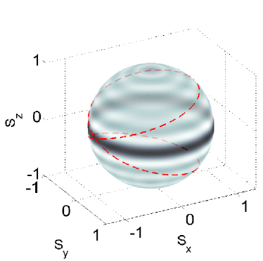
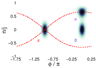
Figure 2: (Color online) An illustration of TwinFock (${n=0}$) preparation (left), and of Pi (”$\pi$”), Zero (”$0$”) and Edge (”e”) preparations (right) using Wigner plots on a sphere. The left panel is a 3D plot, while the right panel is a Mercator projection of the sphere using ${(\bm{\varphi},\bm{n})}$ coordinates.

(a)                      (b)                      (c)                     

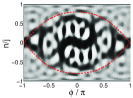
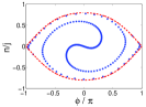
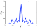
Figure 3: (Color online) The evolving quantum state of $N=40$ bosons with $u=5$ for TwinFock ($n=0$) preparation. Here and below the units are such that ${K=1}$. The time is $t=4$. (a) Wigner function of the evolved quantum state. (b) Semiclassical evolved state. (c) Occupation statistics, with the semiclassical result shown as dashed-dotted line.

(a)                                (b)                               

Figure 7: (Color online) The mean frequency of the $S_{x}(t)$ oscillations versus $u/N$ for for $N=100\,(\circ),500\,(\Box),$ and $1000\,(\diamond)$ particles. The preparations are (upper to to lower sets of data points): Zero (blue), Edge (magenta), and Pi (red). The doubled Josephson frequency $2\omega_{J}$ is marked by a dashed blue line. The theoretical predictions of Eq. (42), doubled due to mirror symmetry, are represented by red and magenta dashed lines, while Eq. (43) for ${u/N\gg 1}$ is represented by black dash-double-dotted line (there is one fitting parameter as explained there).

Figure 8: (Color online) Left: The long-time average of $S_{x}(t)$ versus $u/N$ for $N=100\,(\circ),500\,(\Box),$ and $1000\,(\diamond)$ particles. The preparations are (upper to lower sets of data points): Zero (blue), TwinFock (black), Edge (magenta), and Pi (red). The symbols are used for the quantum results and the dashed lines are the semiclassical prediction for fourty particles. Note that the scaling holds only in the Josephson regime ${1\ll u\ll N^{2}}$, and therefore, for a given $u/N$ range, becomes better for large $N$. Right: The long time RMS of $S_{x}(t)$ for the three coherent preparations (lower to upper sets): Zero (blue), Edge (magenta), and Pi (red). The implied $N^{1/4}$ scaling based on Eq. (69)) is confirmed. In the inset, the RMS of $S_{x}(t)$ for Edge ($\triangle$) and Pi ($\triangledown$) preparations is plotted versus $N$ while ${u=4}$ is fixed. The dashed lines are power-law fits that nicely agree with the predictions of Eq. (70).

References

- (1) The arXiv:1001.2120 version of this paper includes 3 extra pedagogically oriented appendices: Bosons in site system and MFT; Detailed analysis of phase space geometry in the case; The definition of a Wigner function of a spin; Concise discussion of the Rabi-Josephson oscillations in the semiclassical perspective.
- (2) D. Jaksch C. Bruder, J. I. Cirac, C. W. Gardiner, and P. Zoller, Phys. Rev. Lett. 81, 3108 (1998).
- (3) M. Greiner, O. Mandel, T. Esslinger, T. W. Hänsch, and I. Bloch, Nature (London) 415, 39 (2002).
- (4) Y. Makhlin, G. Schön, and A. Shnirman, Rev. Mod. Phys. 73, 357 (2001); R. Gati and M. K. Oberthaler, J. Phys. B 40, R61 (2007).
- (5) Gh-S. Paraoanu et al., J. Phys. B: At. Mol. Opt. Phys. 34, 4689 (2001); A. J. Leggett, Rev. Mod. Phys. 73, 307 (2001).
- (6) J. Javanainen, Phys. Rev. Lett. 57, 3164 (1986).
- (7) F. Dalfovo, L. Pitaevskii, and S. Stringari, Phys. Rev. A 54, 4213 (1996).
- (8) I. Zapata, F. Sols, and A. J. Leggett, Phys. Rev. A 57, 1050 (1998).
- (9) A. Smerzi, S. Fantoni, S. Giovanazzi, and R. S. Shenoy, Phys. Rev. Lett. 79, 4950 (1997).
- (10) F. S. Cataliotti, S. Burger, C. Fort, P. Maddaloni, F. Minardi, A. Trombettoni, A. Smerzi, and M. Inguscio, Science 293, 843 (2001).
- (11) M. Albiez, R. Gati, J. Fölling, S. Hunsmann, M. Cristiani, and M. K. Oberthaler, Phys. Rev. Lett. 95, 010402 (2005).
- (12) S. Giovanazzi, A. Smerzi, and S. Fantoni, Phys. Rev. Lett. 84, 4521 (2000).
- (13) S. Levy, E. Lahoud, I. Shomroni, and J. Steinhauer, Nature 449, 579 (2007); C. A. Sackett, Nature 449, 546 (2007).
- (14) A. J. Leggett and F. Sols, Found. Phys. 21, 353 (1998).
- (15) E. M. Wright, D. F. Walls and J. C. Garrison Phys. Rev. Lett. 77, 2158 (1996).
- (16) J. Javanainen and M. Wilkens, Phys. Rev. Lett. 78, 4675 (1997); Phys. Rev. Lett. 81, 1345 (1998).
- (17) M. Greiner, O. Mandel, T. W. Hänsch, and I. Bloch, Nature 419, 51 (2002).
- (18) G.-B. Jo et al., Phys. Rev. Lett. 98, 030407 (2007).
- (19) T. Schumm et al., Nat. Phys. 1, 57 (2005).
- (20) S. Hofferberth et al., Nature (London) 449, 324 (2007).
- (21) A. Widera, S. Trotzky, P. Cheinet, S. Fölling, F. Gerbier, I. Bloch, V. Gritsev, M. D. Lukin, and E. Demler, Phys. Rev. Lett. 100, 140401 (2008).
- (22) A. Vardi and J. R. Anglin, Phys. Rev. Lett. 86, 568 (2001); J. R. Anglin and A. Vardi, Phys. Rev. A 64, 013605 (2001).
- (23) Y. Khodorkovsky, G. Kurizki, and A. Vardi, Phys. Rev. Lett. 100, 220403 (2008); Phys. Rev. A 80, 023609 (2009).
- (24) E. Boukobza, M. Chuchem, D. Cohen, and A. Vardi, Phys. Rev. Lett. 102, 180403 (2009).
- (25) K. Smith-Mannschott, M. Chuchem, M. Hiller, T. Kottos, and D. Cohen, Phys. Rev. Lett. 102, 230401 (2009).
- (26) C. W. Gardiner and P. Zoller, Quantum Noise, 2nd ed. (Springer, New York, 2000).
- (27) M. J. Steel, M. K. Olsen, L. I. Plimak, P. D. Drummond, S. M. Tan, M. J. Collett, D. F. Walls, and R. Graham, Phys. Rev. A 58, 4824 (1998).
- (28) A. Sinatra, C. Lobo, and Y. Castin, Phys. Rev. Lett. 87, 210404 (2001); J. Phys. B: At. Mol. and Opt. Phys. 35, 3599 (2002).
- (29) I. Carusotto, Y. Castin, and J. Dalibard, Phys. Rev. A 63, 023606 (2001).
- (30) S. E. Hoffmann, J. F. Corney, and P. D. Drummond, Phys. Rev. A 78, 013622 (2008).
- (31) A. Polkovikov, Phys. Rev. A 68, 053604 (2003).
- (32) L. I. Plimak, M. Fleischhauer, M. K. Olsen, and M. J. Collett, Phys. Rev. A 67, 013812 (2003).
- (33) P. Deuar and P. D. Drummond, J. Phys. A: Math and Gen. 39, 1163 (2006); J. Phys. A: Math and Gen. 39, 2723 (2006);
- (34) L. Isella and J. Ruostekoski, Phys. Rev. A 74, 063625 (2006).
- (35) M. Hiller, T. Kottos, and T.Geisel , Phys. Rev. A 73, 061604(R) (2006); Phys. Rev. A 79, 023621 (2009).
- (36) S. L. W. Midggley, S. Wüster, M. K. Olsen, M. J. Davis, and K. V. Kheruntsyan, Phys. Rev. A 79, 053632 (2009).
- (37) P. Deuar, Phys. Rev. Lett 103, 130402 (2009).
- (38) F. Trimborn, D. Witthaut, and H. J. Korsch, Phys. Rev. A 77, 043631 (2008); Phys. Rev. A 79, 013608 (2009).
- (39) K.W. Mahmud, H. Perry, and W.P. Reinhardt, Phys. Rev. A 71, 023615 (2005).
- (40) Franzosi et al, Int. J. Mod. Phys. B 14, 943 (2000).
- (41) E. Boukobza, D. Cohen, and A. Vardi, Phys. Rev. A 80, 053619 (2009).
- (42) E.M. Graefe, H.J. Korsch, Phys. Rev. A 76, 032116 (2007); D. Witthaut, E. M. Graefe, and H. J. Korsch, Phys. Rev. A 73, 063609 (2006).
- (43) G. S. Agarwal, Phys. Rev. A. 24, 2889 (1981). J. P. Dowling, G. S. Agarwal,W. P Schleich, Phys. Rev. A 49, 4101 (1994).
- (44) J.C. Varilly and J.M. Gracia-Bondia, Annals of Physics 190, 107 (1989). C. Brif and A. Mann, J. Phys. A 31, L9 (1998).
- (45) A. Polkovnikov, S. Sachdev, and S.M. Girvin, Phys. Rev. A 66, 053607 (2002).
- (46) E. Altman and A. Auerbach, Phys. Rev. Lett. 89, 250404 (2002).
- (47) A. K. Tuchman, C. Orzel, A. Polkovnikov, and M. Kasevich, Phys. Rev. A 74, 051601 (2006).
- (48) B. Wu and Q. Niu, Phys. Rev. A 61, 023402 (2000).
- (49) J. C. Eilbeck, P. S. Lomdahl, and A. C. Scott, Physica D 16, 318 (1985).
- (50) R. L. Stratonovich, Sov. Phys. JETP 31, 1012 (1956).
- (51) D. Cohen and T. Kottos, Phys. Rev. E 63, 36203 (2001).
- (52) E. Boukobza, M. G. Moore, D. Cohen, and A. Vardi, Phys. Rev. Lett. 104, 240402 (2010).
- (53) M. Rigol, V. Dunjko, and M. Olshanii, Nature 452, 854 (2008).
- (54) Quantum Optics by M.O. Scully and M.S. Zubairy, (Cambridge University Press, 1997), p.201.
(a) (b) (c)
(a) (b)
(c) (d)