Microfield Fluctuations and Spectral Line Shapes in Strongly Coupled Two–Component Plasmas

Abstract

The spectral line shapes for hydrogen–like heavy ion emitters embedded in strongly correlated two–component electron–ion plasmas are investigated with numerical simulations. For that purpose the microfield fluctuations are calculated by molecular dynamics simulations where short range quantum effects are taken into account by using a regularized Coulomb potential for the electron–ion interaction. The microfield fluctuations are used as input in a numerical solution of the time–dependent Schrödinger equation for the radiating electron. In distinction to the standard impact and quasistatic approximations the method presented here allows to account for the correlations between plasma ions and electrons. The shapes of the Ly_α–line in Al are investigated in the intermediate regime. The calculations are in good agreement with experiments on the Ly_α–line in laser generated plasmas.

I Introduction

Measurements of emission and absorption spectra of atoms and ions are one of the most important tools in plasma diagnostics gri97 ; sal98 ; dat . They allow for investigations of the properties of various laboratory and space plasmas. In particular, spectral line shapes may be analyzed to yield a wealth of information on the plasma parameters provided, however, that the data are compared to accurate computations of the spectral line broadening.

Traditionally, in the theory of spectral line broadening in plasmas ion effects in most cases were calculated within the quasistatic approximation, while the electron perturbation was believed to satisfy the impact approximation. The description of this method (Standard Theory (ST)) is given, e.g., in Refs. gri97 ; sal98 ; dat . The separation of perturbations into ion and electron parts, in general, cannot be made without a loss of accuracy, although it is argued ale96 that in many cases it is justified. A more serious problem, however, is that each of the ion and electron parts often needs to be considered beyond the limits of the quasistatic and impact approximations. In particular, the ion motion in plasma leads to the so–called ion dynamics effects. It was first shown theoretically duf69 ; fri71 and soon found in experiments kel73 ; gru77 ; gru78 , that the ion dynamics can be responsible for significant corrections to the spectral line widths. In order to advance the calculations beyond the ST, several numerical methods have been developed. Among the first is the method developed in Ref. sta83 , where a computer code was used to simulate the ion motion along straight paths, while the electron contribution was calculated using the impact approximation. The method was further improved in Ref. sta86 by using molecular–dynamics (MD) simulations for the ions, thus accounting for interactions between the radiators and the ion perturbers. In Refs. gig87 ; heg88 ; car89 ; gig96 the motion of both ions and electrons was numerically simulated. The particle motion was simulated using straight path trajectories, which is applicable when the correlations between the perturbers and radiator are neglected. Later, the area of applicability was extended by using hyperbolic ale97 and, recently, exact paths for the perturbers (see, e.g., Refs. mar03 ; mar04 ; sta06 and references therein). In Refs. mar03 ; mar04 the model was based on one–component plasmas (OCPs) treating the full spectrum as a superposition of the electronic and ionic contributions and thus neglects the influence of the attractive interactions between electrons and ions. This is well justified for weakly coupled plasma where the ionic and electronic fields can be handled separately for spectra modeling. But there is an increasing number of experiments of interest which are far beyond such parameter regimes (see, e.g., Refs. sae99 ; eid00 ; and02 ; eid03 ). In such cases a simple superposition of the electronic and ionic fields becomes insufficient due to strong nonlinear effects and the total field in a two–component plasmas (TCP) should serve as the starting point for spectra modeling. The related microfield distribution (MFD) and the line shapes including the full attractive electron–ion interaction has thus been attracting more and more attention and has already been studied, e.g., in Refs. sad09 ; ner05 ; ner06 ; ner08 ; cal07 ; fer07 ; sta07 ; tal02 .

The present paper is the continuation of Ref. mar04 but we treat here the ions and electrons on an equal footing by concentrating on the TCP. For that purpose we perform MD simulations which span the entire range between the impact and the quasistatic approximations. We solve the time–dependent Schrödinger equation for the radiator in the fluctuating microfield generated by the plasma particles. The MD simulations in conjunction with the Schrödinger equation to study the line shapes in a TCP have been previously considered in Ref. sta06 . Our model is thus similar to that considered in sta06 but, in addition, it allows to treat the interaction of the emitted photons with radiating electron.

II MD simulations

A two–component classical plasma of electrons and ions (with the charge $Ze$) is in equilibrium with the temperature $T$ completely described by the coupling parameters $\Gamma_{\alpha\beta}$ with $\alpha$,$\beta=e$,$i$. Introducing the mean electron–electron ($a_{e}$), ion–ion ($a_{i}$) and electron–ion ($a$) distances through the relations, $a_{\alpha}^{-3}=4\pi n_{\alpha}/3$, $a^{-3}=4\pi n/3$ (where $n=n_{e}+n_{i}$ is the total plasma density with $n_{e}=Zn_{i}$) these parameters are defined as ner05 ; ner06 ; ner08

$$\Gamma_{\alpha\alpha}=\frac{q^{2}_{\alpha}e_{S}^{2}}{k_{B}Ta_{\alpha}}\ ,\quad\Gamma_{ei}=\frac{Ze_{S}^{2}}{k_{B}Ta}\ .$$ (1)

Here $q_{e}=-1$, $q_{i}=Z$, $e_{S}^{2}=e^{2}/4\pi\varepsilon_{0}$ and $\varepsilon_{0}$ is the permittivity of the vacuum.

It is well known kel63 ; deu81 that, to avoid the collapse of the classical system of electrons and ions, the Coulomb electron–ion interaction potential must be replaced by the pseudopotential with a regularized short–range behavior. In this paper we consider the electron–ion pair interaction potential $-e_{S}^{2}q_{\beta}u_{ei}(r)$, where $\beta=i,R$, $q_{R}e$ is the charge of the radiator (throughout this paper the index $R$ refers to the radiators) and

$$u_{ei}(r)=\frac{1}{r}(1-e^{-r/\delta}),$$ (2)

which is regularized at small distances. The cutoff parameter $\delta$ may be qualitatively thought of as a classical emulation of the electron thermal de Broglie length. For large distances $r>\delta$ the potential becomes Coulomb, while for $r<\delta$ the Coulomb singularity is removed and $u_{ei}(0)=1/\delta$. By this the short range effects based on the uncertainty principle are included tal02 ; kel63 ; deu81 .

For a classical description of a plasma the electron degeneracy parameter $\Theta_{e}$, i.e., the ratio of the thermal energy and the Fermi energy must fulfill $\Theta_{e}=k_{B}T/E_{F}>1$. Since an ion is much heavier than an electron this condition is usually fulfilled for ions. Therefore one can expect that the regularization given by Eq. (2) is less important for ions than for electrons. Furthermore, scattering of any two particles is classical for impact parameters that are large compared to the de Broglie wavelengths $\lambdabar_{\alpha\beta}=(2\pi\hbar^{2}/\mu_{\alpha\beta}k_{B}T)^{1/2}$, where $\mu_{\alpha\beta}$ is the reduced mass of the particles $\alpha$ and $\beta$. Typical impact parameters are given by the Landau lengths, $\lambda_{L\alpha\beta}=e_{S}^{2}|q_{\alpha}q_{\beta}|/k_{B}T$. Its ratio to the de Broglie wavelengths is given by

$$\sigma_{\alpha\beta}=\frac{\Gamma_{ei}\left|q_{\alpha}q_{\beta}\right|}{Z}\frac{a}{\lambdabar_{\alpha\beta}}\ .$$ (3)

Note that $\sigma_{ee}<\sigma_{ei}\ll\sigma_{ii}$. A classical description of the scattering events in the TCP is valid if $\sigma_{ee}>1$.

A collective length scale is given by the Debye screening radius, for a TCP $\lambda_{D}=a/(3\Gamma_{ei})^{1/2}$. The plasma frequencies for electrons and ions $\omega_{p\alpha}=(4\pi q_{\alpha}^{2}n_{\alpha}e_{S}^{2}/m_{\alpha})^{1/2}$ with $\alpha=e,i$ set the collective time scales $\omega_{pe}^{-1}$ and $\omega_{pi}^{-1}$ for electronic and ionic subspecies, respectively. Due to their large mass ratio the electrons and the ions move on very different timescales. Moreover, for a nonrelativistic treatment the thermal energy of the particles must be smaller than their rest energy. Since this is important only for electrons we require that $k_{B}T\ll m_{e}c^{2}$. Also the validity of the dipole approximation for plasma–radiator interaction used in Sec. III requires that the characteristic length scale of the plasma microfield must be larger than the effective atomic length scale $a_{Z}=a_{B}/Z$, where $a_{B}$ is the Bohr radius. Since this length is $\simeq a$ the dipole approximation is valid when $a\gtrsim a_{Z}$ which is usually fulfilled for heavy radiators. In this paper we consider hydrogen–like ions as radiators in a completely ionized TCP, i.e. we assume that $q_{R}=Z_{R}-1$, where $Z_{R}e$ is the charge of the nucleus of the radiating ion.

Let us now briefly discuss the limitations of the MD model arising from the classical description of the electrons, i.e., from the neglect of the quantum effects in the short–range electron–ion interaction. As shown in Ref. fis01 two constraints on the parameter $\delta$ determining the regularized potential (2) must be considered. In the parameter regime when a significant fraction of the simulated electrons is found in the quasibound states the simulated $Z$ and $Z_{R}$ are effectively reduced and the MD simulations are not adequate. Thus, the parameter $\delta$ must be chosen large enough to suppress the formation of the classical bound states of electrons. On the other hand the condition $\delta\lesssim a$ must be fulfilled so not to affect the free electron density at $r\sim a$. The probability to found an electron within a volume $r\lesssim\delta$ from an ion is estimated by $W\simeq(4\pi\delta^{3}/3)n_{e}g_{ei}(0)$, where the electron–ion radial distribution function $g_{ei}(r)$ can be approximated by the nonlinear Debye–Hückel expression $g_{ei}(r)\simeq\exp{[\beta_{e}Ze^{2}_{S}u_{ei}(r)]}$ (see, e.g., Refs. ner05 ; tal02 ) with $\beta_{e}=1/k_{B}T$. Note that in the case when $Z\gg 1$, the capture of an electron on the quasibound orbit reduce the effective $Z$ and $\Gamma_{ei}$ for the next one, so a significant fraction of electrons can stay free even for $\Gamma_{ei}a/\delta\gg 1$. The minimal value of $W(\delta)$ occurs at $\delta=\Gamma_{ei}a/3$. It is thus clear that for $\Gamma_{ei}\gtrsim 0.5$ the capture of the electrons onto classical orbits becomes important and the significant contribution from the classically bound electrons cannot be avoided in the MD models with point–like classical electrons.

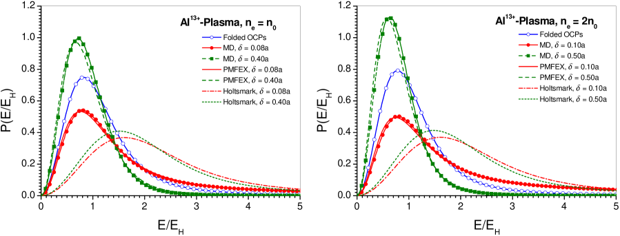
Figure 1: Normalized electric microfield distributions for Al¹³⁺ TCPs with $k_{B}T=500$ eV, $n_{e}=n_{0}$, $\Gamma_{ee}=0.037$, $\Gamma_{ii}=2.65$ (left) and $n_{e}=2n_{0}$, $\Gamma_{ee}=0.046$, $\Gamma_{ii}=3.34$ (right) as a function of the electric field in units of $E_{H}$, Eq. (4), for different values of $\delta$. The lines with and without symbols represent the MFD from the MD simulations and PMFEX model, respectively. The open circles are the MFD obtained from the folding of an electronic and an ionic OCP, see Eq. (5). The Holtsmark distributions for a TCP (see Ref. ner05 ) are shown as dot–dashed and dotted lines. (Online color:www.cpp-journal.org).

The electric microfield distribution (MFD) $P(E)$ plays a central role for the line shape. Models for this distribution exist in the limits of an ideal plasma hol19 , a weakly coupled plasma hoo68 and for very strongly coupled plasmas may47 . For intermediate cases an effective independent–particle model known as Adjustable Parameter Exponential (APEX) approximation has been developed in Refs. igl83 ; duf85 ; boe87 for an ionic OCP. It rests essentially on the pair distribution function and has been tested by comparison with MD and Monte–Carlo simulations. Recently in Refs. ner05 ; ner06 ; ner08 we have suggested the theoretical models named PMFEX (Potential of Mean Force Exponential approximation) and PMFEX+ which turn out to be a very reliable approaches for calculating the MFD of a TCP with attractive interaction. In order to cover the entire range from small to large plasma parameters we use here classical MD simulations which have been described in detail in Ref. zwi99 (see also Refs. ner05 ; ner06 ; ner08 ). As an example the normalized MFDs from PMFEX and MD are compared in Fig. 1 where the electric microfields are scaled in units of the Holtsmark field $E_{H}$ for a TCP (see ner05 for details)

$$E_{H}=\frac{C\mathcal{Z}e}{4\pi\varepsilon_{0}a^{2}},\qquad\mathcal{Z}=\left[\frac{Z\left(1+Z^{1/2}\right)}{Z+1}\right]^{2/3}$$ (4)

with an effective charge $\mathcal{Z}$ and $C=(8\pi/25)^{1/3}$. These distributions were obtained from ensembles of fields taken at a charged reference point which is chosen to be one of the plasma ions.

The MFDs for Al¹³⁺ TCP with temperature $500$ eV and with coupling parameters $\Gamma_{ee}=0.037$, $\Gamma_{ii}=2.65$ and $\Gamma_{ee}=0.046$, $\Gamma_{ii}=3.34$ are shown in left and right panels of Fig. 1, respectively, for different values of $\delta$. The density of plasma electrons is measured in units of $n_{0}=5\times 10^{23}$ cm^-3. The dot–dashed and dotted curves are, for comparison, the Holtsmark MFDs for a TCP with regularized Coulomb potential. Here these MFDs depend on $Z$ and $\delta$ as discussed in ner05 . To demonstrate the importance of the attractive interactions we also plotted the MFDs $P_{0}(E)$ resulting from the corresponding electronic and ionic OCPs with $\Gamma_{ee}$ and $\Gamma_{ii}$, respectively (open circles). To that end the distribution $Q_{0}(\mathbf{E})=P_{0}(E)/(4\pi E^{2})$ of the total field $\mathbf{E}=\mathbf{E}_{1}+\mathbf{E}_{2}$ is calculated as

$$Q_{0}(\mathbf{E})=\int d\mathbf{E}_{1}d\mathbf{E}_{2}\delta\left(\mathbf{E}-\mathbf{E}_{1}-\mathbf{E}_{2}\right)Q_{e}(\mathbf{E}_{1})Q_{i}(\mathbf{E}_{2})$$ (5)

from the MFD of the ionic OCP at a charged point $Q_{i}(\mathbf{E}_{2})$ and of the electronic OCP at a neutral reference point $Q_{e}(\mathbf{E}_{1})$. The distribution $Q_{0}(\mathbf{E})$ thus represents the MFD in a TCP assuming that the ion–electron attractive interaction is absent. Here $Q_{e}(\mathbf{E}_{1})$ and $Q_{i}(\mathbf{E}_{2})$ are taken from MD simulations of an OCP. As the thermal motion of the particles is suppressed with increasing coupling the distributions $P(E)$ and the mean electric fields are shifted towards smaller values as shown in Fig. 1. This figure also shows the importance of the attractive interactions in plasmas. The behavior of the MFD with respect to the variation of the parameter $\delta$ is particularly noteworthy. For fixed coupling parameters the maximum of the MFD shifts only slightly to lower field strengths $E$ with increasing $\delta$ (Fig. 1), while the maximum itself increases with $\delta$. This is related to the largest possible single–particle field $|E_{e}(0)|=e/(8\pi\varepsilon_{0}\delta^{2})$, which an electron can produce at the ion. Thus the nearest neighbor electronic MFD vanishes for electric fields larger than $|E_{e}(0)|$, and smaller $\delta$ will result in larger contributions to $P(E)$ at higher fields $E$ with a corresponding reduction of $P(E)$ at small fields. Therefore, the formation of the tails in the MFD and enhancement of the electric microfield at small $\delta$ may have important influence on the spectral line shapes of the radiating particles. Further examples for charged and neutral radiators, together with a detailed discussion of the limits of the PMFEX treatment at increasing coupling, are given in Refs. ner05 ; ner06 ; ner08 .

III Wave equation for a radiator

In this section we describe the solution of the wave equation for a hydrogen–like ion coupled to the time–dependent electric microfield. The microfield fluctuations in the plasma are calculated by the MD simulations as discussed in Sec. II.

We consider a hydrogen–like ion in a time–dependent electric microfield. The Hamiltonian is the sum of $\hat{H}_{0}$ describing the unperturbed ion and a dipole term $\hat{H}_{\mathrm{int}}=e\mathbf{r}\cdot\mathbf{E}(t)$ for the interaction between the bound electron (distance $\mathbf{r}$ from nucleus) and the microfield $\mathbf{E}(t)$,

$$\hat{H}=\hat{H}_{0}+\hat{H}_{\mathrm{int}}\ .$$ (6)

The electron moves in the potential of a nucleus with charge $Z_{R}e$. In the present application it turns out that it suffices to start from the non–relativistic Schrödinger equation

$$\hat{H}_{0}\left|\alpha\right\rangle=\left(\frac{\hat{\mathbf{p}}^{2}}{2m_{e}}-\frac{Z_{R}e_{S}^{2}}{r}\right)\left|\alpha\right\rangle=\hbar\omega_{\alpha}\left|\alpha\right\rangle$$ (7)

for the time–independent electronic state $|\alpha\rangle$ with energy $E_{\alpha}=\hbar\omega_{\alpha}$. Here $\hat{\mathbf{p}}$ is the momentum operator and $\alpha$ is a multiindex including radial, angular momentum and spin quantum numbers. The present calculations are done in the configuration space corresponding to the solutions of Eq. (7). In order to discretize the continuum a boundary condition $\langle\mathbf{r}|\alpha\rangle=0$ is imposed at a radius $r=R_{0}$, which is chosen sufficiently large in order to avoid an influence on the final results. The radial wave functions with this boundary condition are still confluent hypergeometric functions, but the radial quantum numbers of bound states are not integers any more mar03 . In order to obtain a finite basis the (former) continuum states are cut off at sufficiently large quantum numbers. Alternatively the continuum could be handled by forming wave packets with a width that must be adjusted appropriately mul94 . In Refs. mar03 ; mar04 the time–dependent equation $\hat{H}\Psi(t)=i\hbar\dot{\Psi}(t)$ with the Hamiltonian (6) has also been solved on a grid for the electron wave function cal00 ; rei00 . This is more advantageous for the description of the continuum and it is easier to implement the interactions between the radiator and the plasma particles beyond the dipole term in Eq. (6). On the other hand spatially extended states require very large simulation boxes. Quite generally in the present context the solution on the grid is more expensive numerically than working in configuration space. We adopted the latter for the subsequent calculations.

At high $Z_{R}$ relativistic corrections must be considered and also the spin should be treated as a dynamical variable. It turns out that in the cases considered here it suffices to include the first–order fine–structure shift fri90

$$\Delta E_{nlj}=-\frac{Z_{R}^{2}\alpha_{S}^{2}\left|E_{n}\right|}{n}\left(\frac{1}{\gamma_{lj}}-\frac{3}{4n}\right)\ ,$$ (8)

where $\gamma_{lj}=j+1/2$ and $\gamma_{lj}=1$ at $l\geqslant 1$ and $l=0$, respectively. Here $n$ is the principal quantum number of the hydrogen–like ion, $E_{n}=-Z_{R}^{2}E_{B}/n^{2}$ is the corresponding energy ($E_{B}=e_{S}^{2}/2a_{B}$ is the Bohr energy), $j=l\pm 1/2$ is the total angular momentum quantum number and $\alpha_{S}\simeq 1/137$ is the Sommerfeld constant.

The dipole interaction $e\mathbf{r}\cdot\mathbf{E}(t)$ between the radiator and the plasma is time–dependent and possibly strong. Going beyond the second order treatment of Ref. jun00 we use the interaction picture with the unperturbed basis states given by Eq. (7). The time–dependent Schrödinger equation with the total Hamiltonian (6) can be solved using Dirac’s method. The perturbed electron wave function is represented as a sum of wave functions of the unperturbed Hamiltonian with time–dependent coefficients $c_{\alpha}(t)$

$$\Psi(t)=\sum_{\alpha}c_{\alpha}(t)e^{-i\omega_{\alpha}t}\left|\alpha\right\rangle\ .$$ (9)

A substitution of Eq. (9) into the time–dependent Schrödinger equation and orthogonality of the spatial wave functions, i.e., $\langle\alpha|\beta\rangle=\delta_{\alpha\beta}$, gives the set of coupled ordinary and linear differential equations

$$\dot{c}_{\alpha}(t)=-\frac{ie}{\hbar}\mathbf{E}\left(t\right)\cdot\sum_{\beta}e^{i\omega_{\alpha\beta}t}c_{\beta}(t)\left\langle\alpha\left|\mathbf{r}\right|\beta\right\rangle$$ (10)

which is solved iteratively. Here $\hbar\omega_{\alpha\beta}$ is the transition energy between atomic states $\alpha$ and $\beta$, i.e., $\omega_{\alpha\beta}=\omega_{\alpha}-\omega_{\beta}$. Within the dipole approximation the transition rate per unit time and energy interval $\mathcal{I}(\omega)$ for the emission of photons is proportional to the power spectrum of the dipole operator jac98 . It is defined as the square of the absolute value of the Fourier transform of the expectation value of the dipole operator. Hence we introduce

$$\mathcal{I}\left(\omega\right)=\frac{2e_{S}^{2}\omega^{3}}{3\pi c^{3}\hbar^{2}\tau}\left|\int_{0}^{\tau}\mathbf{d}(t)e^{i\omega t}dt\right|^{2}$$ (11)

with $\tau\to\infty$ and the expectation value of the dipole moment

$$\mathbf{d}(t)=\sum_{\beta,\alpha}e^{i\omega_{\beta\alpha}t}c_{\beta}^{\ast}(t)c_{\alpha}(t)\left\langle\beta|\mathbf{r}|\alpha\right\rangle.$$ (12)

Let us now consider a transition $\alpha\to g$ downwards to a state $|g\rangle$ which is nearly filled, i.e. $c_{\beta}(t)=\delta_{\beta g}$. Then the dipole moment in Eq. (12) is calculated with respect to the state $|g\rangle$ and

$$\mathcal{I}\left(\omega\right)=\frac{2e_{S}^{2}\omega^{3}}{3\pi c^{3}\hbar^{2}\tau}\left|\sum_{\alpha}\left\langle g\left|\mathbf{r}\right|\alpha\right\rangle\int_{0}^{\tau}c_{\alpha}(t)e^{i\left(\omega-\omega_{\alpha g}\right)t}dt\right|^{2}.$$ (13)

Our numerical model includes also the interaction $\hat{H}_{\mathrm{e\gamma}}$ of the radiating electron with the emitted photons which, however, has been neglected in Eq. (6). In this case as shown in Refs. mar03 ; mar04 the total radiated power given in Eq. (13) is underestimated for the excited radiators where $|c_{g}|^{2}<1$. This can be compensated by dividing through the time–averaged occupation probability of the lower state

$$\mathcal{I}\left(\omega\right)\to\frac{\mathcal{I}\left(\omega\right)}{\langle\left|c_{g}(t)\right|^{2}\rangle_{t}}\ .$$ (14)

The subsequent calculations will be done in this dipole power spectrum approximation (DPSA). We have tested the validity of this approximation in the wide range of plasma and radiator parameters by comparing explicitly $\mathcal{I}(\omega)$ with the spectrum obtained from the total Hamiltonian $\hat{H}^{\prime}=\hat{H}_{0}+\hat{H}_{\mathrm{int}}+\hat{H}_{\mathrm{e\gamma}}$. We have found that in the parameter regime considered in Sec. IV the DPSA is justified as the emission of radiation through the interaction $\hat{H}_{\mathrm{e\gamma}}$ changes the occupation probabilities of the radiator’s states on a much slower scale than the fluctuating electric microfields. However, our preliminary results show that the electron–photon interaction $\hat{H}_{\mathrm{e\gamma}}$ may have an important contribution to the wings of the line especially in the case of light emitters. We intend to take up further studies on this issue in a separate paper.

At this stage we have neglected the feedback of the radiator’s excitation to the plasma. In this respect the plasma particles move as if they had an infinite mass. As they have a finite velocity it appears as if the radiating electron is embedded in a plasma of infinite temperature. Accordingly the time evolution of the total system will lead to an equal population of all electronic states. As the time–dependent feedback could be implemented only at a very great expense in the MD simulations we enforce a canonical equilibrium state of the plasma and the radiating electron by modifying the interaction in Eq. (10) according to

$$e\mathbf{r}\cdot\mathbf{E}(t)\rightarrow e^{-\beta_{e}\hat{H}_{0}/2}e\mathbf{r}\cdot\mathbf{E}(t)e^{\beta_{e}\hat{H}_{0}/2}.$$ (15)

The time–dependent equation (10) describing the coupling of the microfield to the radiator is then solved for an ensemble of typically thirty independent microfields which yields the mean emission as well as the statistical error.

IV Results

Using the theoretical background introduced so far we present in this Section calculations of the shape of the Ly_α–line of Al¹²⁺ radiating ion embedded in a Al¹³⁺–TCP in a wide range of plasma parameters. As we have mentioned in Sec. III for heavy ions the relativistic corrections, i.e. the fine structure of the levels must be accounted for. Using the fine structure shift in Eq. (8) the unperturbed Ly_α transition energy becomes

$$\hbar\omega_{\mathrm{Ly}_{\alpha}}=\frac{3}{4}Z_{R}^{2}E_{B}\left(1+C_{j}Z_{R}^{2}\alpha_{S}^{2}\right)$$ (16)

with $C_{1/2}=\frac{11}{48}$, $C_{3/2}=\frac{5}{16}$ and for Al¹²⁺ ions $\hbar\omega_{\mathrm{Ly}_{\alpha}}\simeq 1728.1$ eV and $\hbar\omega_{\mathrm{Ly}_{\alpha}}\simeq 1729.4$ eV with $j=1/2$ and $j=3/2$, respectively.

We start from the line as it is broadened by the Al¹³⁺ ions and electrons in the plasma. Then we fold with the weighted fine structure shift Eq. (8) which is $\hbar\Delta\omega\simeq 1.29$ eV according to

$$\mathcal{I}_{\mathrm{LS}}(\omega)=\frac{1}{3}\mathcal{I}\left(\omega+\frac{2}{3}\Delta\omega\right)+\frac{2}{3}\mathcal{I}\left(\omega-\frac{1}{3}\Delta\omega\right)$$ (17)

and account for the Doppler effect gri97 ; sal98 which broadens a line with the unperturbed frequency $\omega_{0}$ according to a Gaussian distribution

$$\mathcal{D}\left(\Delta\omega\right)=\frac{1}{\sqrt{2\pi}\sigma}\exp\left[-\frac{1}{2}\left(\frac{\Delta\omega}{\sigma}\right)^{2}\right],$$ (18)

where $\Delta\omega=\omega-\omega_{0}$ and

$$\sigma^{2}=\frac{\omega_{W}^{2}}{8\ln 2}=\omega_{0}^{2}\frac{k_{B}T}{M_{R}c^{2}}.$$ (19)

Here $\hbar\omega_{W}$ is the full width at half maximum (FWHM) of the line and $M_{R}$ is the radiating ion mass. Some values of FWHM $\hbar\omega_{W}$ for aluminum are shown in Table 1. Finally, we fold to account for the experimental resolution.

Table 1: Doppler broadening (FWHM) of the Ly_α–line in an Al plasma.

$k_{B}T$ (eV)	10	102	$5\times 10^{2}$	103	104	$10^{5}$
FWHM (eV)	0.08	0.26	0.57	0.81	2.57	8.12

We discuss now the simulated Ly_α–line profiles at solid state densities $n_{0}\leqslant n_{e}\leqslant 4n_{0}$ and at $k_{B}T=500$ eV. Some results for the Ly_α–line shape without Doppler broadening and LS coupling are shown in Figs. 2-5. In all cases the ratio $a_{Z}/a\ll 1$ is small and the use of the dipole approximation in Eq. (6) is fulfilled. The line broadening and shift towards lower photon energies (redshift) is clearly visible in Fig. 2, which shows the line profile at fixed temperature 500 eV and different densities. Here the regularization parameter $\delta=\lambdabar_{ei}$ is determined as the thermal wavelength. With increasing density the influence of the plasma effects on the line shape becomes more pronounced. At very large densities from $n_{e}=2.6n_{0}$ (dashed line) and up to the value $n_{e}=4n_{0}$ (dash–dotted line) there is hardly any broadening and the line is only redshifted towards lower photon energies by the plasma effects. In this high density regime the fluctuating electric fields become sufficiently strong to cause asymmetric shapes due to nonlinear coupling.

To gain more insight we now fix the plasma temperature (500 eV) and the density ($n_{e}=n_{0}$) and show in Fig. 3 the line profile for different regularization parameters $\delta$ (the lines without symbols), $\delta=0.08a$ (solid line), $\delta=0.1a$ (dashed line) and $\delta=0.4a$ (dotted line). Here the thermal wavelengths of the electrons are chosen as the relevant lengths $\delta$ at which a smoothing of the ion–electron interaction due to quantum diffraction becomes effective. For comparison we also calculate the line shapes for non–isothermic plasma with different electronic and ionic temperatures $T_{e}=500$ eV and $T_{i}=50$ eV, respectively (the lines with symbols). As shown in Fig. 3 the width of the lines decreases with increasing parameter $\delta$, i.e. by ”softening” of the ion–electron interaction. Besides, keeping the electron temperature unchanged and decreasing the ionic temperature leads to an additional broadening of the lines and this is visible for more Coulomb–like interactions with small $\delta$.

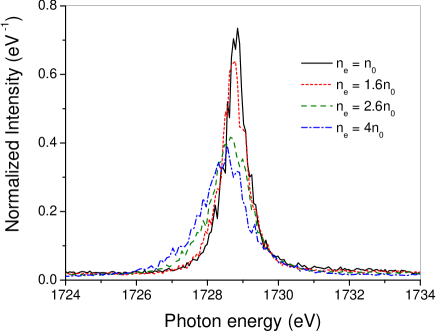
Figure 2: Simulated Ly_α–spectra of a Al¹²⁺ radiating ion embedded in a Al¹³⁺-TCP of a temperature of 500 eV and solid state densities $n_{e}=n_{0}$ (solid line), $n_{e}=1.6n_{0}$ (dotted line), $n_{e}=2.6n_{0}$ (dashed line) and $n_{e}=4n_{0}$ (dash-dotted line). The spectra are normalized to the area under the curves. (Online color:www.cpp-journal.org).

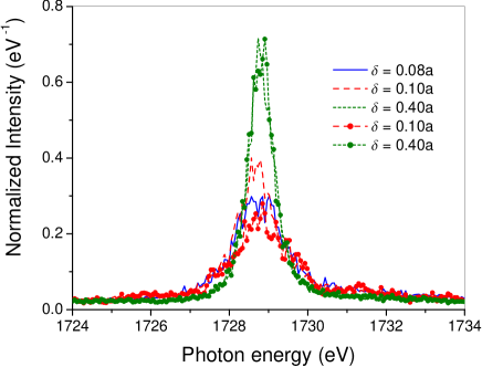
Figure 3: Simulated Ly_α–spectra of a Al¹²⁺ radiating ion embedded in a Al¹³⁺-TCP of a density of $n_{e}=n_{0}$. The lines without and with symbols correspond to the equilibrium ($T_{e}=T_{i}=500$ eV) and non-equilibrium ($T_{e}=500$ eV, $T_{i}=50$ eV) TCPs, respectively. The regularization parameter is $\delta=0.08a$ (solid line), $\delta=0.1a$ (dashed lines) and $\delta=0.4a$ (dotted lines). The spectra are normalized to the area under the curves. (Online color:www.cpp-journal.org).

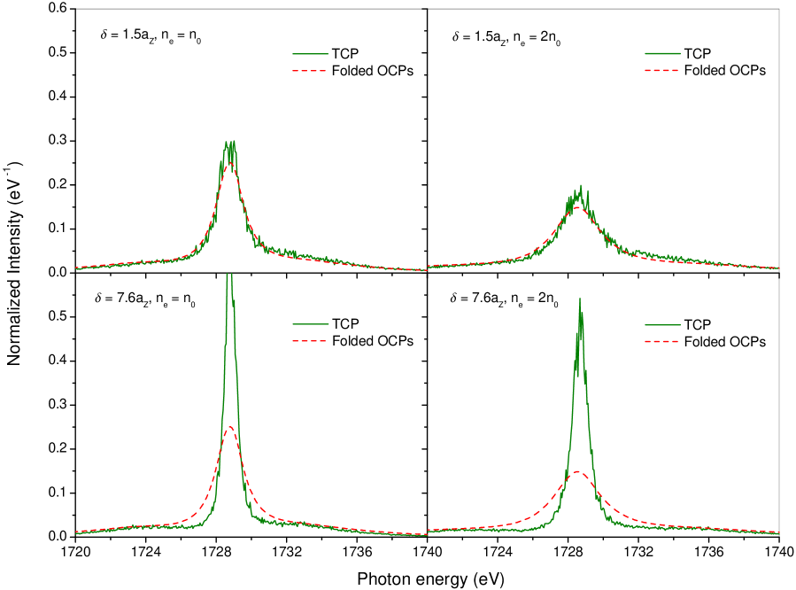
Figure 4: Simulated Ly_α–spectra of a Al¹²⁺ radiating ion embedded in a Al¹³⁺–TCP (solid lines) of a temperature of 500 eV and solid state densities $n_{e}=n_{0}$ (left panels) and $n_{e}=2n_{0}$ (right panels). The spectra are normalized to the area under the curves. The parameter $\delta$ is $1.5a_{Z}$ and $7.6a_{Z}$ in the top and bottom panels, respectively. The dashed lines are the spectra obtained from the folding of an electronic and an ionic OCP. (Online color:www.cpp-journal.org).

In Fig. 4 we put together the results obtained for two values of plasma densities ($n_{0}$ and $2n_{0}$) and the parameter $\delta$. In the top and bottom panels we take $\delta=1.5a_{Z}$ and $\delta=7.6a_{Z}$, respectively, where $a_{Z}$ is the effective Bohr radius of Al¹²⁺. Note that for two plasma densities $n_{0}$ and $2n_{0}$ the chosen values of $\delta$ in units of $a_{Z}$ are equivalent to $0.08a$, $0.1a$ and $0.4a$, $0.5a$, respectively, in units of the Wigner–Seitz radius $a$ of a TCP. We also demonstrate the influence of the electron–ion attractive interaction on the spectral line shapes plotting the spectra $\mathcal{I}_{0}(\omega)$ resulting from a superposition of the electronic and ionic OCPs (dashed lines). $\mathcal{I}_{0}(\omega)$ is calculated by folding the spectra $\mathcal{I}_{e}(\omega)$ and $\mathcal{I}_{i}(\omega)$ which are obtained from simulations of the radiative transitions of a radiator embedded in an electronic OCP and of the ionic OCP, respectively. The microfields $\mathbf{E}(t)$ in an electronic and ionic OCPs are simulated at a neutral and charged reference points, respectively. The spectrum $\mathcal{I}_{0}(\omega)$ thus represents the line shape in a TCP assuming that the ion–electron attractive interaction is switched off. As shown in Fig. 4 the width of the line now turns out to be highly sensitive to both the choice of $\delta$ and the density $n_{e}$, with a much stronger dependence on $n_{e}$ for smaller $\delta$. The influence of the high–electric field tails in the MFDs at small $\delta$ on the spectral lines is now clearly shown in Fig. 4. Smaller $\delta$ results in higher electric fields which broaden the spectral lines and reduce the peak intensity. More precisely we observed that the line width behave approximately as $\hbar\Delta\omega\sim n_{e}/\delta$.

In the following we will compare our calculations with the results of experiments performed in Garching and02 where an Al plasma is created by the irradiation of the target with laser pulses of 150 fs duration at an intensity of a few $10^{17}$ W/cm². The systematic investigations carried out in Refs. mar03 ; mar04 show that the standard (quasistatic and impact) approximations become doubtful if the plasma density reaches that of the solid state. In the last years experiments have approached this regime, see, e.g., sae99 ; eid00 ; and02 . We note that the theoretical model discussed so far assume a homogeneous equilibrium plasma. Obviously this is not the state in which the laser leaves the target after the irradiating pulse. In particular self–absorption due to plasma inhomogeneities leads to an additional line broadening which is difficult to analyze. Fortunately there has been considerable experimental progress to reduce the self–absorption and02 .

Earlier experiments on the Ly_α–line in Al¹²⁺ at solid state density sae99 ; eid00 were subject to self–absorption in the cooler and less dense surface regions of the target. This can be prevented by using thin (to reduce absorption) target layers with sharp boundaries (to enhance homogeneity). For that purpose a 25 nm Al target layer was embedded in solid carbon at depths ranging from $d=25$ nm to $d=400$ nm and02 . With increasing depth the expansion of the Al layer is suppressed and the homogeneity of the Al plasma is improved. In Fig. 5 we compare our simulations with the experimental results (filled circles) for $d=400$ nm and $k_{B}T=500$ eV from which the underground has been subtracted. The fine structure and the Doppler broadening are taken into account as described above. Then the simulated Ly_α–lines are folded with the experimental resolution (0.9 eV, FWHM) and compared with the experimental line assuming densities $5\times 10^{23}$ cm^-3 (dashed line) and $10^{24}$ cm^-3 (thin solid line). At these two densities the plasma parameters for the Al¹³⁺–TCP are $\Gamma_{ii}=2.65$, $\Gamma_{ee}=0.04$ and $\Gamma_{ii}=3.34$, $\Gamma_{ee}=0.05$, respectively. All curves in Fig. 5 are normalized to the peak intensity. Finally, the position of the simulated line must be redshifted by 2 eV. This is the dense plasma line shift (DPLS) Ref. gri97 due to the screening of the electron–nucleus interaction by hot background electrons. Assuming a Debye–screened interaction instead of the $r^{-1}$–Coulomb potential first–order perturbation theory yields a shift of the required magnitude. A comparison of the two simulated curves in Fig. 5 allows to conclude that the remaining uncertainty in the determination of the density of the target is of order $10^{23}$ cm^-3. Our results show that the quantum mechanics of close electron–ion collisions is important over and above the plasma redshift. If the quantum diffraction parameter $\delta$ is fixed at physically reasonable values near the effective Bohr radius $a_{Z}$, our calculations favor a somewhat larger density than $n_{0}$ as proposed in Ref. and02 . Clearly a more quantum mechanical treatment of the electron component in the plasmas is desirable.

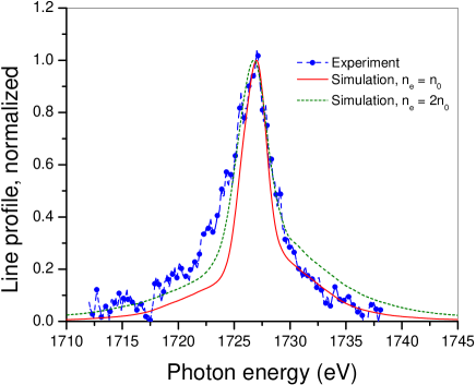
Figure 5: Comparison of the experimental line and02 (filled circles) with our simulation results (dashed and solid lines), i.e. with the solid curves from the top panels of Fig. 4 after taking into account the Doppler broadening, the LS-coupling, the experimental resolution and a redshift (see text). The experimental line is subtracted by the underground. Here the curves are normalized to the peak intensity. (Online color:www.cpp-journal.org).

V Conclusions

In this paper we have presented a model for spectral lines that works without some assumptions which underly the conventional impact and quasi–static approximations. In particular we (i) consider two–component plasma (TCP) with attractive interactions between electrons and ions, (ii) account for the strong Coulomb correlations between plasma particles, (iii) account for radiator states including the continuum, which are not directly involved in the transition, (iv) allow for a non–perturbative treatment.

We have compared our model with recent experiments on Al targets and found good agreement for the Ly_α–transitions. The more exact treatments beyond the standard approximations will become highly desirable in connection with experiments at higher densities and temperatures at the planned (X)FEL facilities.

A critical discussion of our results suggests further improvements. (i) The dipole approximation in Eq. (6) for the interaction of the microfield with the radiator suffices for the present experiments and02 . In even denser plasmas one must account for close collisions between the radiator and the plasma particles with a quadrupole term in the expansion of the interaction and finally with an exact treatment jun00 . (ii) Relativistic and spin effects beyond the simple fine structure given by Eq. (8) can be taken into account by treating the radiator with the Dirac equation mul94 . (iii) The major He–like satellite is well separated from the Ly_α–line in the experiment and02 . However, there will be closer satellites due to spectator electrons in higher configurations, which may affect the ”red” shoulder of the line. For spectators in the continuum this effect merges into the DPLS. The satellites impose a challenge as they offer an additional tool to determine the temperature of the plasma, see, e.g. Ref. sal98 . For that purpose one has to solve the multi–electron wave equation, for example in the relativistic case the Dirac equation dya89 . (iv) At high densities of the laser–produced plasmas the self–absorption is likely to occur. In general, the consideration of radiative transfer in dense plasmas is involved. To estimate the effect of the self–absorption in the calculation of the line profile one–dimensional monolayer model can be used which has already been successfully applied in Ref. lor08 (see also references therein).

- (1) H.R. Griem, Principles of Plasma Spectroscopy (Cambridge University Press, Cambridge, 1997).
- (2) D. Salzmann, Atomic Physics in Hot Plasmas (Oxford University Press, New York, 1998).
- (3) See databases of bibliographic references on the Internet at http://physics.nist.gov/PhysRefData/Linebr/ html/reffrm0.html [J. R. Fuhr, A.E. Kramida, H.R. Felrice, and K. Olsen (unpublished)].
- (4) S. Alexiou, Phys. Rev. Lett. 76, 1836 (1996).
- (5) J.W. Dufty, Phys. Rev. 187, 305 (1969); Phys. Rev. A 2, 534 (1970).
- (6) U. Frisch and A. Brissaud, J. Quant. Spectrosc. Radiat. Transfer 11, 1753 (1971).
- (7) D.E. Kelleher and W.L. Wiese, Phys. Rev. Lett. 31, 1431 (1973).
- (8) K. Grützmacher and B. Wende, Phys. Rev. A 16, 243 (1977).
- (9) K. Grützmacher and B. Wende, Phys. Rev. A 18, 2140 (1978).
- (10) R. Stamm, E.W. Smith, and B. Talin, Phys. Rev. A 30, 2039 (1983).
- (11) R. Stamm, B. Talin, E.L. Pollock, and C.A. Iglesias, Phys. Rev. A 34, 4144 (1986).
- (12) M.A. Gigosos and V. Cardenoso, J. Phys. B 20, 6006 (1987).
- (13) G.C. Hegerfeld and V. Kesting, Phys. Rev. A 37, 1488 (1988).
- (14) V. Cardenoso and M.A. Gigosos, Phys. Rev. A 39, 5258 (1989).
- (15) M.A. Gigosos and V. Cardenoso, J. Phys. B 29, 4795 (1996).
- (16) S. Alexiou, A. Calisti, P. Gauthier, L. Klein, E. Leboucher–Dalimier, R.W. Lee, R. Stamm, B. Talin, J. Quant. Spectrosc. Radiat. Transfer 58, 399 (1997).
- (17) J. Marten, thesis, Erlangen University, Erlangen (2003).
- (18) J. Marten and C. Toepffer, Eur. Phys. J. D 29, 397 (2004).
- (19) E. Stambulchik and Y. Maron, J. Quant. Spectrosc. Radiat. Transfer 99, 730 (2006).
- (20) A. Saemann et al., Phys. Rev. Lett. 82, 4843 (1999).
- (21) K. Eidmann et al., J. Quant. Spectrosc. Radiat. Transfer 65, 173 (2000).
- (22) U. Andiel, et al., Europhys. Lett. 60, 861 (2002).
- (23) K. Eidmann et al., J. Quant. Spectrosc. Radiat. Transfer 81, 133 (2003).
- (24) S.P. Sadykova, W. Ebeling, I. Valuev, and I.M. Sokolov, Contrib. Plasma Phys. 49, 76 (2009); ibid. 49, 388 (2009).
- (25) H.B. Nersisyan, C. Toepffer, and G. Zwicknagel, Phys. Rev. E 72, 036403 (2005).
- (26) H.B. Nersisyan and G. Zwicknagel, J. Phys. A: Math. and General 39, 4677 (2006).
- (27) H.B. Nersisyan, D.A. Osipyan, and G. Zwicknagel, Phys. Rev. E 77, 056409 (2008).
- (28) A. Calisti, T. del Río Gaztelurrutia, and B. Talin, High Energy Density Phys. 3, 52 (2007).
- (29) S. Ferri, A. Calisti, C. Mossé, B. Talin, M.A. Gigosos, and M.A. González, High Energy Density Phys. 3, 81 (2007).
- (30) E. Stambulchik, D.V. Fisher, Y. Maron, H.R. Griem, and S. Alexiou, High Energy Density Phys. 3, 272 (2007).
- (31) B. Talin, A. Calisti, and J. Dufty, Phys. Rev. E 65, 056406 (2002); B. Talin, A. Calisti, J. Dufty, and I.V. Pogorelov, Phys. Rev. E 77, 036410 (2008).
- (32) G. Kelbg, Ann. Phys. (Leipzig) 467, 219 (1963); 467, 354 (1963); 469, 394 (1964).
- (33) C. Deutsch, Y. Furutani, and M.M. Gombert, Phys. Rep. 69, 85 (1981); C. Deutsch, Phys. Lett. A 60, 317 (1970); C. Deutsch, M.-M. Gombert, and H. Minoo, Phys. Lett. A 66, 381 (1978); H. Minoo, M.-M. Gombert, and C. Deutsch, Phys. Rev. A 23, 924 (1981).
- (34) D.V. Fisher and Y. Maron, Eur. Phys. J. D 14, 349 (2001).
- (35) J. Holtsmark, Ann. Phys. 58, 577 (1919).
- (36) C.F. Hooper Jr., Phys. Rev. 165, 215 (1968).
- (37) H. Mayer, Los Alamos Scientific Report LA-647 (1947).
- (38) C.A. Iglesias, J.L. Lebowitz, and D. MacGowan, Phys. Rev. A 28, 1667 (1983).
- (39) J.W. Dufty, D.B. Boercker, and C.A. Iglesias, Phys. Rev. A 31, 1681 (1985).
- (40) D.B. Boercker, C.A. Iglesias, and J.W. Dufty, Phys. Rev. A 36, 2254 (1987).
- (41) G. Zwicknagel, C. Toepffer, and P.-G. Reinhard, Phys. Rep. 309, 117 (1999).
- (42) U. Müller-Nehler and G. Soff, Phys. Rep. 246, 101 (1994).
- (43) F. Calvayrac et al., Phys. Rep. 337, 493 (2000).
- (44) E.-M. Reinecke, thesis, Erlangen University, Erlangen (2000).
- (45) H. Friedrich, Theoretical Atomic Physics (Springer, Berlin, 1990).
- (46) G.C. Junkel, M.A. Gunderson, and C.F. Hooper Jr., Phys. Rev. E 62, 5584 (2000).
- (47) J.D. Jackson, Classical Electrodynamics (John Wiley, New York, 1998).
- (48) K.G. Dyall et al., Comput. Phys. Commun. 55, 425 (1989).
- (49) S. Lorenzen, A. Wierling, H. Reinholz, and G. Röpke, Contrib. Plasma Phys. 48, 657 (2008).