870$\mu$m observations of evolved stars with LABOCA.

Abstract

Context. During their evolution, Asymptotic Giant Branch (AGB) stars experience a high mass-loss which leads to the formation of a Circumstellar Envelope (CSE) of dust and gas. The mass-loss process is the most important phenomenon during this evolutionary stage. In order to understand it, it is important to study the physical parameters of the CSE. The emission of the CSE in the (sub)millimetre range is dominated by the dust continuum. This means that (sub)millimetre observations are a key tool in tracing the dust and improving our knowledge of the mass-loss process.

Aims. The aim of this study is to use new sub-millimetre observations of a sample of evolved stars to constrain the CSE physical parameters.

Methods. We used aperture photometry to determine the fluxes at 870$\mu$m and to investigate the extended emission observed using the new APEX bolometer LABoCa. We compute the spectral energy distribution (SEDs) using a 1D radiative transfer code, DUSTY which we compared to literature data. Grain properties are calculated using both spherical grains distribution and a Continuous Distribution of Ellipsoids (CDE) and a comparison between the two is drawn. Synthetic surface brightness maps have been derived from the modelling and were compared to the LABoCa brightness maps.

Results. A sample of nine evolved stars with different chemistry has been observed with LABoCa. We detected the presence of extended emission around four stars. Physical parameters of the circumstellar envelope are derived from SED modelling, such as the dust chemical composition, the dust condensation temperature and the total mass of the envelope. It proves difficult however to fit the SED and the intensity profile simultaneously. The use of the CDE leads to ”broad” SEDs when compared to spherical grains and this results in steep density distributions ($\propto r^{-2.2}$ typically).

1 Introduction

Stars with low- and intermediate mass leave the main sequence to end their lives on the AGB (Asymptotic Giant Branch). This phase is characterised by a substantial mass-loss ($>10^{-7}\mathrm{M_{\sun}}$/yr). The AGB-phase lasts only for about $10^{6}\mathrm{yr}$ during which the star builds up a ”circumstellar envelope” of dust and gas (CSE) around the star. The study of the structure of AGB envelopes is essential for understanding the mass-loss process and the chemistry in the different regions of the outflow. The last decades has seen a lot of progress in the understanding of the mass-loss mechanism and the dust formation. This progress is directly related to the advent of infrared astronomy and radio observations. Because the continuum radiation in (sub)millimetre is dominated by dust emission, this wavelength range is best suited to trace the dust emission and by that improves our knowledge on the mass-loss process.

A number of earlier studies in the (sub)millimetre wavelength range already provided key information about CSEs. An analytical method to derive the mass-loss rate of AGB stars using sub-millimetre data was developed by Sopka et al. (1985). Several CSEs have been resolved and mapped (e.g., Willems & de Jong 1988; Walmsley et al. 1991; Zijlstra et al. 1992; Young et al. 1993; Groenewegen et al. 1997b; Olofsson et al. 2000). Various geometries have been observed (e.g., Knapp et al. 1998, Lopez 1999, Josselin et al. 2000) which indicate that the AGB phase itself undergoes different stages which end with a strong asymmetry or a bipolar structure precursor of the one observed in planetary nebulae. Also, evidences pointing toward an episodic mass-loss rate have been found (e.g., Olofsson et al 1990, 1996; Lindqvist et al. 1996, 1999; Waters et al. 1994; Izumiura et al. 1996, 1997; Justtanont et al. 1996, Decin et al. 2007, Dehaes et al. 2007).

In this paper, we present new sub-millimetre observations of a sample of AGB stars observed with the APEX bolometer array LABoCa at 870 $\mu$m.

The presence of extended emission around the AGB stars is investigated and the physical parameters of the CSEs are derived using SED modelling. The observations at 870 $\mu$m proved to be not only of importance in constraining our modelling in the sub-millimeter but the observed intensity profiles could also be compared directly to the derived synthetic brightness maps.

The outline of this article is as follows: in Section 2, the data sample is presented and the data reduction process discussed. The total flux at 870 $\mu$m is derived using aperture photometry and is given in Section 3. The extended emission is discussed in Section 4. In Section 5, the SED modelling is described and a comparison between the LABoCa maps and the synthetic brightness maps is made. The conclusions are summarised in Section 6.

2 Observations and data reduction

The sample of stars was selected to cover various chemistry and evolutionary stages. It is composed of four Oxygen rich (O-rich) AGBs, two Carbon rich (C-rich) stars, one S-type star, one supergiant and one post-AGB star (see Table 1).

The observations were taken with the Large APEX Bolometer Camera (LABoCa; Siringo et al. 2009) in service mode. The Atacama Pathfinder Experiment (APEX) is a 12-meter radio telescope located in Llano de Chajnantor in Chile. The observations cover two periods in time, the first one from 2007 July 27–August 02 and the second one from 2008 June 6–August 16. The data for CW Leo and VY CMa were retrieved from the ESO archives and cover the period 2008 Feb 25–Feb 27 for VY CMa and 2008 Feb 24–Feb 29 for CW Leo. Despite the availability of more data for those two stars, we decided to restrict the analysis to a short period of time in order to avoid the effect of variability (for more details see Table 4 in the appendix).

LABoCa consists of a hexagonal array of 295 channels. The half-power beam width (HPBW) is 18.6″ and the total field of view is 11.4′. The filter passband is centred at 870 $\mu$m (345 GHz) and is 150 $\mu$m (60 GHz) wide. Because the array is undersampled (channel separation of 36″), special techniques are used to obtain a fully sampled map.

For the data reduction, we used the Bolometer array Analysis Software BoA, which is specifically designed to handle and analyse LABoCa data. We followed all the steps described in the BoA User and Reference Manual (v3.1), except for the calibration part. The standard calibration in BoA uses a list of primary calibrators (planets) and a list of secondary calibrators (well known stars calibrated using the primary calibrators). The calibration of a science star is obtained by interpolating between the result of two calibrators (primary or secondary) bracketing the science object in time. The calibration is done to the peak flux. While it introduces little errors when calibrating point sources, a calibration to the peak flux would overestimate the flux when used on extended sources because only a fraction of the total flux would be enclosed within the beam. In addition to the primary calibrators being slightly extended, some of the secondary calibrators are variable and also extended. In fact, two stars for which we retrieved data from the archives are used as secondary calibrators (CW Leo and VY CMa). They have been added to our analysis and will be discussed later on. For those reasons and because we expect our science targets to show extended emission, we developed our own calibration technique using only primary calibrators and using aperture photometry. For more details about the adopted technique see Appendix B.2. Additional calibration files were retrieved from the archive. For each observing night we have on average, three calibrators and three skydip measurements.

The reduced maps are corrected for the pointing error by fitting a 2D Gaussian to the map to determine the exact source position. Few maps were taken out of the analysis because of a poor signal-to-noise (S/N). The maps left were co-added to increase the S/N. For the number of scans and the total observing time for each source see Table 4 in the appendix. All scans were visually inspected in order to avoid the use of any corrupted data.

To derive the theoretical beam of the instrument, we used the predicted angular size for Uranus from the Astro software from the Gildas package to deconvolve Uranus maps to which we fitted a 2D Gaussian. The derived theoretical beam from 24 scans has a mean of 20.2$\pm$0.7″$\times$20.1$\pm$0.5″. The error includes the fitting error on the scans and the standard deviation for the 24 scans. This is slightly larger than the beam size of 19.2″ given by Schuller et al. (2009).

3 Aperture photometry

3.1 Error estimation

For the aperture photometry, we employed the IDL version of the widely used photometry package DAOPHOT. The package proposes different routines which allow to perform different operations on the data, such as extract the source, fit a 2D Gaussian to your map or integrate the flux within different apertures.

One should keep in mind that the DAOPHOT package was originally designed to handle data from CCD cameras. One parameter that the aper routine requires is the conversion from ADUs to photons, in order to estimate the photon noise. The concept of ADUs does not apply for bolometers, but still we need to estimate the contribution of the photon noise.

We assume that the photon rate $N_{\gamma}$ is:

$$N_{\gamma}=\frac{F\times S\times B}{E_{\gamma}}\times Q$$ (1)

Where $F$ is the flux, $S$ the surface of the APEX antenna, $B$ the band width of LABoCa, $E_{\gamma}$ is the photon energy at the LABoCa frequency ($E_{\gamma}=h\nu$) and $Q$ the efficiency.

The only unknown of the equation is the efficiency of the instrument. The efficiency of bolometers is known to be close to 1 (McLean 2008). We verified that for any reasonable total efficiency the photon noise is negligible compared to the scatter in the sky level and to the background variation.

3.2 Total flux estimation

In order to estimate the total flux at the LABoCa wavelength, we selected an ”ideal” aperture which would contain most of the emitted flux while keeping the background contamination low. To do so, we performed on the data the same differential aperture photometry used on the calibrators (for a complete description, see Appendix B.2). Essentially, the radius of the aperture is taken to be equal to 3 $\sigma$ of the fitted Gaussian to the data, which means that 99.73% of the total flux is within this aperture. The flux value is then corrected accordingly.

The estimated flux for each target together with the selected ideal aperture is reported in Table 1. The rms of each map is also included. The reported error on the total flux in Table 1 is the one given by the aperture photometry routine (see DAOPHOT documentation) which includes the photon noise, the scatter in the background sky values and the uncertainty in the mean sky brightness. This error does not take into account the relative calibration uncertainty which we estimate to be $\sim$ 15% of the total flux (see Schuller et al. 2009).

The rms values reported in Table1 are very low compared to what is predicted by the LABoCa observing time calculator for a similar integration time and map size. This difference is due to the calibration technique used in our case. The standard BoA calibration encloses the total flux of the beam in the central pixel ($6\arcsec\times 6\arcsec$) when in our case the flux of the beam is enclosed within an aperture of the size of the HPBW ($\pi\times(\frac{HPBW}{2})^{2}$). This makes our rms values smaller by about a factor 10 than the ones derived from the maps calibrated following the standard BoA calibration.

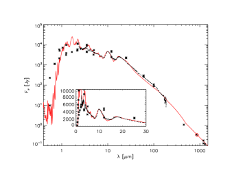
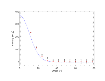
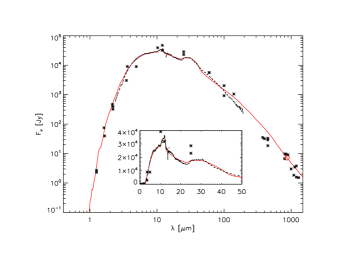
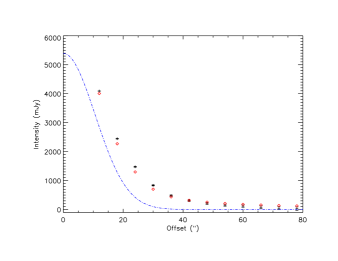
Figure 7: Left panel: best model (continuous red line) for ISO-SWS/LWS data of $o$ Cet (dashed black line) with photometric data (black stars). The red diamond is the LABoCa measurement at 870 $\mu$m. The inset shows the spectral range between 0 to 50 $\mu$m. Right panel: Differential aperture photometry on the LABoCa map of $o$ Cet (black symbols) compared to the synthetic brightness map derived from the best model (red symbols). The dashed blue line is the HPBW.

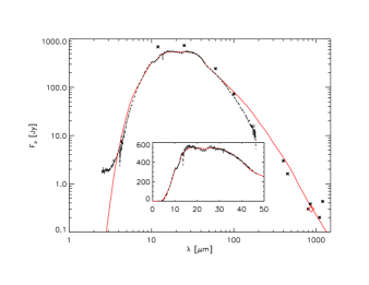
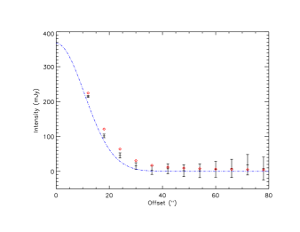
Figure 8: As Figure 9 for CW Leo.

Figure 9: As Figure 9 for AFGL 3068

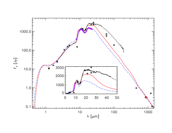
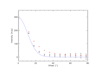
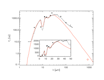
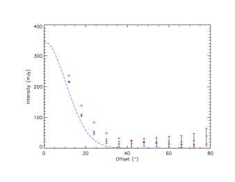
Figure 13: Left panel: IRC +10420 ISO-SWS/LWS spectrum (dashed black line) with the best model (continuous red line) together with the LRS spectrum (purple crosses) with its respective best model (dash-dot blue line). The black stars are the photometric data and the red diamonds the LABoCa measurement at 870 $\mu$m. The inset shows the spectral range between 0 to 50 $\mu$m. Right panel: Differential aperture photometry on the LABoCa map of IRC 10420 (black symbols) compared to the synthetic brightness map derived from the best model (red symbols). The dashed blue line is the HPBW.

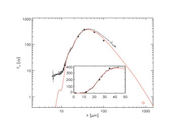
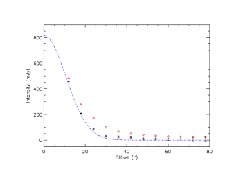
Figure 14: As Figure 9 for AFGL 5379.

Figure 15: As Figure 9 for IRAS 16342$-$3814.

The derived total flux at 870$\mu$m is included in the SED modelling and is in fair agreement with previous sub-millimetre observations given the intrinsic variability of some of the stars (see Fig. 9 to Fig. 15 in the appendix).

Table 1: Measured flux at 870 $\mu$m.

IRAS name	Alternative ID	Spectra type	Variability	Flux at 870 $\mu$m	Errora	rms	Ideal apertureb
				[mJy]	[mJy]	[mJy/pixel]	[″]
01037$+$1219	WX Psc	M9	LPV	145	3	0.38	42
02168$-$0312	$o$ Cet	M7	Mira	339	3	0.51	40
07209$-$2540	VY CMa	M3/M4II		1304	15	2.98	35
09452$+$1330	CW Leo	C		7243	9	1.98	48
16342$-$3814		PAGB		602	3	0.56	37
17411$-$3154	AFGL 5379	OH/IR		304	4	0.64	39
19244$+$1115	IRC $+$10420	F8Ia		243	3	0.46	38
22196$-$4612	$\pi$ Gru	S	SRb	143	3	0.38	42
23166$+$1655	AFGL 3068	C	Mira	299	5	0.85	38

4 The extended emission

To investigate the presence of any extended emission at 870 $\mu$m, we adjusted an elliptical Gaussian to the surface brightness map of each target with a free orientation of the axes of the ellipse (relevant in the case of asymmetric sources). The FWHM of the ellipse in both directions is compared to the FWHM of the theoretical beam. A source is considered extended if the difference in size between the source and the theoretical beam combining the errors is larger than a factor 3 in at least one direction (see parameter $s$ in Table 2). A position angle is derived for the resolved sources using a least square minimisation and is given in Table 2 (see parameter $PA$). We compute for the resolved sources both the major axis $a$ and the minor axis $b$ of the ellipse (see Table 2) and use the new values to investigate the extended emission.

From Table 2, extended emission at 870 $\mu$m is seen only for CW Leo and $\pi$ Gru in both directions and WX Psc and $o$ Cet in one direction.

Young et al. (1993) detected an extended emission at 60$\mu$m for CW Leo, $\pi$ Gru and $o$ Cet but did not observe any extended emission for VY CMa, AFGL 3068, IRC +10420, WX Psc and AFGL 5379.

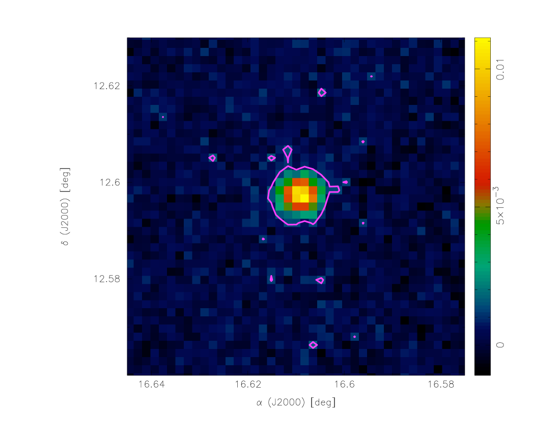
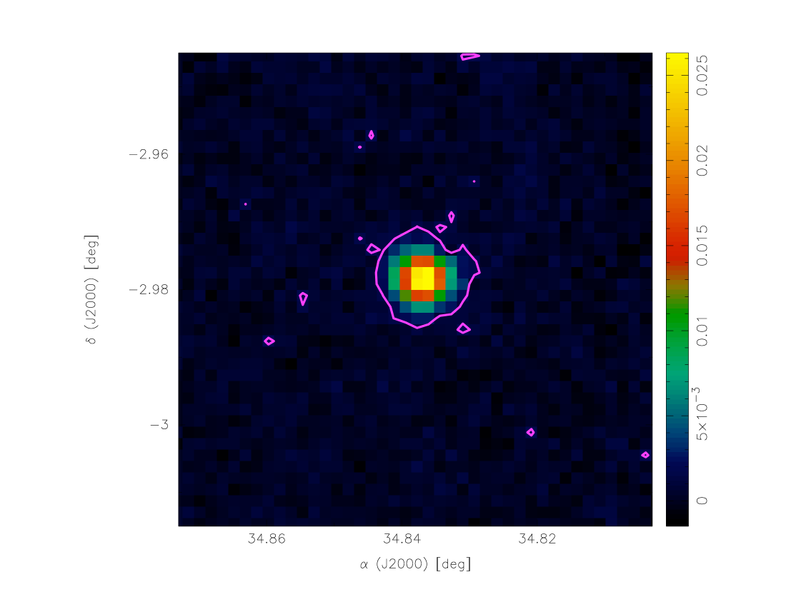
Figure 5: LABoCa brightness map for WX Psc in Jy (250″$\times$250″). The contour is drawn at a 3$\sigma$ level above the noise (1.3 MJy/sr).

Figure 6: LABoCa brightness map for $o$ Cet in Jy (250″$\times$250″). The contour is drawn at a 3$\sigma$ level above the noise (1.8 MJy/sr).

A 250″ $\times$ 250″ cut of the LABoCa maps for the resolved sources can be seen from Fig. 4 to Fig. 6. A 3$\sigma$ level above the noise contour is drawn. The FWHM of the adjusted ellipse in both $x$ and $y$ directions can be found in Table 2.

The four sources for which extended emission is found at 870 $\mu$m will be discussed in the following subsections.

4.1 CW Leo

CW Leo shows the largest extended emission of our set with a 25″ FWHM spherically symmetric CSE at 870 $\mu$m (see Fig. 4 and Table 2). This is not surprising, as this nearby carbon star is subject to a high mass loss rate and is surrounded by a thick CSE. The circumstellar shell has been imaged at different wavelengths, in the visible by Mauron and Huggins (2000), in the NIR by Leão et al. (2006), at 1.3 mm by Groenewegen et al. (1997b) and using CO lines by Huggins et al. (1998) and Fong et al. (2004).

CW Leo is known for being variable in the K band with a magnitude variation from 1.9 to 2.9 mag and in the M band with a variability $\sim$ 0.6 mag, the estimated period is $\sim$ 638 days (Dyck et al. 1991). It is also variable at radio-wavelengths (1.3 cm) with a 25% flux variation with a period of 535$\pm$52 days (Menten et al. 2006). This implies that CW Leo probably has variability at 870 $\mu$m. Despite the brightness of CW Leo, the variability and the extended emission at the LABoCa wavelength makes it unsuitable as a flux calibrator.

4.2 $\pi$ Gru

The 2D Gaussian fit of the LABoCa map of $\pi$ Gru shows an extended emission with a FWHM of 23.3″ following the east-west direction and 22″ following the north-south direction (see Fig. 4 and Table 2). Beyond the FWHM, $\pi$ Gru appears even more elliptical in the LABoCa map with a structure of about 60″ by 40″.

An asymmetry in the CO line profiles of this star has been observed by Sahai (1992) and by Knapp et al. (1999) with two velocity components being derived. A fast outflow with a speed greater than 38 km$s^{-1}$ and perhaps as high as 90 kms^-1 and a ”normal” outflow with a speed of about 11 kms^-1. Sahai (1992) suggested that the asymmetry in the line profiles is the result of a fast bipolar outflow collimated by an equatorial disk (major axis direction east-west). Knapp et al. (1999) proposed a model with a disk to explain the observed CO line profiles. In their model, the disk is tilted by 55^∘ to the line of sight with a major axis lying east-west. The asymmetry in the CO line profiles would then be related to the northern and southern halves of the disk, the fast outflow was not included in the modelling.

According to Huggins (2007), the creation of a disk/jet structure in AGB stars needs a binary system. In fact, $\pi$ Gru is the primary of a wide binary system with a G0V star as secondary (Proust et al. 1981; Ake & Johnston 1992). The large separation (of about 2.71″) makes it difficult for the companion to be responsible for the bipolar outflow. One possible explanation given by Chiu et al. (2006) is the presence of a much closer companion that has escaped detection and which would be the source of the high-velocity outflow. This possibility is supported by Makarov & Kaplan (2005) and Frankowski et al. (2007) who found significant discrepancies between Hipparcos and Tycho-2 proper motions of the star which indicates additional orbital motion with an orbital period shorter than the 6000 years derived by Knapp et al. (1999).

Sacuto et al. (2008) attempted to resolve the disk using MIDI/VLTI interferometric data at 10$\mu$m but the data were not conclusive. They do detect the presence of an optically thin CSE but it does not depart from a spherical shape. Sacuto et al. (2008) argue that the disk can be confused for a spherical shell if the system opening angle is larger than the interferometric angular coverage (60^∘). A poor $uv$ coverage can also be a reason for not resolving the disk.

If we assume that the extended emission observed in the LABoCa map is from the disk, geometrical constraints and the derived major and minor axes would imply a disk tilted by about 70^∘ to the line of sight with a major axis lying east-west, in agreement with Knapp et al. (1999). This higher angle could also explain why it is easy to confuse the disk for a spherical CSE.

4.3 WX Psc

WX Psc is an O-rich star known for being variable at infrared wavelengths with a magnitude variation from 1.29 magnitude in the M-band up to 2.83 magnitudes in the J-band, with a period of 660 days (Le Bertre 1993), $\Delta m=$1.5 at 10$\mu$m (Harvey et al. 1974) and $\Delta m=$1.2 at 18 cm (Herman & Habing 1985).

The LABoCa data show an extended emission of 23.6″ following one direction with a position angle of 84^∘ (see Fig. 6 and Table 2).

From previous CO interferometric observations, Neri et al. (1998) suggest that the star has two CSE components, a spherically symmetric component with a radius of 29.6″ and an elliptical component with a major axis of 9.8″ and a minor axis of 6.8″ with a position angle of $-$45^∘.

Hofmann et al. (2001) conducted interferometric observations of WX Psc in the J-, H- and K-bands. In the J-band, the results show a clear elongation along a symmetry axis with a position angle of $-$28^∘. This asymmetric structure is composed of two components, a compact elliptical core with a major axis of 154 mas and a minor axis of 123 mas and a fainter ”fan” shape structure with the opening angle of the fan from $-$8^∘ to $-$48^∘, out to distances of $\sim$200 mas. This ”fan” like structure is hardly seen in the H and the K band, where the dust shell displays a spherical symmetry. The J-band structure has been modelled by Vinković et al. (2004) who could reproduce the same structure by constructing a 2D radiative transfer model considering a bipolar jet which would sweep up material in the slower spherical wind and create a cone as seen in the NIR data. Inomata (2007) claimed the existence of such a bipolar outflow after analysing H₂O maser spectra of WX Psc and deriving a structure position angle in agreement with what found by Hofmann et al. (2001).

A V-band image of WX Psc, obtained with the VLT by Mauron & Huggins (2006), shows a spherically symmetric shell out to $\sim$50″ distance while in an HST-ACS image at 816 nm a highly asymmetric core is seen with an extension out to $\sim$ 0.4″ with a $-$45^∘ position angle. Mauron & Huggins conclude that WX Psc is similar to CW Leo in respect to the presence of a circular symmetry at large scale together with a strong asymmetry close to the star.

The asymmetric extended emission observed in the LABoCa map of WX Psc disagrees with Mauron & Huggins (2006) assumption by showing that the asymmetry in the dust structure can still be observed at bigger scales (up to 40″). This asymmetric dust structure is also in disagreement with the spherical gas envelope observed at 1.3 mm by Neri et al. (1998). This could be the result of an extremely complex mass-loss history with sudden changes in the mass loss rate during the life span of the star resulting in multiple shells with different geometries.

4.4 $o$ Cet

Also known as Mira, it is the prototype for Mira-type variables. It is also one of the closest O-rich AGB stars with an estimated distance of 131$\pm$18 pc (Perryman et al. 1997). Its variability reaches 3 magnitudes in the V-band with a period of 331 days (GCVS).

The LABoCa map shows an asymmetric CSE with an elongated core of 22.8″ with a position angle of 79^∘ (see Fig. 6 and Table 2).

From previous studies, we know that Mira shows asymmetry on all scales. At large scale a turbulent wake 2^∘ long was observed in emission in the ultraviolet (Martin et al. 2007) and in the 21 cm HI line (Matthews et al. 2008). At small scale the star itself is asymmetric (Karovska et al. 1997).

The data of Josselin et al. (2000) show an asymmetric ”peanut” like molecular envelope lying roughly east-west with two ”holes” located at about 4″ north and south with three velocity components which suggest the presence of a bipolar outflow. Unlike $\pi$ Gru however, the bipolar outflow velocity is low and close to the velocity of the spherical component which is about 8 kms^-1 and as such cannot account for the observed asymmetry. In order to explain the unusual shape of Mira, Josselin et al. (2000) suggest that the departure from sphericity occurs very early on the AGB, if not since the beginning. Furthermore, the bipolar outflow could accelerate as the star evolves along the AGB phase.

Like $\pi$ Gru, $o$ Cet is part of a binary system (Joy 1926; Karovska & Nisenson 1993) with a close companion at a distance of 0.61″$\pm$0.03″ and a position angle of 111^∘. The companion is expected to be a relatively hot star (a main sequence star or a white dwarf) (Karovska & Nisenson 1993).

Using Spitzer data, Ueta (2008) shows the presence of an astropause (a stellar analogue of the heliopause) at 160 $\mu$m with a slightly extended core at a position angle of 70^∘ and derives a correlation between the dust emission at 160 $\mu$m and the turbulent wake observed in the ultraviolet. The position angle of 79^∘ that we find at 870$\mu m$ is close to the 70^∘ position angle found by Ueta (2008) at 160$\mu m$ and implies that the extended ellipsoid lies east-west, which is also in agreement with the findings of Josselin et al. (2000).

Table 2: Results of the 2D elliptic Gaussian fit.

IRAS name	Alternative ID	FWHMx	FWHMy	$PA$	$a$	$b$	$s_{x}$	$s_{y}$
		[″]	[″]	[∘]	[″]	[″]
01037$+$1219	WX Psc	23.6$\pm$0.4	21.7$\pm$0.4	84	23.6	21.7	4.2	2.5
02168$-$0312	$o$ Cet	22.7$\pm$0.2	21.4$\pm$0.2	79	22.8	21.4	3.6	2.4
07209$-$2540	VY CMa	19.2$\pm$0.2	20.0$\pm$0.3				1.4	0.2
09452$+$1330	CW Leo	25.0$\pm$0.1	25.2$\pm$0.1				6.8	10.0
16342$-$3814		20.7$\pm$0.1	20.4$\pm$0.1				0.7	0.6
17411$-$3154	AFGL 5379	20.9$\pm$0.3	21.2$\pm$0.3				0.8	1.9
19244$+$1115	IRC $+$10420	22.0$\pm$0.2	20.9$\pm$0.2		22.0	20.9	2.5	1.5
22196$-$4612	$\pi$ Gru	23.1$\pm$0.4	22.2$\pm$0.4	-68	23.3	22.0	3.6	3.3
23166$+$1655	AFGL 3068	21.2$\pm$0.4	20.7$\pm$0.3				1.2	1.0
Uranus		20.4$\pm$0.7	20.3$\pm$0.5
PSF		20.2$\pm$0.7	20.1$\pm$0.5

5 SED Modelling and synthetic brightness maps

5.1 The radiative transfer code DUSTY

Theoretical spectral energy distributions (SEDs) were computed using the 1D radiative transfer code DUSTY (Ivezić et al. 1999).

Originally, DUSTY considers only spherical dust grains, but we added a subroutine to the main code to also be able to consider a Continuous Distribution of Ellipsoids (CDE) as the distribution of grain shapes. The ellipsoids are randomly oriented and have different shapes but have always the same volume. CDE has been very successful in reproducing the SED features of C-rich stars (e.g. Hony et al. 2002) and the observed features of silicates (e.g. Bouwman et al. 2001).

In Fig. 1 the difference in shape of the dust features (in this case SiC at 11$\mu$m and MgS around 30$\mu$m) when using a spherical grain distribution or CDE is shown. The ISO-SWS/LWS spectra of CW Leo is also plotted in order to compare the shape of the modelled features to the observed data. When using the CDE, the features are broader and are a better match to the observed data. Additionally, the position of the peaks are shifted compared to the spherical case and in better agreement with the observations.

One of the consequences in using the CDE is that for a same density distribution we obtain a much higher level of flux in the FIR than when using spherical grains (see Fig. 2). This leads to the use of steeper density distributions in order to fit the observed data in that wavelength range.

We adopted the CDE distribution for all the models. For a more detailed description of the CDE and for the scattering and absorption coefficient equations, see Min et al. (2003).

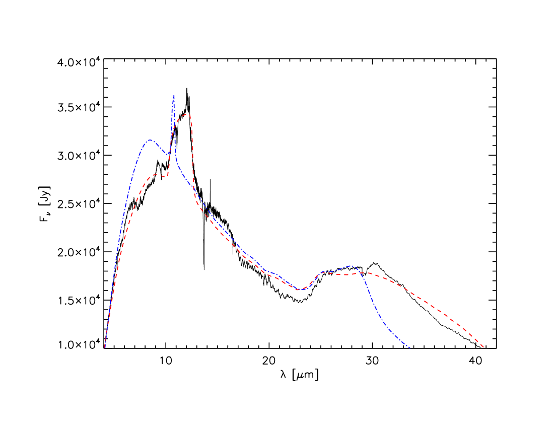
Figure 1: Comparison between the shape of the dust features of the best model for ISO-SWS data of CW Leo (black full line) using spherical grains (blue dash-dot line, 2% SiC, 4% MgS and 94% amorphous carbon) and using CDE (red dashed line, 12% SiC, 22% MgS and 66% amorphous carbon). The SiC feature is at 11$\mu$m and the MgS feature is around 30$\mu$m.

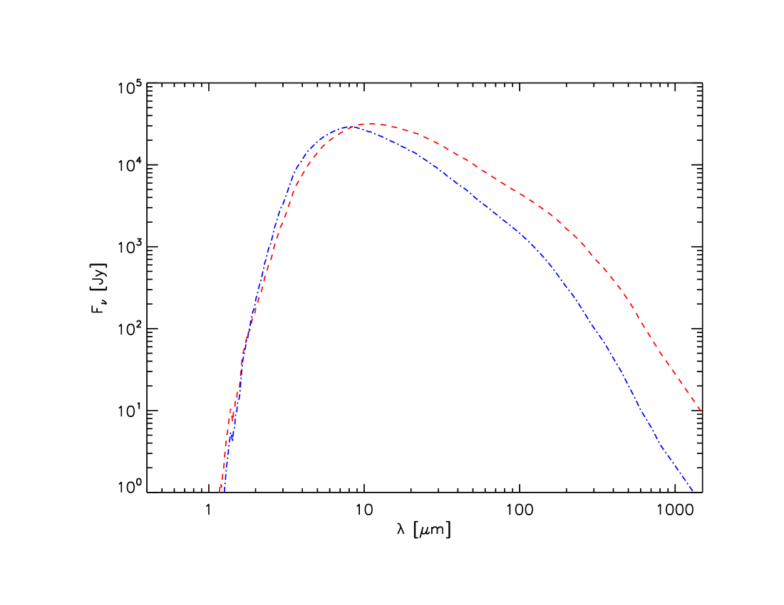
Figure 2: Comparison between spherical grains (blue dash-dot line, 100% amorphous carbon) and CDE (red dashed line, 100% amorphous carbon) for a same density distribution and optical depth.

5.2 The dust chemical composition

DUSTY comes with a built-in library of optical properties for six common dust components but it can also handle additional components if provided with the adequate optical properties.

For O-rich stars we used the recent MARCS stellar atmosphere models for cool stars (see Gustafsson et al. 2008) as a radiative source. The models cover a wavelength range from 0.2$\mu$m to 20$\mu$m. Beyond 20$\mu$m we used Rayleigh$-$Jeans approximation.

Concerning the dust composition, we investigated the following dust species:

- Amorphous silicate (Mg_xFe_2-xSiO₄): it is the dominant component in O-rich stars. Only by using amorphous silicate we can reproduce the overall shape of the SED. It is also responsible for the prominent 9.7 $\mu$m feature and the 18 $\mu$m feature. There are different sets of silicates which differ slightly in shape and in the position of the features. For this work we investigated three different types of silicates: Draine & Lee (1984), Ossenkopf et al. (1992) and Dorschner et al. (1995). In some cases Dorschner et al. (1995) grains give a better agreement with the observed silicate features where in some other cases Ossenkopf et al. (1992) grains are a better representation. Ossenkopf et al. (1992) grains are considered better suited for cool oxygen-rich dust which are representative in OH/IR stars (see Ossenkopf et al. 1992 for a discussion).

- Amorphous aluminium oxide (Al₂O₃): In the dust condensation sequence, it is considered as the first condensate. It was successfully used to reproduce the broad 12 $\mu$m feature in IRAS spectra of AGB stars (Onaka et al. 1989 ; Egan & Sloan 2001), UKIRT and ISO-SWS spectra (e.g., Speck et al. 2000 ; Maldoni et al. 2005 ; Blommaert et al. 2006). For this analysis we are using the grains optical properties by Begemann et al. (1997).

- Metallic iron (Fe): it was successfully used by Kemper et al. (2002) to correct the overestimated opacity in the near-infrared (NIR) for OH/IR stars.

For C-rich stars we used the synthetic models of Loidl et al. (2001) and investigated 3 carbon-rich dust species:

- Amorphous carbon (AmC here) : It is the main component in C-rich stars. Two different sets of amorphous carbon grains were tested ; Preibisch et al. (1993) and Rouleau & Martin (1991). The absorption coefficient of the two components is very similar in NIR and mid-infrared but becomes different in the far-infrared (FIR) where Rouleau & Martin (1991) grains give more flux. Using a CDE distribution, Preibisch et al. (1993) grains give a better fit to the data in the sub-millimetre range than Rouleau & Martin (1991). In the following, AmC will refer only to Preibisch et al. (1993) grains.

- Magnesium sulfide (Mg_0.9Fe_0.1S): It has been used by Hony & Bouwman (2004) to reproduce the 30 $\mu$m feature. In this work we use the optical properties of Preibisch et al. (1993).

- Silicon carbide (SiC): Two different types of silicon carbide were tested, Pégourié (1988) and Pitman et al. (2008) grains. The latter turned out to be a better candidate for modelling the 11 $\mu$m feature, regarding both shape and peak position. The peak position was especially an issue as Pégourié (1988) grains showed an important offset to the blue compared to the observed data. In the following sections we will only refer to the Pitman et al. (2008) grains.

5.3 Modelling

A grid of models was constructed by varying the following physical parameters : the effective temperature $T_{\rm eff}$ in the range of 2400 K to 3500 K), the dust condensation temperature $T_{\rm c}$ ranging from 500 K to 1200 K, the dust chemical composition, the optical depth $\mathbf{\tau}_{\lambda}$ at 0.55 $\mu$m and the density power index which was varied from $-$2.7 to $-$1.7. The maximum outer radius of the shell was set to be 10,000 times the inner shell radius and the dust grain volume when averaged by a sphere is equal to $4/3\pi a^{3}$ with $a$ set to 0.05 $\mu$m. More details about the construction of the grid of models can be found in Appendix C.

Comparisons between the models and the data were made using an automated fitting routine and the best fit was selected based on a least square minimisation technique. The models were compared to the ISO Short Wavelength Spectra (SWS), retrieved from Sloan et al. (2003) database, ISO Long Wavelength Spectra (LWS) spectra retrieved from ISO archives and when available, photometric data from the visible to the millimetre were retrieved from the literature (see Table 5 for references). The LWS spectrum was shifted to match the SWS flux level. SWS and LWS spectra were available for all the stars except for IRC +10420 for which we have only the SWS spectrum. The consistency of the flux calibration between the SED and the IRAS photometry was checked for all the stars. The ISO data of WX Psc shows a significant discrepancy compared to the IRAS flux, so we decided to recalibrate the SED to the IRAS photometry. The SED was corrected by a factor of 0.6. Hofmann et al. (2001) also suggest the recalibration of the ISO data of WX Psc to the IRAS photometry. The spectroscopic data and the photometry points were weighted by taking into account their respective spectral resolution. Since one of the main goals of this study is to compare the synthetic brightness maps at 870$\mu$m to LABoCa maps, we enhanced the weight of the LABoCa point compared to the other sub-millimetre measurements to ensure a good correspondence.

[c]

Table 3: SED fitting results.

O-rich stars
Name	$T_{\rm eff}$	$T_{\rm c}$	$\mathbf{\tau}_{\lambda}$	n	$D$	$V_{gas}$	$L$ (x104)	$\dot{M}$ (x10-6)	$M_{\rm d}$ (x10-5)	${M}$ (x10-3)	Am. Silicate	Alumina	Fe	$\dot{M}_{ref}$ (x10-6)
	[K]	[K]			[Kpc]	[Kms-1]	L☉	[M${}_{\sun}/yr$]	[M☉]	[M☉]	[%]	[%]	[%]	[M${}_{\sun}/yr$]
WX Psc	2500	1010	9	-2.0	0.75a	20b	1.1	13	17	36	98 Ossen.		02	0.3$-$8b
$o$ Cet	2600	1000	0.12	-1.9	0.128c	8b	1.4	0.11	0.11	0.11	100 Dorsch.			0.5k
VY CMa	2500	1100	13	-2.1	1.14r	47b	27.5	203	600	(…)	98 Ossen.		02	100n$-$300o
IRAS 16342$-$3814	2600	1000	480	-2.2	2i	46h	0.04	319	128	< 140	75 Ossen.		25	300i
AFGL 5379	2600	700	52	-2.3	1.19d	24b	0.5	46	97	< 250	97 Dorsch.		03	9$-$200q
IRC $+$10420 (ISO)	7000	750	5	-2.2	5e	42b	47	693	1980	< 4400	99.5 Dorsch.		0.5	700$-$900m
IRC $+$10420 (LRS)	7000	750	4	-2.2	5e	42b	39	260	522	< 1600	90 Dorsch.	08	02	700$-$900m
$\pi$ Gru	3000	900	0.04	-2.0	0.153c	11g	1.04	0.05	0.01	0.06	50 Ossen.	50		0.2$-$0.7l
C-rich stars
Name	$T_{\rm eff}$	$T_{\rm c}$	$\mathbf{\tau}_{\lambda}$	n	$D$	$V_{gas}$	$L$ (x104)	$\dot{M}$(x10-6)	$M_{\rm d}$ (x10-5)	${M}$ (x10-3)	Am. C	SiC	MgS	$\dot{M}_{ref}$(x10-6)
	[K]	[K]			[Kpc]	[Kms-1]	L☉	[M☉]	[M☉]	[M☉]	[%]	[%]	[%]	[M${}_{\sun}/yr$]
CW Leo	2650	1050	25	-2.3	0.135j	17f	0.9	7	1.2	6.2	66	12	22	22j
AFGL 3068	2650	1000	135	-2.5	1.05d	16f	1.4	110	3.6	< 300	78	04	18	20$-$62p

• References. (a) van Langevelde et al. (1990); (b) Kemper et al. (2003); (c) Hipparcos (Perryman & ESA 1997); (d) Yuasa et al. (1999); (e) Jones et al. (1993); (f) Groenewegen et al. (1996); (g) Knapp et al. (1999); (h) He et al. (2008); (i) Sahai et al. (1999); (j) Groenewegen et al. (1998b); (k) Loup et al. (1993); (l) Groenewegen et al. (1998a); (m) Dinh-V-Trung et al. (2009); (n) Jura & Kleinmann (1990); (o) Harwit et al. (2001); (p) Ramstedt et al. (2008); (q) Kastner (1992); (r) Choi et al. (2008).

5.3.1 SED fitting results

The modelling results are summarised in Table 3. Fig. 9 to Fig. 15 show the comparison between the models and the data. We can see that the synthetic models are in most cases in good agreement with the observed data despite the adopted assumption of spherical symmetry which is not valid for all the stars (see Section 4).

Concerning $\pi$ Gru, the discrepancy between the model and the real SED may be explained by the fact that the O-rich MARCS model used as radiative source is not adapted for S-stars. As the CSE is optically thin, the features seen in the synthetic model are mostly that of the MARCS model.

The model for IRC +10420 agrees poorly with the observations between 15$\mu$m and 100$\mu$m. The ISO-SWS spectrum shows a high flux level between 15$\mu$m and 45$\mu$m. This high level of flux could not be reproduced by our modelling (see Fig. 15). This ”jump” is not seen in the IRAS Low Resolution Spectrum (LRS) what suggests that the ”jump” may be an artefact of the SWS data reduction. Connecting together the different SWS segments can be difficult as each segment relies on the calibration of the previous one, this issue is discussed in Sloan et al. (2003). Previous analysis of IRC +10420 (e.g. Oudmaijer et al. 1996) used the LRS spectrum in the SED fitting of the star which we could easily model in Fig. 15.

In the case of the OH/IR star AFGL 5379, the FIR excess is not well reproduced by the modelling (see Fig. 15) despite the use of metallic iron which was suggested by Kemper et al. (2002) to correct the FIR excess of OH/IR stars.

From the output of DUSTY, it is deduced that the photospheric flux of the central source is negligible at 870$\mu$m in the case of most of our stars except for $o$ Cet and $\pi$ Gru for which the photospheric flux contributes up to 50% to the total flux observed at 870$\mu$m.

5.3.2 Density distribution

Contrary to previous analyses which used a density distribution following an $r^{-2}$ density power law or even shallower densities to match the observations (e.g. Sopka et al. 1985, Groenewegen 1997a ; Blanco et al. 1998 ; Lorenz-Martins et al. 2001 ; Gautschy-Loidl et al. 2004), our models follow a steeper density distribution ( $\propto r^{-2.3}$ for AFGL 5379 and CW Leo, $\propto r^{-2.5}$ for AFGL 3068) (see the density power index ”n” in Table 3).

The main difference between those analyses, with a shallow density distribution, and our analysis is that they used spherical grains distribution while we used CDE. Section 5.1 discusses what the CDE does to the shape of dust features compared to the spheres distribution. We clearly see in the spectral energy distribution in Fig. 1 that CDE gives more realistic shape and peak position of the dust features (see also Min et al. 2003) but at the same time CDE gives a higher level of flux in the sub-millimetre (see Fig. 2). This leads to the use of a steeper density distribution law than $r^{-2}$ in order to reproduce the observed data with the uncertainty on the density power being $\pm 0.05$.

5.3.3 Mass$-$loss

The derived physical parameters from the SED modelling can be used to constrain the mass-loss rate $\dot{M}$ of our sample of stars.

For a constant mass-loss rate and a constant dust velocity, the optical depth $\mathbf{\tau}_{\lambda}$ is related to the mass-loss rate via (Groenewegen et al. 1998b) :

$$\mathbf{\tau}_{\lambda}=5.405\times 10^{8}\frac{\dot{M}\ \Psi\ Q_{\lambda}/{a}}{r_{\rm c}\ R_{*}\ V_{\rm d}\ \rho_{\rm d}}$$ (2)

Where $\dot{M}$ is in M_☉/yr, $V_{\rm d}$ is the dust velocity in km s^-1 , $R_{*}$ is the stellar radius in solar radii, $r_{c}$ is the inner dust radius in stellar radii, $Q_{\lambda}$ is the absorption coefficient, $a$ is the dust grain radius in cm which in the case of CDE is the radius of a sphere with the same volume as the ellipsoid, $\Psi$ is the dust-to-gas mass ratio which we assumed to be 0.005 and $\rho_{\rm d}$ is the grain density in g cm^-3.

The parameters that are derived from the SED modelling are the optical depth at a specific wavelength $\mathbf{\tau}_{\lambda}$, $R_{*}$ and $r_{\rm c}$ which can be computed using the effective temperature $T_{\rm eff}$ and the dust condensation temperature $T_{\rm c}$ and by assuming a distance. The assumed distances are listed in Table 3 together with the references.

We assumed the dust velocity $V_{d}$ as being equal to the gas terminal velocity $V_{gas}$ and used expansion velocities derived from CO line measurements (see Table 3). From equation 2 we can see that a change on the dust velocity has a linear affect on the mass-loss rate.

The dust grain density for silicates varies from 2.8 g cm^-3 to 3.3 g cm^-3 (see Ossenkopf 1992). We assumed an average value of 3 g cm^-3 for all O-rich stars. Concerning C-rich stars, we adopted the density distribution of the amorphous carbon used in our modelling, which is 1.85 g cm^-3 (see Preibisch et al. 1993 and Bussoletti et al. 1987).

The mass absorption coefficient $\kappa_{\lambda}=\frac{3Q_{\lambda}}{4a\rho}$ follows directly from DUSTY outputs and ranges from $\kappa_{870\mu m}\sim$ 2 cm²g^-1 for M-stars and $\kappa_{870\mu m}\sim$ 35 cm²g^-1 for C-stars with intermediate values of 4 cm²g^-1 and 8 cm²g^-1 for the OH/IR star AFGL 5379 and the S-star $\pi$ Gru, respectively. For the post-AGB star IRAS 16342$-$3814, we find $\kappa_{870\mu m}\sim$ 20 cm²g^-1 because of the the presence of a high fraction of iron which has a high opacity. These results are a magnitude higher than what is predicted by Draine (1981) for grains in the interstellar medium. Sopka et al. (1985) claim an order of magnitude uncertainty on the parameter when considering circumstellar grains rather than interstellar.

The derived mass-loss rates are of the same order as the one estimated in previous studies (see Table 3). The difference is within the predicted uncertainty for $\dot{M}$ estimates. One should keep in mind the dependence of $\dot{M}$ on the distance which can be very uncertain for AGB stars and also the dependence on the gas-to-dust ratio which is very difficult to constrain and can highly vary from one star to another. Ramstedt et al. (2008) discuss the reliability of mass-loss rate estimates for AGB stars and compare $\dot{M}$ values from CO line measurements and from SED modelling. The agreement between the two methods is within a factor $\sim$3 which they consider as the minimal uncertainty in present mass-loss rate estimates.

By assuming a constant mass-loss and a constant dust velocity and by using the derived size of each source, we can estimate the total mass of the CSE for each star. The minimum diameter of the CSE is assumed to be 3 times the average FWHM after deconvolution from the beam. The derived total mass of the CSE $M$ is listed in Table 3. In the case of unresolved CSEs, the calculated total mass represents an upper limit as the size derived from the observations is overestimated.

5.3.4 Dust mass in CSEs

Using a simple approach, we can estimate the total dust mass in the envelope M_d, assuming the dust at 870${\mu}$m is optically thin, by (Hildebrand, 1983) :

$$M_{\rm d}=9.52\times 10^{36}\frac{F_{\lambda}D^{2}}{\kappa_{\lambda}B_{\lambda}(T_{\rm d})}$$ (3)

Where $F_{\lambda}$ is the observed LaBoCa flux in erg s^-1cm^-3 (corrected from photospheric contamination for $\pi$ Gru and $o$ Cet), D is the distance in pc, $\kappa_{\lambda}$ is the dust opacity in cm²g^-1 and $B_{\lambda}(T_{\rm d})$ is the Planck function at the temperature where the dust emission peaks in erg s^-1cm^-3. From the parameters in Table 3 and the DUSTY outputs, we can determine the total dust mass for each of our object. The main uncertainty here is the determination of the dust temperature, the distance and the mass absorption coefficient. However, this approach should give us an order-of-magnitude estimate of the dust mass (see M_d in Table 3) in the envelope.

5.4 Intensity brightness maps

Once a best spectral energy distribution (SED) model was selected for each star, we retrieved from DUSTY the intensity brightness profile at the LABoCa wavelength. Each 1D intensity profile was converted to the observed 2D pixel grid and was convolved with a 2D PSF of the size of the experimental HPBW. We then compared the synthetic brightness maps to the LABoCa maps.

For a better visualisation we used differential aperture photometry on the data. What we expect to see when doing that for a source with a symmetric and homogeneous non detached CSE is a gaussian profile with a FWHM wider than the one obtained for a point source and representative of the extended emission. The gaussian profile would be disrupted if there is asymmetry and/or if there is any extra structure around the star such as a disc.

The background variation is the main source of photometric errors in bolometric data. Any constant background would be subtracted with the differential aperture photometry but its variation can still be seen and would essentially affect the parts with a low signal (the wings of the profile) and increase the photometric error estimation.

The comparison between the LABoCa maps and the synthetic maps can be seen from Fig. 9 to Fig. 15. A good agreement is found between the synthetic map and the LABoCa map for $o$ Cet, CW Leo, AFGL 3068. For $\pi$ Gru, the synthetic brightness map is close to the LABoCa data up to 20$\arcsec$ but after that the intensity in the synthetic map drops quickly to zero while we still have flux ($\sim$10mJy) in the LABoCa map. This can be due to the asymmetry observed in the LABoca map (see Fig. 4) and which is not taken into account in the modelling. The synthetic brightness maps of IRC +10420, AFGL 5379 and IRAS 16342$-$3814 predict more flux than the LABoCa maps up to 50$\arcsec$. At larger distance, the models are within the error bars of the LABoCa data. For IRC +10420 and IRAS 16342$-$3814 (Dijkstra et al. 2003) departure from spherical symmetry may be the cause. WX Psc synthetic map shows an important discrepancy with the LABoCa map. The synthetic map predicts more flux than observed and a more extended structure around the star, although the SED is well fitted.

The degree of agreement between the synthetic brightness maps and the LABoCa maps does not seem to be related to the quality of the SED modelling. Note that this discrepancy is not related to the assumed distance ($D$). Both the luminosity ($L$) and the angular scale ($R$) depend in the same way on the adopted distance ($L/D^{2}=constant$, while $L\sim R^{2}$, so $R/D=constant$).

In most cases, the models predict more dust than what is seen in the observed data. We tested decreasing the maximum value of the CSE outer boundary, but that did not make any difference up to a certain value and after that the quality of the SED model became poor. This is not surprising, as the outer boundary set in DUSTY is a maximum limit for the calculation of the dust and does not represent the final size of the CSE. The only risk would be to under estimate the limit, but that was not our case.

The main limitation in the modelling is the spherical symmetry assumption. While it does not stop us from obtaining a decent fit to the SEDs even for the asymmetric sources it clearly shows its limitation when deriving synthetic intensity profiles. It is probably the reason we find a poor agreement between the synthetic brightness maps and the LABoCA intensity profiles. This clearly shows that we cannot rely only on SED modelling to properly constrain the physical parameters of CSEs. Combining both modelling of the SED and the intensity profile would be the ideal.

SABoCa data have been collected for WX Psc and $o$ Cet and still need to be analysed. SABoCa is an APEX bolometer operating at 350$\mu$m with an expected sensitivity 5 times better than LABoCa. These new data will have a better spatial resolution than the LABoCa data and should improve the results of this paper for these two stars.

6 Conclusion

This paper presents the first LABoCa observations of evolved stars. We show in this study that it is possible to resolve the extended emission around AGB stars at 870 $\mu$m.

Extended emission has been found for CW Leo, $\pi$ Gru, WX Psc and $o$ Cet, with an asymmetric structure around $\pi$ Gru, WX Psc and $o$ Cet.

Using SED modelling results, the mass-loss rate has been derived for all the stars with a reasonable agreement with previous literature data and the total mass-loss has been estimated as well as the dust mass.

The SEDs and intensity profiles have been modelled with a 1D radiative transfer code. In most cases it is difficult to fit both constraints simultaneously. For some stars, departures from spherical symmetry are known from other observations at different wavelengths and different spatial scales. The asymmetry may be the reason why it is not possible to fit both SEDs and intensity brightness maps in a consistent way given that we assumed spherical symmetry in the modelling. The current single dish observations still lack the spatial resolution to really probe the dust structure at 870 $\mu$m.

Appendix A LABoCa maps

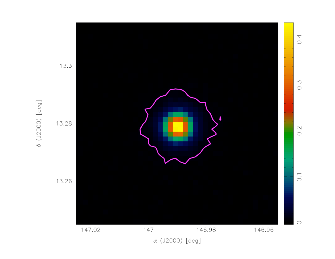
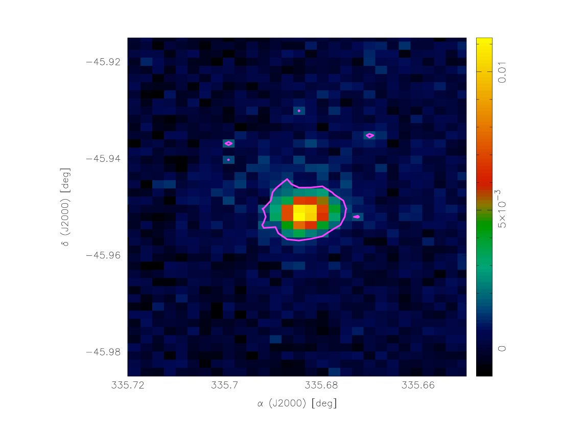
Figure 3: LABoCa brightness map for CW Leo in Jy (250″$\times$250″). The contour is drawn at a 3$\sigma$ level above the noise (7 MJy/sr).

Figure 4: LABoCa brightness map for $\pi$ Gru in Jy (250″$\times$250″). The contour is drawn at a 3$\sigma$ level above the noise (1.3 MJy/sr).

Appendix B Data reduction and calibration

B.1 Data reduction

The data reduction can be summarised as follows :

In a first step, the data are corrected for the atmospheric opacity using skydip scans. Thereafter, they are converted from the raw units to Jy flux units (see the next section concerning the flux calibration). After flat-fielding, correlated noise is removed by subtracting the median noise across the array. The data are then filtered based on a low- and high-frequency cut-off. The final map is weighted by the inverse of the variance and gridded to a 6″ pixel size.

Removing the correlated noise and filtering low frequencies are two very sensitive steps when looking for extended emission, because it is not possible to distinguish between a uniform extended emission and correlated noise observed by the bolometers. As a result, any uniform extended emission would be filtered out when performing the noise removal step. For this reason, we decided to use an iterative reduction technique developed by F. Schuller at the Max-Planck-Insitut für Radioastronomy (MPIfR) which is meant to save the extended emission if present. The technique was successfully used in a (sub)millimetre survey of the galactic plane (see Schuller et al. 2009).

To execute this technique, we first perform the data reduction following the reduction steps described above. At the end of this first reduction, we use the resultant map to flag and select all signal above a 3 $\sigma$ level. We then remove that part of the signal and we re-run the reduction procedure on the residual signal to enhance any faint emission left. At the end of this step, we put back the subtracted flux. This constitutes one iteration block. The iteration is repeated several times until a convergence in the signal-to-noise is obtained.

B.2 Calibration

BoA provides a flux calibration procedure which convert the maps from the raw units (Volts/beam) to Jy/beam. This procedure uses a Volt to Jy conversion factor specific to the instrument and a correction factor based on the ratio between the observed flux for a primary calibrator (a planet) and its predicted flux at the LABoCa frequency and beam and for a specific observing time. BoA uses the primary calibrators to calibrate a list of secondary calibrator stars. The calibration factor for a science star is obtained by interpolating between the two calibration factors of the two calibrators (primary or secondary) bracketing the science object in time. The calibration is done to the peak flux.

This calibration method is adapted to point sources but if used with extended sources, only a fraction of the total flux is enclosed within the beam which would lead to an overestimation of the flux. Therefor, we decided to develop our own reduction technique using only primary calibrators and by using aperture photometry. We chose to only use Uranus, Mars, Neptune and Venus observations as calibrators.

Using aperture photometry, we computed the integrated flux difference between two successive apertures in a map. This way, we take out any constant noise from the background. A 1D Gaussian is then fitted to the obtained profile.

The Astro software from the Gildas package provided us with the expected total flux for each planet at the LABoCa frequency and for the right observing date. The calibration factor is then the ratio between the expected total flux and the detected signal within an aperture of 3 sigma radius (corrected by the 99.73% factor).

Appendix C Grid of models

After studying the effect of the different input parameters on the synthetic SED, we first constructed a grid of over 47,000 models by varying the following physical parameters :

- The optical depth $\mathbf{\tau}_{\lambda}$ at 0.55$\mu$m : Studying the effect of varying the optical depth on the resultant SED, it appeared that a change of about 10% has a significant effect on the shape of the model. This means that a better sampling is needed at low optical depths than at high values. For this reason, we varied $\mathbf{\tau}_{\lambda}$ from 0.01 to 664 following a power law $\mathbf{\tau}_{\lambda}=0.01\times 1.4^{i}$ (were $i$ is the index) which gives a finer sampling at low values.

- The effective temperature $T_{\rm eff}$ was varied from 2400 K to 3500 K, which is a typical temperature range for AGB stars, with a step size of 200 K. For IRC$+$10420 which is an F star, effective temperatures of 6000 K, 7000 K and 8000 K were tested.

- The dust condensation temperature $T_{\rm c}$ which determines the inner dust radius was varied from 500 K to 1200 K with a step size of 100 K.

- The dust chemical composition :
$\bullet$ For O-rich stars :
- Iron ranging from 0% to 30% with a step size of 10%.
- Alumina ranging from 0% to 60% with a step size of 20%.
- Amorphous silicates = 100%$-$Iron$-$Alumina.
$\bullet$ For C-rich stars :
- SiC ranging from 0% to 15% with a step size of 5%.
- MgS ranging from 0% to 30% with a step size of 10%.
- Amorphous carbon = 100%$-$SiC$-$MgS.

The dust grain size was set to 0.05$\mu$m, the maximum outer radius of the shell was set to be 10,000 times the inner shell radius and the density distribution was taken $\propto r^{-2}$.

We compared each star to the models using a least square minimisation routine and a first solution was derived for each star. From this result we constructed a second grid of models with a more refined sampling of the physical parameters : 100 K for $T_{\rm eff}$, 50 K for $T_{\rm c}$, 1% for Alumina, SiC and MgS and 0.5% for Iron, the optical depth was varied with steps of about 10% around $\mathbf{\tau}_{\lambda}$ of the first solution. This time the density distribution slope was also varied in order to match the observations, the power density index range was taken from -2.7 to -1.7 with a step size of 0.1. The observations were again compared to this second grid of models and a final solution was derived for each source (see Table 3).

Appendix D Tables

Table 4: List of observations.

IRAS name	Alternative ID	Observing date	Number of scans	Total integration time [s]
01037$+$1219	WX Psc	28-07-2007	3	105
		01-08-2007	6	210
		02-08-2007	10	350
		07-08-2008	9	315
		12-08-2008	2	70
		14-08-2008	9	315
		15-08-2008	6	210
			45	1575
02168$-$0312	$o$ Cet	28-07-2007	7	245
		02-06-2008	9	315
		03-06-2008	16	560
		04-06-2008	3	105
		15-08-2008	4	140
			39	1365
07209$-$2540	VY CMa	25-02-2008	4	125
		26-02-2008	2	70
		27-02-2008	1	35
			7	230
09452$+$1330	CW Leo	24-02-2008	2	70
		25-02-2008	4	125
		26-02-2008	9	300
		27-02-2008	18	528
		28-02-2008	5	145
		29-02-2008	3	105
			41	1270
16342$-$3814	$-$	28-07-2007	8	280
		15-08-2008	6	210
		16-08-2008	16	560
			30	1050
17411$-$3154	AFGL 5379	28-07-2007	8	280
		15-08-2008	9	315
		16-08-2008	4	140
			21	735
19244$+$1115	IRC $+$10420	28-07-2007	7	245
		13-08-2008	4	140
		14-08-2008	23	805
			34	1190
22196$-$4612	$\pi$ Gru	28-07-2007	4	140
		01-08-2007	5	175
		10-08-2008	18	630
		11-08-2008	10	350
		15-08-2008	2	70
			39	1365
23166$+$1655	AFGL 3068	28-07-2007	8	280

Table 5: Photometric data.

Star	$\lambda$	$F_{\nu}$	$reference$	Star	$\lambda$	$F_{\nu}$	$reference$	Star	$\lambda$	$F_{\nu}$	$reference$
	[$\mu m$]	[Jy]			[$\mu m$]	[Jy]			[$\mu m$]	[Jy]
$o$ Cet	0.55	229.94	( 1 )	CW Leo	1.25	2.3	( 21 )	WX Psc	1.23	3.17	( 1 )
	0.55	9.76	( 9 )		1.25	2.7	( 2 )		1.25	1.69	( 2 )
	0.7	1104.27	( 10 )		1.65	74.9	( 2 )		1.65	14.25	( 2 )
	0.7	1138.92	( 1 )		1.65	39.6	( 21 )		2.17	86.52	( 2 )
	0.88	2131.97	( 1 )		2.17	469	( 2 )		2.2	113.8	( 1 )
	0.88	5871.93	( 1 )		2.2	388.8	( 21 )		3.5	220	( 3 )
	0.9	5027.64	( 10 )		2.2	321.9	( 3 )		3.5	330.67	( 1 )
	1.04	7193.59	( 10 )		3.5	3046.1	( 3 )		4.9	365.1	( 3 )
	1.25	3128.15	( 2 )		3.6	9072	( 21 )		12	1120	( 4 )
	1.25	9698.38	( 10 )		4.9	9010.7	( 3 )		12	646.9	( 3 )
	1.25	3845.33	( 1 )		10.2	39188.4	( 21 )		25	929.3	( 3 )
	1.25	9748.4	( 1 )		12	47500	( 6 )		25	921	( 4 )
	1.65	4364.15	( 2 )		12	31773.4	( 3 )		34.6	498.5	( 5 )
	2.17	5118.35	( 2 )		25	23100	( 6 )		60	212	( 4 )
	2.2	11275.24	( 1 )		25	28610.8	( 3 )		60	175.3	( 3 )
	2.2	5446.6	( 1 )		60	5650	( 6 )		100	68.8	( 3 )
	2.2	5927.1	( 3 )		60	5585	( 3 )		100	67.5	( 4 )
	2.25	11149.2	( 10 )		100	2017.5	( 3 )		400	3	( 14 )
	3.5	4334.9	( 3 )		100	922	( 6 )		1200	0.16	( 19 )
	3.5	10023.4	( 10 )		140	1051.5	( 3 )		1200	0.33	( 19 )
	3.5	4606.73	( 1 )		377	35.2	( 22 )		1300	0.08	( 13 )
	4.9	3220.5	( 3 )		400	32	( 14 )
	5	5425.61	( 1 )		450	18.45	( 12 )	$\pi$ Gru	0.55	8.5	( 1 )
	12	2415.6	( 3 )		450	29	( 14 )		0.55	10.22	( 9 )
	12	4880	( 6 )		450	33.2	( 16 )		0.7	157.21	( 1 )
	25	2322.8	( 3 )		800	6.66	( 16 )		0.88	1602.43	( 1 )
	25	2260	( 6 )		811	9.8	( 22 )		1.25	3079.56	( 2 )
	60	301	( 6 )		850	9.45	( 12 )		1.25	2943.97	( 1 )
	60	263.2	( 3 )		900	9	( 14 )		1.65	5795.62	( 2 )
	100	108.9	( 3 )		1000	4	( 17 )		2.17	5812.06	( 2 )
	100	88.4	( 6 )		1100	1.85	( 16 )		2.2	4657.21	( 1 )
	450	1.09	( 12 )		1100	3.5	( 16 )		2.2	4552.7	( 3 )
	850	0.35	( 12 )		1136	3.5	( 22 )		3.5	2952.2	( 3 )
	1200	0.13	( 11 )		1200	1.58	( 11 )		4.9	1323.7	( 3 )
	1200	0.18	( 19 )		1200	3.8	( 19 )		12	908	( 6 )
	1300	0.12	( 13 )		1300	1.52	( 18 )		12	729.6	( 3 )
									25	437	( 6 )
VY CMa	0.55	2.1	( 9 )	IRAS 16342$-$3814	1.25	0.04	( 2 )		25	506.2	( 3 )
	0.7	27.74	( 10 )		1.65	0.06	( 2 )		60	77.3	( 6 )
	1.25	118.6	( 2 )		2.17	0.1	( 2 )		60	86	( 3 )
	1.65	239.8	( 2 )		12	16.2	( 6 )		100	23.3	( 6 )
	2.17	510	( 2 )		25	200	( 6 )		100	40.9	( 3 )
	4.9	3042.78	( 10 )		34.6	365.6	( 5 )
	12	9920	( 6 )		60	290	( 6 )	AFGL 3068	2.17	0.04	( 2 )
	12	9278.1	( 3 )		100	139	( 6 )		12	690	( 4 )
	25	6650	( 6 )						25	736	( 4 )
	25	12345.5	( 3 )	IRC $+$10420	1.23	10.94	( 8 )		60	244	( 4 )
	34.6	4387.5	( 5 )		1.25	10.38	( 2 )		100	72.7	( 4 )
	60	1450	( 6 )		1.65	15.58	( 2 )		400	3	( 14 )
	60	2318.4	( 3 )		2.15	25.52	( 8 )		450	1.61	( 12 )
	100	331	( 6 )		2.17	23.94	( 2 )		800	0.3	( 15 )
	100	2084.5	( 3 )		3.5	104.1	( 3 )		850	0.38	( 12 )
	400	10	( 14 )		4.35	152.1	( 7 )		1100	0.2	( 15 )
	450	9.5	( 12 )		4.9	179.2	( 3 )		1200	0.43	( 19 )
	800	2.81	( 16 )		8.28	148.7	( 7 )
	780	1.99	( 20 )		12	1280.8	( 3 )	AFGL 5379	1.25	0.01	( 2 )
	780	2.66	( 20 )		12	1350	( 6 )		1.65	0.02	( 2 )
	850	2.18	( 20 )		12.13	1292	( 7 )		2.17	0.04	( 2 )
	850	1.77	( 12 )		14.65	1263	( 7 )		4.35	158.5	( 7 )
	1100	0.79	( 20 )		21.34	2221	( 7 )		8.28	173.8	( 7 )
	1100	0.92	( 20 )		25	2911.5	( 3 )		12	1260	( 4 )
	1100	0.83	( 16 )		25	2310	( 6 )		12.13	1318	( 7 )
	1200	0.34	( 11 )		60	718	( 6 )		14.65	1204	( 7 )
	1200	0.69	( 19 )		60	566.9	( 3 )		21.34	1679	( 7 )
	1250	0.79	( 20 )		100	186	( 6 )		25	2720	( 4 )
	1250	0.58	( 20 )		450	0.95	( 12 )		60	1360	( 4 )
	1300	0.38	( 13 )		850	0.31	( 12 )		100	406	( 4 )
	1840	0.42	( 20 )		1200	0.5	( 19 )
	1840	0.27	( 20 )		1300	0.1	( 13 )

• References. (1) UBVRIJKLMNH Photoelectric Catalogue (Morel+ 1978); (2) 2Mass All-Sky catalogue (Cutri+ 2003); (3) COBE DIRBE point source catalogue (Smith+ 2004); (4) IRAS faint source catalogue, version 2.0 (Moshir+ 1989); (5) The 35um absorption line towards 1612MHz masers (He+ 2005); (6) IRAS catalogue of point sources, version 2.0 (IPAC 1986); (7) MSX6C Infrared point source catalogue (Egan+ 2003); (8) DENIS photometry of bright southern stars (Kimeswenger+ 2004); (9) The Hipparcos and Tycho catalogues (ESA 1997); (10) Catalogue of late type stars with maser emission (Engels 1979); (11) Radio emission from stars at 250GHz (Altenhoff+ 1994); (12) Submillimeter continuum SCUBA detections (Di Francesco+ 2008); (13) Walmsley et al. 1991; (14) Sopka et al. 1985; (15) Groenewegen et al. 1993; (16) Marshall et al. 1992; (17) Campbell et al. 1976; (18) Groenewegen et al. 1997; (19) Dehaes et al. 2007; (20) Knapp et al. 1993; (21) Le Bertre 1987; (22) Phillips et al. 1982.

Appendix E SED modelling

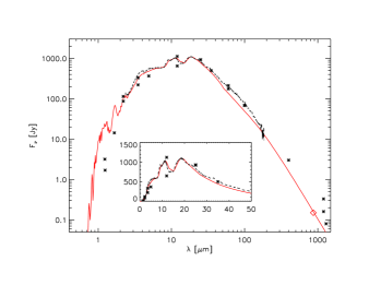
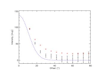
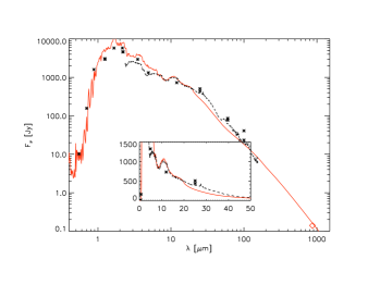
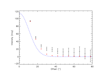
Figure 10: As Figure 9 for WX Psc.

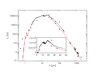
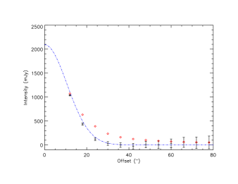
Figure 11: As Figure 9 for $\pi$ Gru.

Figure 12: As Figure 9 for VY CMa.