Autocorrelations in the totally asymmetric simple exclusion process and Nagel-Schreckenberg model

Abstract

We study via Monte Carlo simulation the dynamics of the Nagel-Schreckenberg model on a finite system of length $L$ with open boundary conditions and parallel updates. We find numerically that in both the high and low density regimes the autocorrelation function of the system density behaves like $1-|t|/\tau$ with a finite support $[-\tau,\tau]$. This is in contrast to the usual exponential decay typical of equilibrium systems. Furthermore, our results suggest that in fact $\tau=L/c$, and in the special case of maximum velocity $v_{\rm max}=1$ (corresponding to the totally asymmetric simple exclusion process) we can identify the exact dependence of $c$ on the input, output and hopping rates. We also emphasize that the parameter $\tau$ corresponds to the integrated autocorrelation time, which plays a fundamental role in quantifying the statistical errors in Monte Carlo simulations of these models.

I Introduction

The totally asymmetric simple exclusion process (TASEP) Spitzer (1970) is a simple transport model, of fundamental importance in nonequilibrium statistical mechanics. In addition to its mathematical richness, it has applications ranging from molecular biology to freeway traffic.

A TASEP consists of a chain of length $L$, with each site being either occupied by a particle or not, on which particles hop from left to right. See Fig. 1. If site $i=1$ is vacant a particle will enter the system with probability $\alpha$. If site $i=L$ is occupied the particle will leave the system with probability $\beta$. In the bulk of the system, a particle on site $i$ will hop to site $i+1$ with probably $1-p$ provided $i+1$ is vacant, otherwise it remains at site $i$.

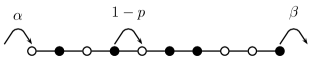
Figure 1: A TASEP with $L=10$.

TASEPs exhibit boundary-induced phase transitions, governed by the parameters $\alpha$, $\beta$ and $p$. In general, for a given $p$, there exist three possible phases, depending on $\alpha$ and $\beta$: a low-density phase, a high-density phase, and a maximum-current (or maximum-flow) phase.

In the context of traffic models, it is most appropriate to update all sites in parallel at each time-step. The stationary distribution of the TASEP with fully-parallel updates de Gier and Nienhuis (1999); Evans et al. (1999) is known exactly. (For reviews of the stationary properties of TASEPs with random sequential updates see Derrida (1998); Schütz (2001).) The Nagel-Schreckenberg (NaSch) model Nagel and Schreckenberg (1992) is an important generalization of the parallel-update TASEP, in which particles can move up to $v_{\max}\in\mathbb{N}$ sites per time step. The NaSch model is generally considered to be the minimal model for traffic on freeways Chowdhury et al. (2000). While many results are known rigorously for the TASEP, our understanding of the NaSch model and its further generalizations typically rely on numerical simulation. This is particularly true of traffic network models, in which the NaSch model is often a component (see for example Esser and Schreckenberg (1997); Schreckenberg et al. (2001); Cetin et al. (2002)).

In the current article we focus on dynamic (auto)correlation functions. The autocorrelations of the TASEP with random sequential update have been studied in P. Pierobon, A. Parmeggiani, F. von Oppen, E. Frey (2005); Adams et al. (2007) and display a separation of time scales between relaxation of local density fluctuations and collective domain wall motion. In particular, it was recently observed Adams et al. (2007) that the TASEP with random sequential update exhibits non-trivial oscillations in the power spectrum of the system density, in the low and high density phases. In this article, we further elucidate the nature of these non-trivial oscillations, and demonstrate that they extend to the NaSch model generally. We emphasize that all the simulations performed in this work used fully-parallel updates, including our simulations of TASEP (which we view as the special case of the NaSch model with $v_{\max}=1$).

I.1 Density autocorrelations

The system density, $n$, which is simply the fraction of sites which are occupied, is an important quantity in many applications, including traffic modeling. The relationship between density and flow is known as the fundamental diagram in the traffic engineering literature. While the stationary-state expectation $\langle n\rangle$ of $n$ is well understood for the NaSch model, and in fact known rigorously for the TASEP, the dynamic behavior of $n_{t}$ is non-trivial. In this article we numerically study the autocorrelation function $\rho_{n}(t):=(\langle n_{0}n_{t}\rangle-\langle n\rangle^{2})/\text{var}(n)$ of the general NaSch model, and find a very simple form for its finite-size scaling. Up to very small corrections, our simulations show that in both the high and low density phases we simply have

$$\rho_{n}(t)=\begin{cases}1-|t|/\tau,&|t|\leq\tau,\\ 0,&|t|\geq\tau,\\ \end{cases}$$ (1)

for some constant $\tau\propto L$.

The linear decay in (1) is in sharp contrast to the usual exponential decay typical of equilibrium systems. In fact, as discussed in section II.2, there are good theoretical reasons to believe that $\rho_{n}(t)$ must ultimately decay exponentially on sufficiently long time scales, rather than exhibit the strictly finite support suggested by (1). However, as demonstrated by the simulations in sections III and IV, any corrections to the finite-support behavior displayed in (1) are extremely weak, and in practice (1) provides a very accurate approximation to the behavior of $\rho_{n}(t)$ throughout the low and high density phases. In particular, (1) provides a very good approximation to $\rho_{n}(t)$ for values of $p$ relevant for traffic modeling.

The Fourier series of $\rho_{n}(t)$ gives the power spectrum of $n$, and we note that taking the Fourier series of (1) does indeed produce oscillations as reported in Adams et al. (2007). Indeed, we have

$$\sum_{t=-\infty}^{\infty}\rho_{n}(t)\,e^{i\,\omega\,t}=\frac{1}{\tau}\frac{1-\cos\tau\,\omega}{1-\cos\omega}.$$ (2)

The discussion in Adams et al. (2007) focused on the case $v_{\max}=1$, with random sequential updates. However, our simulations show that (1), and hence (2), hold more generally for the NaSch model with arbitrary $v_{\max}$.

The specific form (1) of the autocorrelation function has some interesting consequences for the design of Monte Carlo simulations. In particular, as discussed in section II, assuming the validity of (1) we immediately have $\tau=2\,\tau_{\text{int},n}$ where $\tau_{\text{int},n}$ is the integrated autocorrelation time of $n$. The integrated autocorrelation time can be interpreted loosely as the number of time steps between “effectively independent” samples. It is therefore reasonable to conjecture that the parameter $\tau$ should equal the amount of time it takes a fluctuation of the stationary state to traverse the system. If we let $v$ denote the speed of such a fluctuation then we might reasonably expect that $\tau=L/v$. In section III we present numerical results that strongly suggest that in fact, for TASEP, we have

$$\tau=L/|v_{c}(\alpha,\beta,p)|$$ (3)

where $v_{c}(\alpha,\beta,p)$, the collective velocity Kolomeisky et al. (1998); de Gier and Nienhuis (1999), is known exactly. The results (1) and (3) are consistent with the suggestions in Adams et al. (2007) that the physical origins of the observed oscillations in the power spectrum of $n$ are related to the time needed for a fluctuation to traverse the entire system.

Furthermore, while no exact expression for $v_{c}(\alpha,\beta,p,v_{\max})$ is known for the general NaSch model, the simulations presented in section IV demonstrate that the scaling form (3) extends to general $v_{\max}$. In addition, in the deterministic limit ($p=0$) simple physical arguments produce an exact relationship between $v_{c}$ and $v_{\max}$ which is in excellent agreement with the numerical results.

The remainder of this article is organized as follows. In section II, we briefly review some pertinent general theory relating to autocorrelations and then discuss some general consequences of (1). In section III, we present our numerical evidence supporting (1) and (3) for TASEP, and also describe the exact expression for $v_{c}(\alpha,\beta,p)$ in this case. We also explain relationship between (1) and (3) and the results presented in Adams et al. (2007). In section IV, we briefly review the definition of the NaSch model before presenting our numerical results for $\rho_{n}(t)$ in this case. Finally, we conclude in section V with a discussion.

II Autocorrelations

We begin by briefly recalling some standard definitions and results. Consider a Monte Carlo simulation of an ergodic Markov chain, and assume that sufficient time has passed that the system has reached stationarity. If one now measures an observable $X$ at each time step one obtains a stationary time series $X_{1},X_{2},\dots$ whose autocovariance function is defined to be

$$C_{X}(t):=\langle X_{0}X_{t}\rangle-\langle X_{0}\rangle^{2}.$$ (4)

The expectation $\langle\cdot\rangle$ here is with respect to the stationary distribution, and we note that $C_{X}(0)=\text{var}(X)$. The corresponding autocorrelation function is then defined as

$$\rho_{X}(t):=\frac{C_{X}(t)}{C_{X}(0)}.$$ (5)

Finally, assuming $C_{X}(t)$ to be absolutely summable, its Fourier transform defines the spectral density

$$f_{X}(\omega):=\sum_{t=-\infty}^{\infty}C_{X}(t)\,e^{i\,\omega\,t}.$$ (6)

The spectral density is closely related to the Fourier transform of the time series. Specifically, given any stationary time series $X_{1},X_{2},\ldots,X_{T}$ we can define its discrete Fourier transform to be

$$\widehat{X}(\omega):=\frac{1}{\sqrt{T}}\sum_{t=1}^{T}X_{t}\,e^{i\omega t}$$ (7)

with $\omega=2\pi m/T$ and $m=0,1,\ldots,T-1$. It is then straightforward to show Shumway and Stoffer (2006) that for large $T$ we have

$$\left\langle\big{|}\widehat{X}(\omega)\big{|}^{2}\right\rangle=f_{X}(\omega)+O\left(\frac{1}{T}\right).$$ (8)

II.1 Autocorrelation times

We now discuss the implications of the general form (1) on two key time scales, the integrated autocorrelation time and the exponential autocorrelation time.

II.1.1 Integrated Autocorrelation time

From $\rho_{X}(t)$ the integrated autocorrelation time is defined Sokal (1997) as

$$\tau_{{\text{int}},X}:=\frac{1}{2}\sum_{t=-\infty}^{\infty}\,\rho_{X}(t).$$ (9)

If $\overline{X}$ denotes the sample mean of $X_{1},X_{2},\dots X_{T}$ then the variance of $\overline{X}$ satisfies Sokal (1997)

$$\text{var}(\overline{X})\sim 2\,\tau_{\text{int},X}\,\frac{\text{var}(X)}{T},\qquad T\to\infty.$$ (10)

It is (10) that accounts for the key role played by the integrated autocorrelation time in the statistical analysis of Markov-chain Monte Carlo time series. If instead of a correlated time series, one considers a sequence of independent random variables, then the variance of the sample mean is simply $\text{var}(X)/T$. It is in this sense that $\tau_{\text{int},X}$ determines how many time steps we need to wait between two “effectively independent” samples.

It can now be seen immediately from (9) that, as noted in the introduction, (1) and (3) imply

$$2\tau_{\text{int},n} =\sum_{t=-\lfloor\tau\rfloor}^{\lfloor\tau\rfloor}\left(1-\frac{|t|}{\tau}\right),$$ (11)

$$=\tau+O(\tau^{-1})$$ (12)

$$=\frac{L}{|v_{c}|}+O(L^{-1}).$$ (13)

Equation (13) provides a very simple exact expression for $\tau_{{\rm int},n}$ in terms of the physical parameters of the model. It is quite rare to have such an expression for a non-trivial model.

II.1.2 Exponential Autocorrelation time

Typically, we expect that $\rho_{X}(t)\sim\exp(-t/\tau_{\exp})$ as $t~{}\to~{}\infty$, which defines the exponential autocorrelation time $\tau_{\exp}$. More precisely Sokal (1997), one defines the exponential autocorrelation time of observable $X$ to be

$$\tau_{{\text{exp}},X}:=\limsup_{|t|\to\infty}\frac{-|t|}{\log\,\rho_{X}(t)},$$ (14)

and then the exponential autocorrelation time of the system as

$$\tau_{\text{exp}}:=\sup_{X}\tau_{{\text{exp}},X},$$ (15)

where the supremum is taken over all observables $X$. The autocorrelation time $\tau_{\exp}$ measures the decay rate of the slowest mode of the system, and it therefore sets the scale for the number of initial time steps to discard from a simulation, in order to avoid bias from initial non-stationarity. All observables that are not orthogonal to this slowest mode satisfy $\tau_{{\text{exp}},X}=\tau_{\text{exp}}$.

For the TASEP in continuous time, $\tau_{\rm exp}$ was computed analytically in J. de Gier and F. H. L. Essler (2005, 2006) using the exact Bethe Ansatz solution. In particular, it was found that $\tau_{\exp}$ is $O(1)$ with respect to $L$ in the high and low density phases. We would expect the same behavior to hold generally for the NaSch model.

However, if $\rho_{n}(t)$ were to have strictly finite support as claimed in (1), then we would have $-|t|/\log\rho_{n}(t)=0$ for all $|t|>\tau$, implying that $\tau_{\exp,n}\neq\tau_{\exp}$. This would then mean that $n$ is orthogonal to the slowest relaxation mode, which seems implausible. We thus conclude that although (1) provides a very good approximation, $\rho_{n}(t)$ cannot actually have a strictly finite support.

II.2 Finite-size scaling of $\rho_{n}(t)$

To obtain a more precise ansatz for $\rho_{n}(t)$ we therefore fix some $k\in\mathbb{N}$ satisfying $k\leq\lfloor\tau\rfloor$ and set

$$\rho_{n}(t)=\begin{cases}1-|t|/\tau,&|t|\leq k,\\ B\,e^{-|t|/\tau_{\exp}},&|t|\geq k+1.\\ \end{cases}$$ (16)

Since we know empirically that (1) is a very good approximation, it must be the case that $k/\tau\sim 1$ as $\tau\to\infty$. Let us then write $\tau=k+\varepsilon$, where the only assumption we make regarding $\varepsilon$ is that $\varepsilon/\tau\to 0$ as $\tau\to\infty$. Since the continuum limit of $\rho(x\,\tau)$ should define a continuous function of $x\in\mathbb{R}$ we choose the parameter $B$ by demanding that $1-|t|/\tau=Be^{-|t|\tau_{\exp}}$ when $|t|=k$, which yields

$$\rho_{n}(t)=\begin{cases}1-|t|/\tau,&|t|\leq k,\\ \varepsilon\,e^{-(|t|-k)/\tau_{\exp}}/\tau,&|t|\geq k.\\ \end{cases}$$ (17)

It is worth noting that the two expressions (1) and (17) lead to the same leading-order expression (13) for $\tau_{{\rm int},n}$. Indeed, inserting (17) into (9) we obtain

$$2\tau_{\text{int},n}=\tau+\left(\varepsilon(1-\varepsilon)+\frac{2\varepsilon}{e^{1/\tau_{\exp}}-1}\right)\frac{1}{\tau}.$$ (18)

Since $(e^{1/\tau_{\exp}}-1)^{-1}=O(1)$ for $\tau_{\exp}=O(1)$, the terms arising from the exponential decay of $\rho_{n}(t)$ are $O(\varepsilon)$ in the low and high density phases.

III TASEP

We begin this section by comparing the power spectrum found in Adams et al. (2007) with the Fourier transform of (1). We then present the exact result for the collective velocity for TASEP, before presenting the results of our simulations.

III.1 Power spectrum

Let $N$ denote the number of occupied sites in a TASEP system, and let $\widehat{N}(\omega)$ denote the discrete Fourier transform of a particular time series $N_{1},N_{2},\ldots,N_{T}$, as defined in (7). The quantity $I(\omega):=T\langle\big{|}\widehat{N}(\omega)\big{|}^{2}\rangle$ is what Adams et al. (2007) refer to as the power spectrum of $N$. They find that for the continuous-time TASEP in the low-density phase

$$\frac{I(\omega)}{T}\approx\frac{2\,v}{\omega^{2}}\frac{A}{D}\left[1-e^{-D\omega^{2}L/v^{3}}\cos\left(\frac{L\,\omega}{v}\right)\right],$$ (19)

where $A,D$ and $v$ are parameters, which Adams et al. (2007) set empirically to $v\approx 0.4$, $D\approx 20$ and $A\approx 1/500$.

We now attempt to compare (19) with the corresponding result derived from (1). From (8) we see that $f_{N}(\omega)\sim\langle\big{|}\widehat{N}(\omega)\big{|}^{2}\rangle$ as $T\to\infty$, hence we should compare (19) with $f_{N}(\omega)=L^{2}\,f_{n}(\omega)$, where $f_{n}(\omega)$ is computed via (1). Although our empirical observations of the behavior (1) were made in the discrete time case of fully-parallel updates, (1) can be interpreted as a well defined continuous function on $\mathbb{R}$. In fact, the fully-parallel update rule becomes equivalent to the random sequential update in the limit $\varepsilon\rightarrow 0$ of rescaled variables $1-p=\varepsilon$, $\alpha=\tilde{\alpha}\varepsilon$ and $\beta=\tilde{\beta}\varepsilon$. Here, $\tilde{\alpha}$ and $\tilde{\beta}$ are the usual injection and extraction rates of the TASEP in continuous time.

To compare with the continuous time result (19), we compute $f_{n}(\omega)$ via the continuous-time Fourier transform, so that (1) and (3) predict

$$f_{N}(\omega)=\frac{2\,|v_{c}|}{\omega^{2}}\,\text{var}(n)\,L\,\left[1-\cos\left(\frac{L\,\omega}{|v_{c}|}\right)\right].$$ (20)

Now, since $\omega=2\pi m/T$, for sufficiently large $T$ we have $\exp(D\omega^{2}L/v^{3})\approx 1$. This is exactly the regime used by Adams et al. (2007) in their Fig. 3 ($L=1000$ or $L=32000$ and $T=10^{6}$). Therefore, in this regime we can identify (19) with (20) if $v=|v_{c}|$ and

$$\frac{A}{D}=\text{var}(n)\,L.$$ (21)

Some remarks are in order. Firstly, for the deterministic ($p=0$) parallel-update TASEP, the static variance $\text{var}(n)$ can be computed analytically from the known results for the two-point function Evans et al. (1999). In the low density phase it is given by

$$\text{var}(n)=\frac{\alpha(1-\alpha)}{(1+\alpha)^{3}}\frac{1}{L}+O(L^{-2}),$$ (22)

and for the high density region $\alpha$ is replaced by $\beta$. We expect that $\text{var}(n)=O(1/L)$ would remain true when $p>0$, and indeed for $v_{\max}>1$ as well. In general, therefore, we expect the prefactor in (20) to be $O(1)$ in $L$.

Finally, we note that Adams et al. (2007) fit (19) to their data with a very small value of $A/D$. This small value follows from the fact that the numerical simulations in Adams et al. (2007) were performed along the mean field line of the TASEP with random sequential update, where, theoretically, $\text{var}(n)$ is identically zero. It is surprising that Adams et al. (2007) were still able to extract a meaningful signal on this line.

III.2 Collective velocity

The stationary distribution of the TASEP with fully-parallel updates de Gier and Nienhuis (1999); Evans et al. (1999) is known exactly. In particular, if $\alpha<\beta,1-\sqrt{p}$ such TASEPs reside in a low-density phase, while for $\beta<\alpha,1-\sqrt{p}$ a high-density phase results, with $\alpha=\beta<1-\sqrt{p}$ defining a coexistence line of the two phases (corresponding to a first order phase transition). For $\alpha,\beta>1-\sqrt{p}$ by contrast, the system resides in a maximum-current phase, in which the density is precisely $1/2$.

The collective velocity Kolomeisky et al. (1998) is the drift of the center of mass of a momentary local fluctuation of the stationary state, and is related to the current (flow) $J$ and bulk density $\rho_{b}$ via $v_{c}=\partial J(\rho_{b})/\partial\rho_{b}$. An exact expression for $v_{c}(\alpha,\beta,p)$ is available de Gier and Nienhuis (1999) for the case of parallel-update TASEP. If we define, for convenience, the function

$$g(x,p)=\frac{(1-p)((1-x)^{2}-p)}{(1-x)^{2}+p(2x-1)},$$ (23)

then

$$v_{c}(\alpha,\beta,p)=\begin{cases}g(\alpha,p),&\text{low density phase},\\ -g(\beta,p),&\text{high density phase}.\end{cases}$$ (24)

The negativity of the collective velocity in the high-density phase is simply due to the fact that it is the propagation of holes from right to left, rather than of particles from left to right, that is important in this phase.

Using these exact expressions for $v_{c}$ the expression (3) now becomes

$$\tau=\begin{cases}L/g(\alpha,p),&\alpha<\beta,1-\sqrt{p},\\ L/g(\beta,p),&\beta<\alpha,1-\sqrt{p}.\\ \end{cases}$$ (25)

We note that for $p=0$ we have $|v_{c}|=1$ identically throughout the high and low density regimes so that we simply have $\tau=L$ in this case. We also note that in the low-density (high-density) phase $\tau$ is independent of $\beta$ ($\alpha$).

III.3 Simulations

We now turn our attention to our Monte Carlo simulations. We simulated the parallel-update TASEP at a variety of values of $\alpha,\beta$ and $p$ corresponding to both the low and high density phases, for system sizes $L=10^{3}$, $5\times 10^{3}$ and $10^{4}$. Each simulation consisted of $10^{4}L/v_{c}$ iterations, with the first $10^{3}L/v_{c}$ time-steps discarded to ensure negligible bias due to initial non-stationarity (initially the system was empty). Assuming the validity of (3), this implies we generated $1.8\times 10^{4}\,\tau_{\text{int},n}$ samples of the stationary distribution in each simulation.

For each simulation, we measured $n$ at each iteration, and from the resulting time series we estimated the autocorrelation function $\rho_{n}(t)$ using the standard estimators Sokal (1997). Fig. 2 shows a finite-size scaling plot of $\rho_{n}(t)$ assuming the ansatz given by (1) with $\tau=L$, in the $p=0$ case. The agreement is clearly very good, and the sharpness of the cusp at $t=L$ suggests that any corrections to the finite-support ansatz (1) are very small.

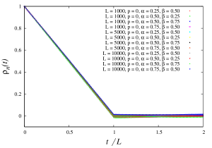
Figure 2: Color online. Finite-size scaling plot of $\rho_{n}(t)$ for $p=0$ parallel-update TASEP in the high-density and low-density phases, for $L=10^{3},5\times 10^{3},10^{4}$ and a variety of $\alpha,\beta$.

Figs. 3 and 4 show finite-size scaling plots of $\rho_{n}(t)$ for $p=0.25,0.5$, assuming the ansatz given by (1) and (25). There is again excellent data collapse, however we note that there is some noticeable curvature near the edge of the support, so that the sharp cusp present in the $p=0$ case becomes smoothed out somewhat for $p>0$. As discussed in section II.2, this does not affect the use of (13) for setting Monte Carlo error bars, but it would be interesting from a theoretical perspective to better understand how this curvature depends on the model parameters $p,\alpha,\beta$ and $L$ (as well as $v_{\max}$; c.f. the discussion in section IV). We remark that many other quantities (including the fundamental diagram) have cusps at $p=0$ which are smoothed out for $p>0$.

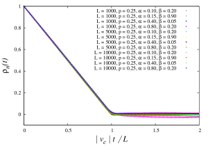
Figure 3: Color online. Finite-size scaling plot of $\rho_{n}(t)$ for $p=0.25$ parallel-update TASEP in the high-density and low-density phases, for $L=10^{3},5\times 10^{3},10^{4}$ and a variety of $\alpha,\beta$. The choices of $\alpha,\beta$ shown correspond to four distinct values of $v_{c}$ providing strong evidence for the conjecture (25).

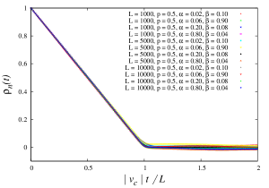
Figure 4: Color online. Finite-size scaling plot of $\rho_{n}(t)$ for $p=0.5$ parallel-update TASEP in the high-density and low-density phases, for $L=10^{3},5\times 10^{3},10^{4}$ and a variety of $\alpha,\beta$. The choices of $\alpha,\beta$ shown correspond to four distinct values of $v_{c}$ providing strong evidence for the conjecture (25).

IV Nagel-Schreckenberg model

An important generalization of the TASEP is the Nagel-Schreckenberg model Nagel and Schreckenberg (1992), in which each particle (vehicle) can move up to $v_{\max}\in\mathbb{N}$ sites per iteration. Although the precise form of the phase diagram depends on $v_{\max}$, the NaSch model exhibits, in general, the same three qualitatively distinct phases as the TASEP Barlovic et al. (2002). We now briefly review the dynamical rules defining the NaSch model. Suppose at time $t\in\mathbb{N}$ a vehicle with speed $v_{t}\in\{0,1,\ldots,v_{\max}\}$ is located on site $x_{t}$, and has headway (number of empty sites to its right) equal to $h_{t}$. Then the maximum speed this vehicle can safely achieve at the next time step is taken to be $v_{\text{safe}}=\min(v_{t}+1,v_{\max},h_{t})$, which allows for unit acceleration provided the speed limit is obeyed and crashes are avoided. Provided $v_{\text{safe}}>0$, a random deceleration is then applied so that with probability $p$ the new speed is $v_{t+1}=v_{\text{safe}}-1$, otherwise $v_{t+1}=v_{\text{safe}}$. Finally, in the bulk of the system, the vehicle hops $v_{t+1}$ sites to its right, so that $x_{t+1}=x_{t}+v_{t+1}$. All vehicles in the bulk of the system are updated in this way in parallel. The bulk dynamics clearly reduces to parallel-update TASEP when $v_{\max}=1$.

It remains to consider the boundary dynamics. We again wish to apply open boundary conditions, however choosing an appropriate implementation of such boundary conditions for the NaSch model is actually surprisingly subtle, and has been an active topic of research over recent years Cheybani et al. (2000a, b); Ding-wei Huang (2001); Barlovic et al. (2002); Jia and Ma (2009); Neumann and Wagner (2009). In particular, it was argued in Barlovic et al. (2002) that in order to observe the maximum-current phase when $v_{\max}>1$ one needs to implement the inflow of vehicles into the system in a rather careful manner.

Since our interest in the present context is confined to the high and low density phases however, we have chosen to implement the boundary conditions in the following simple way. We augment the system, which has sites $1\leq i\leq L$, with two boundary sites; one at $i=0$ and another at $i=L+1$. With probability $\alpha$ a vehicle with speed $v_{\max}$ is inserted on site $0$, and we immediately compute $v_{\text{safe}}$ for this vehicle. If $v_{\text{safe}}>0$ we move the vehicle to site $v_{\text{safe}}$ otherwise we delete it. The output is performed similarly. With probability $1-\beta$ we insert a vehicle on site $L+1$, which then acts as a blockage to vehicles exiting the system. If the rightmost vehicle in the system has $x_{t}\geq L-v_{\max}$ we define its new speed to be $v_{\text{safe}}$ and attempt to move the vehicle to site $x_{t+1}=x_{t}+v_{\text{safe}}$. If $x_{t+1}>L$ the vehicle is removed from the system. When $v_{\max}=1$ the above prescription reduces to the boundary rules for the simple TASEP described in section I.

IV.1 Simulations

We now describe our simulations of the NaSch model as defined above. To our knowledge, no rigorous results are known for $v_{c}$ when $v_{\max}>1$. However, for the deterministic case ($p=0$) we expect that

$$v_{c}=\begin{cases}v_{\max},&\text{low density phase},\\ -1,&\text{high density phase},\\ \end{cases}$$ (26)

for any $v_{\max}$, since in the low-density phase the deterministic movement of vehicles from left to right should control the dynamics, while in the high-density phase we expect that it is the movement of holes (traveling with speed 1) from right to left which is important. More generally, we expect the form (24) to remain valid, but with an unknown function $g$, that will in general depend on $v_{\max}$.

Fig. 5 presents a finite-size scaling plot of $\rho_{n}(t)$ obtained by simulating the NaSch model with $v_{\max}=3$ and $p=0$, with system sizes $L=10^{3}$, $5\times 10^{3}$ and $10^{4}$ and a variety of values of $\alpha,\beta$ corresponding to both the low and high density phases. The data collapse is excellent, providing strong evidence for the ansatz obtained from (1), (3), and (26). As for the case of $p=0$ when $v_{\max}=1$ we note the sharpness of the cusp at $t=L/|v_{c}|$, again suggesting that any corrections to the ansatz (1) are very small.

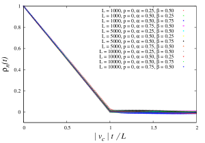
Figure 5: Color online. Finite-size scaling plot of $\rho_{n}(t)$ for $p=0$ NaSch with $v_{\max}=3$ in the high-density and low-density phases, for a variety of choices of $\alpha,\beta$ and $L$. The exact value of $v_{c}$ is unknown in this case but here we chosen $v_{c}$ according to (26).

Each simulation performed consisted of $10^{4}L/|v_{c}|$ iterations (with $v_{c}$ given by (26)), with the first $10^{3}L/|v_{c}|$ time-steps discarded. The above simulations were also performed for $v_{\max}=5$ with identical results.

Finally, we also considered the case of $v_{\max}=3$ with $p=0.25$. For $v_{\max}>1$ and $p>0$ we are not aware of any exact predictions for $v_{c}$, however it seems reasonable to conjecture that $v_{c}$ is independent of $\beta$ ($\alpha$) in the low (high) density phase. We therefore simulated the NaSch model with $v_{\max}=3$, $p=0.25$ and $\alpha=0.25$ at four different values of $\beta>\alpha$, which should then correspond to a single value of $v_{c}$. By considering a single value of $v_{c}$ we can still use a finite-size scaling plot of $\rho_{n}(t)$ to test the conjectures (1) and (3). Fig. 6 provides strong evidence to support their validity at $v_{\max}>1$ and $p>0$. By varying the value of $|v_{c}|$ used to produce the scaling plot of $\rho_{n}(t)$ so that the support edge lay at $|v_{c}|t/L=1$ we obtained $v_{c}\approx 2.65$. We remark that, assuming the validity of (1) and (3), this method can be used as a way to obtain approximate values of $|v_{c}|$ when $v_{\max}>1$ and $p>0$.

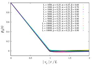
Figure 6: Color online. Finite-size scaling plot of $\rho_{n}(t)$ for $p=0.25$ NaSch with $v_{\max}=3$ in the high-density and low-density phases, for a variety of choices of $\alpha,\beta$ and $L$. The exact value of $v_{c}$ is unknown in this case but here we have set $v_{c}=2.65$.

V Discussion

We have studied the NaSch model in the low and high density phases via Monte Carlo simulation, and found that to a very good approximation the autocorrelation function for the system density behaves as $1-|v_{c}\,t|/L$ with a finite support $[-L/|v_{c}|,L/|v_{c}|]$, where $v_{c}$ is the collective velocity. For the case of $v_{\max}=1$ an exact theoretical result is known for $v_{c}$ for all $p\in[0,1]$. When $v_{\max}>1$ no rigorous results for $v_{c}$ are known, however we conjecture that the when $p=0$ we simply have $v_{c}=v_{\max}$ in the low-density phase and $v_{c}=-1$ in the high-density phase. This result agrees with the exact result in the special case of $v_{\max}=1$ and with numerical simulations for $v_{\max}=3,5$. It seems reasonable to expect that it is valid for all $v_{\max}$ for the deterministic NaSch model.