Perpendicular Ion Heating by Low-Frequency Alfvén-Wave Turbulence in the Solar Wind

Abstract

We consider ion heating by turbulent Alfvén waves (AWs) and kinetic Alfvén waves (KAWs) with wavelengths (measured perpendicular to the magnetic field) that are comparable to the ion gyroradius and frequencies $\omega$ smaller than the ion cyclotron frequency $\Omega$. As in previous studies, we find that when the turbulence amplitude exceeds a certain threshold, an ion’s orbit becomes chaotic. The ion then interacts stochastically with the time-varying electrostatic potential, and the ion’s energy undergoes a random walk. Using phenomenological arguments, we derive an analytic expression for the rates at which different ion species are heated, which we test by simulating test particles interacting with a spectrum of randomly phased AWs and KAWs. We find that the stochastic heating rate depends sensitively on the quantity $\epsilon=\delta v_{\rho}/v_{\perp}$, where $v_{\perp}$ ($v_{\parallel}$) is the component of the ion velocity perpendicular (parallel) to the background magnetic field ${\bf B}_{0}$, and $\delta v_{\rho}$ ($\delta B_{\rho}$) is the rms amplitude of the velocity (magnetic-field) fluctuations at the gyroradius scale. In the case of thermal protons, when $\epsilon\ll\epsilon_{\rm crit}$, where $\epsilon_{\rm crit}$ is a dimensionless constant, a proton’s magnetic moment is nearly conserved and stochastic heating is extremely weak. However, when $\epsilon>\epsilon_{\rm crit}$, the proton heating rate exceeds the cascade power that would be present in strong balanced KAW turbulence with the same value of $\delta v_{\rho}$, and magnetic-moment conservation is violated even when $\omega\ll\Omega$. For the random-phase waves in our test-particle simulations, $\epsilon_{\rm crit}\simeq 0.2$. For protons in low-$\beta$ plasmas, $\epsilon\simeq\beta^{-1/2}\delta B_{\rho}/B_{0}$, and $\epsilon$ can exceed $\epsilon_{\rm crit}$ even when $\delta B_{\rho}/B_{0}\ll\epsilon_{\rm crit}$, where $\beta$ is the ratio of plasma pressure to magnetic pressure. The heating is anisotropic, increasing $v_{\perp}^{2}$ much more than $v_{\parallel}^{2}$ when $\beta\ll 1$. (In contrast, at $\beta\gtrsim 1$ Landau damping and transit-time damping of KAWs lead to strong parallel heating of protons.) At comparable temperatures, alpha particles and minor ions have larger values of $\epsilon$ than protons and are heated more efficiently as a result. We discuss the implications of our results for ion heating in coronal holes and the solar wind.

1. Introduction

Beginning in the 1960s, a number of authors developed steady-state hydrodynamic models of the solar wind, in which the temperature was fixed at the coronal base and the solar wind was heated by thermal conduction (e.g. Parker 1965; Hartle & Sturrock 1968; Durney 1972; Holzer & Leer 1980). For realistic values of the coronal temperature and density, these models were unable to reproduce the large flow velocities of fast-solar-wind streams at 1 AU, suggesting that the fast wind is heated above the coronal base by some additional mechanism. Observational evidence for extended, non-conductive heating has since been provided by measurements from the Ultraviolet Coronagraph Spectrometer (UVCS), which show radially increasing minor-ion temperatures in coronal holes (the open-magnetic-field-line regions from which the fast wind emanates) at heliocentric distances $r$ between $1.5R_{\sun}$ and $3.5R_{\sun}$ (Kohl et al., 1998; Antonucci et al., 2000). Identifying the physical mechanisms responsible for this heating and determining the heating rates of the different particle species are among the major challenges in the study of the solar wind at the present time.

One of the first mechanisms proposed to account for solar-wind heating was turbulence (Coleman, 1968). The importance of turbulent heating is suggested by in situ measurements of ubiquitous, large-amplitude fluctuations in the velocity and magnetic field in the interplanetary medium (Belcher and Davis, 1971; Goldstein et al., 1995; Bruno and Carbone, 2005), as well as the positive correlation between the solar-wind temperature and the amplitude of the fluctuations (Grappin et al., 1990; Vasquez et al., 2007). In addition, the expected rate at which the measured fluctuations dissipate (based on phenomenological turbulence theories) is comparable to the observationally inferred solar-wind heating rate (Smith et al., 2001; Breech et al., 2009; Cranmer et al., 2009). The in situ measurements on which the above studies are based are limited to the locations where spacecraft have flown - that is, to $r\gtrsim 0.3$ AU. However, the velocity and magnetic-field fluctuations are often correlated in the sense of Alfvén waves propagating away from the Sun in the solar-wind frame (Belcher and Davis, 1971; Tu and Marsch, 1995; Bavassano et al., 2000), indicating that these waves originate at or near the Sun, consistent with the idea that turbulent heating remains important as $r$ decreases below $0.3$ AU.

At least two different scenarios for turbulent heating of coronal holes and the solar wind are possible. In the first, magnetic reconnection or some other process launches Alfvén waves into the corona, including waves with $|k_{\parallel}|\gtrsim k_{\perp}$, where $k_{\parallel}$ and $k_{\perp}$ are the components of the wavevector ${\bf k}$ parallel and perpendicular to the local background magnetic field ${\bf B}_{0}$. Given the large Alfvén speed $v_{\rm A}$ in coronal holes ($\gtrsim 10^{3}$ km/s), the frequency $\omega=k_{\parallel}v_{\rm A}$ of such waves exceeds 1 Hz for wavelengths shorter than $\sim 10^{4}$ km. Once such waves enter the corona, nonlinear interactions with coronal density fluctuations [which are inferred from radio observations (Coles and Harmon, 1989)] can convert a significant fraction of the Alfvén wave power into fast magnetosonic waves (Chandran, 2008). The energy in fast magnetosonic waves can then cascade to higher frequencies (Cho and Lazarian, 2002; Svidzinski et al., 2010), generating high-frequency Alfvén waves with $k_{\parallel}>k_{\perp}$ in the process (Chandran, 2005). Although the dissipation of high-frequency fast waves and Alfvén/ion-cyclotron waves could in principle explain the UVCS observations of ion heating (Li and Habbal, 2001; Hollweg and Isenberg, 2002; Markovskii et al., 2010), there is no direct observational evidence that waves with high frequencies and/or $|k_{\parallel}|\gtrsim k_{\perp}$ are present in coronal holes.

An alternative scenario, which we focus on in this paper, involves the launching of much lower-frequency Alfvén waves by convective photospheric motions. An effective $k_{\perp}$ for such waves can be estimated as $2\pi/L_{0}$, where $L_{0}$ is of order the average spacing of either supergranules ($\sim 3\times 10^{4}$ km) or photospheric flux tubes ($\sim 5000$ km). For a wave period $2\pi/(k_{\parallel}v_{\rm A})$ of $10^{3}$ s and an Alfvén speed of $10^{3}$ km/s, the ratio $|k_{\parallel}|/k_{\perp}$ of such waves is $\leq 0.03$. Such highly anisotropic Alfvén waves are inefficient at generating compressive modes (Cho and Lazarian, 2003; Chandran, 2005, 2008). On the other hand, they can interact with oppositely propagating Alfvén waves, causing wave energy to cascade from large scales to small scales, or, equivalently, small $k$ to large $k$, where the fluctuations dissipate, heating the ambient plasma (Iroshnikov, 1963; Kraichnan, 1965). Although the Sun launches only outward-propagating Alfvén waves, the inward-propagating waves required for the Alfvén-wave cascade are generated near the Sun by non-WKB wave reflection arising from the gradient in the Alfvén speed (Heinemann and Olbert, 1980; Velli et al., 1989; Matthaeus et al., 1999; Dmitruk et al., 2002; Cranmer and van Ballegooijen, 2005; Verdini and Velli, 2007; Hollweg and Isenberg, 2007; Verdini et al., 2009a). An important development in the theory of Alfvén-wave turbulence was the discovery that interactions between oppositely propagating Alfvén waves cause wave energy to cascade primarily to larger $k_{\perp}$ and only weakly to larger $|k_{\parallel}|$ (Montgomery and Turner, 1981; Shebalin et al., 1983; Goldreich and Sridhar, 1995). At the dissipation scale, the value of $|k_{\parallel}|/k_{\perp}$ is thus even smaller than at the driving scale $L_{0}$.

This second scenario for solar-wind heating is compelling for a number of reasons. For example, convective photospheric motions inevitably launch low-frequency Alfvén waves into the corona by perturbing the footpoints of open magnetic field lines, and low-frequency Alfvén waves are observed in the corona (Tomczyk et al., 2007) and at $r>0.3$ AU (Belcher and Davis, 1971). In addition, several models have been developed to describe wave reflection and turbulent heating by low-frequency Alfvén waves in the fast solar wind, taking into account the solar-wind velocity, density, and magnetic-field profiles, and incorporating observational constraints on the Alfvén-wave amplitudes; in all of these models, the turbulent heating rate appears to be consistent with the requirements for generating the fast wind (Cranmer and van Ballegooijen, 2005; Cranmer et al., 2007; Chandran and Hollweg, 2009; Verdini et al., 2009b, 2010). We also note that radio observations of density fluctuations provide an upper limit on the heating rate from Alfvén waves in coronal holes, since the Alfvén waves become increasingly compressive with increasing $k$. Although these upper limits rule out fast-wind generation by non-turbulent high-frequency Alfvén/ion-cyclotron waves (unless ${\bf k}$ is nearly parallel to ${\bf B}_{0}$ for all the waves; Hollweg 2000), they are consistent with fast-wind generation by low-frequency (kinetic) Alfvén-wave turbulence with $k_{\perp}\gg k_{\parallel}$ (Harmon and Coles, 2005; Chandran et al., 2009).

Despite these considerations, it is not clear that low-frequency Alfvén-wave turbulence can explain two key observations. First, measurements of the proton and electron temperature profiles in the fast solar wind at $r>0.3$ AU demonstrate that the proton heating rate exceeds the electron heating rate by a modest factor (Cranmer et al., 2009). Similarly, empirically constrained fluid models of coronal holes including thermal conduction suggest that protons receive a substantial fraction ($\sim 0.5$) of the total heating power (Allen et al., 1998). Second, UVCS observations show that minor ions such as ${\rm O}^{+5}$ are heated in such a way that thermal motions perpendicular to ${\bf B}_{0}$ are much more rapid than thermal motions along ${\bf B}_{0}$ (i.e., $T_{\perp}\gg T_{\parallel}$) (Kohl et al., 1998; Antonucci et al., 2000). A similar temperature anisotropy is measured in situ at $r>0.3$ AU for protons in fast-solar-wind streams with $\beta\ll 1$, despite the fact that (double) adiabatic expansion acts to decrease $T_{\perp}/T_{\parallel}$ (Marsch et al., 1982, 2004; Hellinger et al., 2006), where $\beta=8\pi p/B^{2}$ is the ratio of the plasma pressure to the magnetic pressure. Thus, in coronal holes and fast wind with $\beta\ll 1$, ions receive $\gtrsim 1/2$ of the total heating, and ion heating is mostly “perpendicular to the magnetic field.”

Because the rms amplitude of the magnetic-field fluctuation $\delta B$ at the dissipation scale is $\ll B_{0}$, the damping of turbulent fluctuations can be treated, to a first approximation, using the Vlasov-Maxwell theory of linear waves. In this theory, Alfvén waves are virtually undamped when $k_{\perp}\rho_{\rm p}\ll 1$ and $\omega\ll\Omega_{\rm p}$, where $\rho_{\rm p}$ is the rms proton gyroradius and $\Omega_{\rm p}$ is the proton cyclotron frequency. However, as $k_{\perp}\rho_{\rm p}$ increases to values $\gtrsim 1$, the Alfvén waves (AWs) become kinetic Alfvén waves (KAWs), the ions begin to decouple from the electrons, and the waves develop fluctuating electric-field and magnetic-field components parallel to ${\bf B}_{0}$ (Hasegawa and Chen, 1976; Schekochihin et al., 2009). For KAWs with $k_{\parallel}\ll k_{\perp}$ and $\omega\ll\Omega_{\rm p}$, the primary damping mechanisms are Landau damping and/or transit-time damping, which lead to parallel heating of the plasma, not perpendicular heating (Quataert, 1998; Leamon et al., 1999; Cranmer and van Ballegooijen, 2003; Gary and Nishimura, 2004). Moreover, in low-$\beta$ plasmas, the waves damp almost entirely on the electrons, because thermal ions are too slow to satisfy the Landau resonance condition $\omega-k_{\parallel}v_{\parallel}=0$ (Quataert, 1998; Gruzinov, 1998). Thus, if KAWs damp according to linear Vlasov theory, then they are unable to explain the strong perpendicular ion heating that is inferred from observations. This discrepancy casts doubt on the viability of low-frequency AW/KAW turbulence as a mechanism for heating coronal holes and the fast solar wind.

A number of studies have gone beyond linear Vlasov theory to investigate the possibility of perpendicular ion heating by low-frequency AW/KAW turbulence. Johnson and Cheng (2001), Chen et al. (2001), White et al. (2002), and Voitenko and Goossens (2004) investigated the dissipation of mono-chromatic KAWs and AWs with $\omega<\Omega_{\rm p}$, finding that such waves cause perpendicular ion heating if the wave amplitude exceeds a minimum threshold. Dmitruk et al. (2004) and Lehe et al. (2009) simulated test particles propagating in the electric and magnetic fields resulting from direct numerical simulations of magnetohydrodynamic (MHD) turbulence at $0.1\lesssim\beta\lesssim 10$. They both found perpendicular ion heating under some conditions, but Lehe et al. (2009) argued that the perpendicular heating seen in both studies is due to cyclotron resonance and does not apply to the solar wind because it is an artifact of limited numerical resolution. Parashar et al. (2009) found perpendicular ion heating in two-dimensional hybrid simulations of a turbulent plasma, in which ions are treated as particles and electrons are treated as a fluid. In addition, Markovskii and Hollweg (2002) and Markovskii et al. (2006) investigated high-frequency secondary instabilities that are generated by KAWs near the gyroradius scale, and argued that such instabilities may be able to explain the observed perpendicular ion heating.

In this paper, we continue this general line of inquiry and address an important open problem: determining the perpendicular ion heating rate in anisotropic, low-frequency ($\omega<\Omega_{\rm p}$), AW/KAW turbulence as a function of the amplitude of the turbulent fluctuations at the gyroradius scale. In section 2 we develop a phenomenological theory of stochastic ion heating, obtaining an approximate analytic expression for the heating rates of different ion species. We also present simulations of test particles propagating in a spectrum of AWs and KAWs to test our phenomenological theory and to determine the two dimensionless constants that appear in our expression for the heating rate. In section 3 we apply our results to perpendicular ion heating in coronal holes and the fast solar wind.

2. Stochastic Ion Heating by Alfvénic Turbulence at the Gyroradius Scale

We consider ion heating by fluctuations with transverse length scales $\lambda_{\perp}$ (measured perpendicular to ${\bf B}_{0}$) of order the ion gyroradius $\rho=v_{\perp}/\Omega$ (i.e., $k_{\perp}\rho\sim 1$), where $\Omega=qB_{0}/mc$ is the ion cyclotron frequency, and $q$ and $m$ are the ion charge and mass. We assume that $\rho\gtrsim\rho_{\rm p}$, where

$$\rho_{\rm p}=\frac{v_{\perp{\rm p}}}{\Omega_{\rm p}}$$ (1)

is the rms proton gyroradius in the background magnetic field,

$$v_{\perp{\rm p}}=\sqrt{\frac{2k_{\rm B}T_{\rm p}}{m_{\rm p}}}$$ (2)

is the rms perpendicular velocity of protons, $T_{\rm p}$ is the (perpendicular) proton temperature, and $m_{\rm p}$ is the proton mass. If $\rho\gg\rho_{\rm p}$, then the gyro-scale fluctuations are AWs. If $\rho\sim\rho_{\rm p}$, then the gyro-scale fluctuations are KAWs.

We define $\delta v_{\rho}$ and $\delta B_{\rho}$ to be the rms amplitudes of the fluctuating velocity and magnetic-field vectors at $k_{\perp}\rho\sim 1$. Similarly, $\delta E_{\rho}$ and $\delta\Phi_{\rho}$ are the rms amplitudes of the fluctuating electric field and electrostatic potential at $k_{\perp}\rho\sim 1$. We assume that $\delta v_{\rho}$, $\delta B_{\rho}$, $\delta E_{\rho}$, and $\delta\Phi_{\rho}$ are related to one another in the same way that the magnitudes of the fluctuating velocity, magnetic field, electric field, and electrostatic potential are related in a linear (kinetic) Alfvén wave. Thus, since $k_{\perp}\rho_{\rm p}\lesssim 1$,

$$\delta E_{\rho}\simeq\frac{\delta v_{\rho}B_{0}}{c},$$ (3)

$\delta\Phi_{\rho}\sim\rho\delta E_{\rho}$, and

$$q\,\delta\Phi_{\rho}\sim mv_{\perp}\,\delta v_{\rho}.$$ (4)

The fractional change in an ion’s perpendicular kinetic energy $mv_{\perp}^{2}/2$ during a single gyro-period is then given by

$$\frac{2q\,\delta\Phi_{\rho}}{mv_{\perp}^{2}}\sim 2\epsilon,$$ (5)

where

$$\epsilon=\frac{\delta v_{\rho}}{v_{\perp}}.$$ (6)

When $\epsilon\ll 1$, an ion’s kinetic energy is nearly constant during a single gyro-period. If in addition $\delta B_{\rho}\ll B_{0}$, then the ion’s orbit in the plane perpendicular to ${\bf B}_{0}$ closely approximates a closed circle in some suitably chosen reference frame. In this case, the ion possesses an adiabatic invariant of the form $J=\oint pdq$ that is conserved to a high degree of accuracy, where $q$ is the angular coordinate corresponding to the particle’s nearly periodic cyclotron gyration and $p$ is the canonically conjugate momentum (Kruskal, 1962). In the limit of small $\epsilon$, $J$ is approximately equal to the magnetic moment $\mu=mv_{\perp}^{2}/2B$. The near conservation of $J$ implies that perpendicular ion heating is extremely weak. In Appendix A, we present a calculation for electrostatic waves with $k_{\perp}\rho\sim 1$ and $\epsilon\ll 1$ that illustrates how the leading-order terms in the time derivative of $v_{\perp}^{2}$ are unable to cause secular growth in $T_{\perp}$.

On the other hand, as $\epsilon$ increases from 0 to 1, the fractional change in an ion’s perpendicular kinetic energy during a single gyro-period grows to a value of order unity. We treat the spatial variations in the electrostatic potential $\Phi$ at $k_{\perp}\rho\sim 1$ as random or disordered, as is the case in turbulence or a spectrum of many randomly phased waves. Thus, when $\epsilon$ exceeds some threshold (whose value we investigate below), an ion’s orbit in the plane perpendicular to ${\bf B}_{0}$ becomes chaotic. In this case, the ion’s orbit does not satisfy the criteria for the approximate conservation of $J$ (Kruskal, 1962), and perpendicular ion heating becomes possible (Johnson and Cheng, 2001; Chen et al., 2001; White et al., 2002).

To estimate the rate at which ions are heated, we begin by considering the Hamiltonian of a particle of charge $q$ and mass $m$,

$$H=q\Phi+\frac{1}{2m}\left({\bf p}-\frac{q}{c}{\bf A}\right)^{2},$$ (7)

where ${\bf A}$ is the vector potential, and ${\bf p}$ is the canonical momentum. Hamilton’s equations imply that

$$\frac{dH}{dt}=q\frac{\partial\Phi}{\partial t}-\frac{q{\bf v}}{c}\cdot\frac{\partial{\bf A}}{\partial t},$$ (8)

where ${\bf v}=m^{-1}({\bf p}-q{\bf A}/c)$ is the particle’s velocity. The electric field is given by ${\bf E}=-\nabla\Phi-c^{-1}\partial{\bf A}/\partial t$. The second term in equation (8) is $q{\bf v}\cdot{\bf E}_{\rm s}$, where ${\bf E}_{\rm s}=-c^{-1}\partial{\bf A}/\partial t$ is the part of the electric field that has a nonzero curl. In AWs and KAWs with $\omega<\Omega_{\rm p}$ and $k_{\perp}\rho_{\rm p}\lesssim 1$, ${\bf E}_{\rm s}$ is negligible compared to the total electric field in low-$\beta$ plasmas [see equation (46) of Hollweg (1999)], which are our primary focus, and so from here on we neglect the second term in equation (8).

When $\partial\Phi/\partial t>0$, a particle can gain potential energy, kinetic energy, or both. For example, if an ion interacts with an electrostatic wave with wavelength $\gg\rho$ and frequency $\ll\Omega$, then the ion’s guiding center drifts with velocity $c{\bf E}\times{\bf B}_{0}/B_{0}^{2}$. The particle’s kinetic energy undergoes small-amplitude oscillations due to its gyro-motion. However, because its guiding center moves perpendicular to $\nabla\Phi$, there is no significant secular change in its kinetic energy. The ion’s magnetic moment $\mu$ is almost exactly conserved, and the change in its total-energy is almost exactly equal to the change in its potential energy.

On the other hand, if a particle enters a region in which $\partial\Phi/\partial t>0$ and then leaves this region, moving up and down the potential gradient, then it can gain kinetic energy as illustrated in figure 1. The “wire-mesh” surface in the upper panel of this figure represents $\Phi(x_{1},x_{2},t)$ at some initial time, and the lower panel shows $\Phi(x_{1},x_{2},t)$ at a later time. We take the maximum of $\Phi$ to be located at $\sigma=0$, where $\sigma\equiv\sqrt{x_{1}^{2}+x_{2}^{2}}$. We have assumed that $\partial\Phi/\partial t>0$ at $\sigma\lesssim\sigma_{0}$ and $\partial\Phi/\partial t=0$ at $\sigma\gtrsim\sigma_{0}$, where $\sigma_{0}$ is the approximate radius in the $x_{1}-x_{2}$ plane of the “potential-energy hills” that appear in the figure. The thick solid line shows the value of $\Phi$ along the trajectory of a particle moving in a straight line in the $x_{1}-x_{2}$ plane. Because $\partial\Phi/\partial t>0$, the potential-energy hill is shorter when the particle is “climbing up” and higher when the particle is “rolling down.” The particle thus experiences a net gain of kinetic energy from “rolling over the hill.”

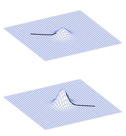
Figure 1.— The potential $\Phi$ in the $x_{1}-x_{2}$ plane at some initial time (upper surface), at a later time (lower surface), and along the trajectory of a particle moving in a straight line in the $x_{1}-x_{2}$ plane (thick solid line). The “potential energy hill” is shorter when the particle rolls to the top, and higher when the particle rolls down, so the particle gains kinetic energy as it rolls over the hill.

We now estimate the rate at which ions are heated by AW or KAW fluctuations with $\lambda_{\perp}\sim\rho$. We note that the condition $\lambda_{\perp}\sim\rho$ is intended to encompass structures with $\lambda_{\perp}=0.5\rho$, which we invoke below when discussing equation (23). However, we ignore fluctuations with $\lambda_{\perp}\gg\rho$ or $\lambda_{\perp}\ll\rho$ throughout this discussion. Although we are interested in stochastic ion orbits, we can still define an effective guiding-center position,

$${\bf R}={\bf r}+\frac{{\bf v}\times{\bf\hat{b}}}{\Omega},$$ (9)

where ${\bf\hat{b}}={\bf B}/B$ and ${\bf r}$ is the ion’s instantaneous position. When $\epsilon\ll 1$, the particle gyrates smoothly about position ${\bf R}$. As $\epsilon$ increases towards 1, the particle’s motion becomes more complicated, but the particle remains within a distance $\sim\rho$ of position ${\bf R}$. Taking the time derivative of equation (9) and using the equation $d{\bf v}/dt=(q/m)({\bf E}+{\bf v}\times{\bf B}/c)$, we obtain the equation

$$\frac{d{\bf R}}{dt}=v_{\parallel}{\bf\hat{b}}+\frac{c{\bf E}\times{\bf B}}{B^{2}}+\dots,$$ (10)

where the ellipsis ($\dots$) represents terms proportional to derivatives of ${\bf B}$, which we ignore in our approximate treatment. During a single cyclotron period, an ion passes through a small number of uncorrelated fluctuations or “structures” of transverse scale $\sim\rho$. Within different structures, the vector $c{\bf E}\times{\bf B}/B^{2}$ has a similar magnitude ($\sim\delta v_{\rho}$) but points in different directions. The time average of $c{\bf E}\times{\bf B}/B^{2}$ over a single cyclotron period is thus somewhat smaller than, but of order, $\delta v_{\rho}$. The time $\Delta t$ required for an ion’s guiding center to move a distance $\rho$ is thus approximately

$$\Delta t\sim\frac{\rho}{\delta v_{\rho}}.$$ (11)

[In writing equation (11), we have assumed that the gyro-scale fluctuations do not oscillate on a time scale $\ll\Delta t$, and we continue to make this assumption in the analysis to follow.] Each time the particle moves a distance $\rho$ perpendicular to ${\bf B}_{0}$, it encounters different and uncorrelated gyro-scale electromagnetic fields. Thus, $d{\bf R}/dt$ decorrelates after a time $\Delta t$, and the particle’s guiding center undergoes a random walk in space with diffusion coefficient $\sim\rho^{2}/\Delta t$.

Similarly, when $\epsilon$ is sufficiently large that the ion’s motion becomes stochastic, the value of $dH/dt$ decorrelates after a time $\Delta t$, and the particle undergoes a random walk in energy. In contrast, as shown in Appendix A, as $\epsilon\rightarrow 0$ the interaction between ions and gyro-scale electrostatic-potential structures is not a Markov process; instead, changes in $H$ are correlated over long times, and to leading order in $\epsilon$ are reversible and bounded. Returning to the stochastic case, we define $\overline{\partial\Phi/\partial t}$ to be the rms value of $\partial\Phi/\partial t$ associated with fluctuations with $\lambda_{\perp}\sim\rho$. The rms change in $H$ during a time $\Delta t$ is then

$$\Delta H\sim q\,\overline{\frac{\partial\Phi}{\partial t}}\,\Delta t.$$ (12)

An ion undergoing stochastic motion can gain kinetic energy in the same way as the particle illustrated in figure 1. If the ion spends a time $\Delta t$ localized within a flux tube of cross-sectional area $\sim\rho^{2}$ and length $\sim|v_{\parallel}|\Delta t$, it exits this flux tube in a random direction. Thus, if $\partial\tilde{\Phi}/\partial t$ is on average positive during this time interval within the flux tube, it does not follow that the ion will move to a region of larger $\tilde{\Phi}$ after a time $\Delta t$, where $\tilde{\Phi}$ is the electrostatic potential associated with fluctuations with $\lambda_{\perp}\sim\rho$. On the contrary, the change in $\tilde{\Phi}$ along the ion’s path is only loosely correlated with the average change in $\tilde{\Phi}$ within the flux tube. As a result, the change in the ion’s kinetic energy during a time $\Delta t$ is of the same order of magnitude as the change in its total energy given in equation (12). Because $\nabla\Phi$ is nearly perpendicular to ${\bf B}$, and because the ion’s guiding center moves perpendicular to ${\bf B}$ by a distance of order $\lambda_{\perp}\sim\rho$ during a time $\Delta t$, the ion’s perpendicular kinetic energy $K_{\perp}=mv_{\perp}^{2}/2$ changes by an amount of order

$$\Delta K_{\perp}\sim\Delta H$$ (13)

during a time $\Delta t$. We discuss the parallel kinetic energy following equation (24) below. We define an effective frequency $\omega_{\rm eff}$ for gyro-scale fluctuations through the equation

$$\overline{\frac{\partial\Phi}{\partial t}}=\omega_{\rm eff}\,\delta\Phi_{\rho}.$$ (14)

For example, if the gyro-scale fluctuations consist of waves with a single frequency $\omega$, then $\omega_{\rm eff}=\omega$. With the use of equations (4) and (11), we can rewrite equation (13) as

$$\Delta K_{\perp}\sim mv_{\perp}\omega_{\rm eff}\rho.$$ (15)

The kinetic-energy diffusion coefficient $D_{K}\sim(\Delta K_{\perp})^{2}/\Delta t$ is then given by

$$D_{K}\sim m^{2}v_{\perp}^{2}\omega_{\rm eff}^{2}\,\delta v_{\rho}\,\rho.$$ (16)

When a single ion undergoes kinetic-energy diffusion, the ion has an equal likelihood of gaining or losing kinetic energy during each “random-walk step” of duration $\Delta t$. On the other hand, if a large population of ions undergoes kinetic-energy diffusion, and if the phase-space density $f$ of ions is a monotonically decreasing function of $K_{\perp}$, then the average value of $K_{\perp}$ increases steadily in time. To distinguish between properties of individual particles and rms quantities within a distribution, we define $v_{\perp{\rm i}}$ to be the rms perpendicular velocity of the ions, which is related to the perpendicular ion temperature $T_{\perp}$ by the equation

$$v_{\perp{\rm i}}=\sqrt{\frac{2k_{\rm B}T_{\perp}}{m}}.$$ (17)

We also define the rms ion gyroradius,

$$\rho_{\rm i}=\frac{v_{\perp{\rm i}}}{\Omega}.$$ (18)

We define $\delta v_{\rm i}$ to be the rms amplitude of the fluctuating fluid velocity at $\lambda_{\perp}\sim\rho_{\rm i}$, and we set

$$\epsilon_{\rm i}=\frac{\delta v_{\rm i}}{v_{\perp{\rm i}}}.$$ (19)

For protons, we define $\delta v_{\rm p}$ ($\delta B_{\rm p}$) to be the fluctuating fluid velocity (magnetic field) at $\lambda_{\perp}\sim\rho_{\rm p}$, and we define

$$\epsilon_{\rm p}=\frac{\delta v_{\rm p}}{v_{\perp{\rm p}}}.$$ (20)

The time scale for the average value of $K_{\perp}$ in a distribution of ions to double is then roughly

$$t_{\rm i}\sim\frac{m^{2}v_{\perp{\rm i}}^{4}}{D_{K{\rm i}}},$$ (21)

where $D_{K{\rm i}}$ is the value of $D_{\rm K}$ for ions with $v_{\perp}=v_{\perp{\rm i}}$ and $\rho=\rho_{\rm i}$. The perpendicular ion heating rate per unit mass is then $Q_{\perp}\sim v_{\perp{\rm i}}^{2}/t_{\rm i}$, or

$$Q_{\perp}\sim\omega_{\rm eff,i}^{2}\,\delta v_{\rm i}\rho_{\rm i},$$ (22)

where $\omega_{\rm eff,i}$ is the value of $\omega_{\rm eff}$ at $\rho=\rho_{\rm i}$.

We now consider what determines the value of $\omega_{\rm eff}$ in anisotropic AW or KAW turbulence. If the turbulence is driven at an “outer scale” $L_{0}$ that is $\gg\rho$, the advection or “sweeping” of structures with $\lambda_{\perp}\sim\rho$ by the outer-scale velocity fluctuations leads to rapid time variations in $\Phi$ at a fixed point in space. On the other hand, these large-scale velocity fluctuations advect both the ions and the small-scale structures in the electric and magnetic fields. Thus, if one considers ions within a flux tube of radius $\sim\rho$ and length $\ll L_{0}$, and if one transforms to a frame of reference moving with the average velocity of that flux tube, then the rapid time variations resulting from large-scale advection disappear. This indicates that large-scale sweeping does not control the rate of ion heating or the value of $\omega_{\rm eff}$ in equation (22). On the other hand, electrostatic-potential structures at scale $\lambda_{\perp}\simeq 0.5\rho$ are advected by velocity fluctuations at the same scale, and there is no frame of reference in which the velocities at $\lambda_{\perp}\simeq 0.5\rho$ vanish at all points along an ion’s gyro-orbit. This advection by velocity fluctuations with $\lambda_{\perp}\simeq 0.5\rho$ causes $\overline{\partial\Phi/\partial t}$ to have a value of $\sim\delta\Phi_{\rm\rho}\delta v_{\rho}/\rho$, which gives

$$\omega_{\rm eff}\sim\frac{\delta v_{\rho}}{\rho},$$ (23)

where we have neglected factors of order unity, such as the ratio between $\delta v_{\rho}$ and the rms amplitude of the velocity fluctuation at $\lambda_{\perp}\simeq 0.5\rho$. Put another way, the advection of electrostatic-potential structures at $\lambda_{\perp}\sim 0.5\rho$, which are rooted in the electron fluid, leads to a partial time derivative of $\Phi$ that ions can feel, and which energizes ions through the process illustrated in figure 1. We note that in “imbalanced” (or cross-helical) AW turbulence, in which the majority of the waves propagate either parallel to ${\bf B}_{0}$ or anti-parallel to ${\bf B}_{0}$, the energy cascade time for the majority waves can greatly exceed $\omega_{\rm eff}^{-1}$, since the majority waves are cascaded by the smaller-amplitude waves propagating in the opposite direction. Nevertheless, even for imbalanced turbulence, the arguments leading to equation (23) continue to hold.

As discussed following equation (6) and in Appendix A, when $\epsilon$ is sufficiently small, the changes in $H$ remain correlated (and largely reversible) over long times, so that the perpendicular heating rate is strongly reduced relative to our estimate in equation (22). To account for this, we introduce a multiplicative suppression factor onto the right-hand side of equation (22) of the form $\exp(-c_{2}/\epsilon_{\rm i})$. We also add an overall coefficient $c_{1}$ to the right-hand side of equation (22) to account for the various approximations we have made. Both $c_{1}$ and $c_{2}$ are dimensionless constants whose values depend upon the nature of the fluctuations (e.g., whether the fluctuations are waves or turbulence, the type of turbulence, etc) and the shape of the ion velocity distribution. Substituting equation (23) into equation (22), we obtain

$$Q_{\perp}=\frac{c_{1}(\delta v_{\rm i})^{3}}{\rho_{\rm i}}\,\exp\left(-\,\frac{c_{2}}{\epsilon_{\rm i}}\right).$$ (24)

We emphasize that for protons in low-$\beta$ plasmas, $\epsilon_{\rm p}\simeq\beta^{-1/2}\delta B_{\rm p}/B_{0}$, and thus $\epsilon_{\rm p}$ can approach unity even if $\delta B_{\rm p}/B_{0}$ remains $\ll 1$.

The change in an ion’s parallel kinetic energy $K_{\parallel}=mv_{\parallel}^{2}/2$ during a time $\Delta t$ due to the parallel electric field $E_{\parallel}$ is $\Delta K_{\parallel}\sim qE_{\parallel}v_{\parallel}\Delta t$. We have restricted our analysis to AWs and KAWs with $\lambda_{\perp}\sim\rho\gtrsim\rho_{\rm p}$ and $\omega^{-1}\gtrsim\Delta t\sim\lambda_{\perp}/\delta v_{\rho}$. This condition on the wave frequency implies that the parallel wavelengths of such fluctuations satisfy the inequality $\lambda_{\parallel}\gtrsim\rho v_{\rm A}/\delta v_{\rho}\gg\lambda_{\perp}$. When $m_{e}/m_{p}<\beta<1$ and $\lambda_{\perp}>\rho_{\rm p}$, $E_{\parallel}/E_{\perp}\sim\rho_{\rm p}^{2}/(\lambda_{\perp}\lambda_{\parallel})$, where $m_{e}$ is the electron mass (Hollweg, 1999) and $E_{\perp}$ is the electric-field component perpendicular to ${\bf B}$. Thus $\Delta K_{\parallel}$ is $\lesssim v_{\parallel}/v_{\rm A}$ times the value of $\Delta K_{\perp}$ in equation (15). For thermal ions in low-$\beta$ plasmas, $v_{\parallel}\ll v_{\rm A}$. Thus, when $\epsilon_{\rm i}$ is sufficiently large that stochastic heating is important, stochastic heating leads primarily to perpendicular ion heating rather than parallel heating. For AWs/KAWs in low-$\beta$ plasmas, the parallel component of the magnetic mirror force is much less than $qE_{\parallel}$ (Hollweg, 1999) and thus does not affect our conclusions regarding anisotropic heating at $\beta\ll 1$.

2.1. Test-Particle Simulations of Proton Heating

To test the above ideas, we have numerically simulated test-particle protons interacting with a spectrum of randomly phased KAWs. The protons’ initial locations are chosen randomly from a uniform distribution within a volume encompassing many wavelengths perpendicular and parallel to ${\bf B}_{0}$. The protons’ initial velocities are drawn randomly from an isotropic Maxwellian distribution of temperature $T_{\rm p}$. For each particle, we solve the equations

$$\frac{d{\bf x}}{dt}={\bf v}$$ (25)

and

$$\frac{d{\bf v}}{dt}=\frac{q}{m}\left({\bf E}+\frac{{\bf v}\times{\bf B}}{c}\right)$$ (26)

using the Bulirsch-Stoer method (Press et al., 1992). We take ${\bf B}=B_{0}{\bf\hat{z}}+{\bf B}_{1}$, where $B_{0}$ is constant. We take ${\bf E}$ and ${\bf B}_{1}$ to be the sum of the electric and magnetic fields from 162 waves with randomly chosen initial phases, with two waves at each of 81 different wave vectors. At each wave vector, there is one wave with $\omega/k_{z}>0$ and a second wave with $\omega/k_{z}<0$. This second wave has the same amplitude as the first, so that there are equal fluxes of waves propagating in the $+z$ and $-z$ directions. The 81 different wave vectors consist of 9 wave vectors at each of nine different values of $k_{\perp}$, denoted $k_{\perp j}$. The $k_{\perp j}$ can be expressed in terms $\rho_{\rm p}$. In particular, the values $\psi_{j}=\ln(k_{\perp j}\rho_{\rm p})$ are uniformly spaced between $-4/3$ and $4/3$; i.e., $\psi_{j}=-4/3+j/3$, with $j=0,1,\dots,8$. We regard the values $\psi_{j}$ as corresponding to cell centers in a uniform grid in $\psi=\ln(k_{\perp}\rho_{\rm p})$, with grid spacing $\Delta\psi=1/3$. The middle three grid cells, with $j=\mbox{3, 4, and 5}$, thus correspond to an interval of width unity in $\ln(k_{\perp})$ space centered on $k_{\perp}\rho_{\rm p}=1$. We define the rms amplitudes of the gyro-scale velocity and magnetic-field fluctuations $\delta v_{\rm p}$ and $\delta B_{\rm p}$ in our simulations by taking the rms values of the ${\bf E}\times{\bf B}$ velocity and magnetic-field fluctuation resulting from the KAWs in these middle three grid cells. At each $k_{\perp j}$ we include 9 different values of the azimuthal angle $\phi$ in $k$ space, $\phi_{l}=2\pi l/9$, where $l=0,1,\dots,8$. At each $k_{\perp j}$ there is only a single value of $k_{\parallel}$, which we denote $k_{\parallel j}$. We choose $k_{\parallel 4}$ so that the frequency at $k_{\perp}=k_{\perp 4}$ and $k_{\parallel}=k_{\parallel 4}$ equals $k_{\perp 4}\delta v_{\rho}$. The linear frequency of our gyro-scale KAWs is thus comparable to the value of $\omega_{\rm eff}$ given in equation (23) for KAW turbulence at $k_{\perp}\rho_{\rm p}\sim 1$. We then set

$$\frac{k_{\parallel j}}{k_{\parallel 4}}=\left\{\begin{array}[]{ll}(k_{\perp j}/k_{\perp 4})^{2/3}&\mbox{ if $0\leq j<4$}\\ (k_{\perp j}/k_{\perp 4})^{1/3}&\mbox{ if $4<j\leq 8$}\end{array}\;.\right.$$ (27)

Our formula for $k_{\parallel j}$ at $j<4$ is chosen so that the wave periods are comparable to the energy cascade time scales in the critical-balance theory of Goldreich and Sridhar (1995), while the formula for $j>4$ is chosen so that the wave periods match the nonlinear time scales in the critical-balance theory of Cho and Lazarian (2004). All waves at the same $k_{\perp}$ have the same amplitude, and (since there are the same number of waves at each $k_{\perp j}$) we take the amplitude of the magnetic-field fluctuation in each wave to be $\propto k_{\perp}^{-1/3}$ for $k_{\perp}\rho_{\rm p}<1$ and $\propto k_{\perp}^{-2/3}$ for $k_{\perp}\rho_{\rm p}>1$, again motivated by the theories of Goldreich and Sridhar (1995) and Cho and Lazarian (2004).

The relative amplitudes of the different components of ${\bf E}$ and ${\bf B}_{1}$ for each wave are taken from the two-fluid theory of Hollweg (1999). To apply this theory, we choose plasma parameters that are characteristic of coronal holes. In particular, we set $\beta_{e}=8\pi nk_{\rm B}T_{\rm e}/B_{0}^{2}=0.003$, $v_{\rm A}=0.003c$, and $T_{\rm e}=0.5T_{\rm p}$, where $n$ is the electron number density (equal to the proton number density), and $T_{\rm e}$ is the electron temperature.

Using the above procedures, we have carried out seven simulations with different values for the overall normalization of the wave amplitudes, with $\delta B_{\rm p}/B_{0}$ ranging from $4.8\times 10^{-3}$ to $1.9\times 10^{-2}$. Given the polarization properties of KAWs and our method for constructing the wave spectra, the value of $\delta v_{\rm p}/v_{\rm A}$ is $1.19$ times the value of $\delta B_{\rm p}/B_{0}$ in each simulation. The wave frequencies reach their maximum values in the largest-$\delta B_{\rm p}/B_{0}$ simulation. In this simulation, $\omega=0.29\Omega_{\rm p}$ at $k_{\perp}\rho_{\rm p}=1$, and $\omega=0.82\Omega_{\rm p}$ at the maximum value of $k_{\perp}\rho_{\rm p}$, which is $3.79$. Although this maximum frequency is close to $\Omega_{\rm p}$, the cyclotron resonance condition $\omega-k_{\parallel}v_{\parallel}=l\Omega_{\rm p}$ (where $l$ is any integer) is not satisfied, because the parallel thermal speed of the protons is only $0.055v_{\rm A}$ and $k_{\parallel}\ll k_{\perp}$. For most of the waves in these simulations, $\omega\ll\Omega_{\rm p}$.

We determine the perpendicular proton heating rate per unit mass $Q_{\perp{\rm p}}$ in the simulations by plotting $\langle v_{\perp}^{2}\rangle$ versus time, fitting this plot to a straight line to determine $(d/dt)\langle v_{\perp}^{2}\rangle$, and then setting $Q_{\perp{\rm p}}=0.5(d/dt)\langle v_{\perp}^{2}\rangle$, where $\langle\dots\rangle$ indicates an average over the $10^{3}$ particles in each simulation. When fitting the plot of $\langle v_{\perp}^{2}\rangle$ versus time, we ignore the first $10$ cyclotron periods, because during the first couple gyro-periods the particles undergo a modest apparent heating as they “pick up” some portion of the ${\bf E}\times{\bf B}$ velocity of the waves. We find that after $\langle v_{\perp}^{2}\rangle$ increases by between 20% and 40%, the heating rate starts to decrease for two reasons. First, the small-$v_{\perp}$ part of the velocity distribution flattens, after which this part of the distribution is no longer heated as effectively. Second, as $\langle v_{\perp}^{2}\rangle$ increases, $\epsilon_{\rm p}$ decreases. We neglect this later stage of weaker heating when constructing our fits to the $\langle v_{\perp}^{2}(t)\rangle$ plots, so that the measured heating rates correspond to Maxwellian distributions. (For the smallest values of $\delta v_{\rm p}$, we do not observe a second stage of weaker heating, because the test-particle velocity distributions do not change very much during the simulations, which last $10^{4}\Omega_{\rm p}^{-1}$.) We illustrate this procedure in figure 2 for a run with $\delta v_{\rm p}/v_{\perp{\rm p}}=0.15$. In this case, we determine $Q_{\perp{\rm p}}$ from the slope of the long-dashed line, which is our fit to the $\langle v_{\perp}^{2}\rangle$ data over the interval $10<\Omega_{\rm p}t<10^{3}$.

Figure 2.— $v_{\perp}^{2}$ and $v_{\parallel}^{2}$ averaged over the $10^{3}$ particles in a simulation with $\delta v_{\rm p}/v_{\perp{\rm p}}=0.15$, $\beta_{e}=0.003$, $v_{\rm A}=0.003c$, and $T_{\rm e}=0.5T_{\rm p}$. The two solid-line curves correspond to our basic numerical method. We determine $Q_{\perp{\rm p}}$ in this simulation from the slope of the long-dashed line. The short-dashed line shows $\langle v_{\parallel}^{2}\rangle$ in a modified simulation with the same parameters in which ${\bf E}$ is replaced by ${\bf E}^{\prime}={\bf E}+{\bf\hat{b}}(E_{z}-{\bf\hat{b}}\cdot{\bf E})$.

In figure 3 we plot the values of $Q_{\perp{\rm p}}$ for several different values of $\epsilon_{\rm p}$. Each $\times$ in this figure corresponds to a separate simulation with a different value of $\delta v_{\rm p}$ but the same initial proton temperature. The solid line is the proton heating rate from equation (24) with $c_{1}=0.75$ and $c_{2}=0.34$; that is,

$$Q_{\perp{\rm p}}=\frac{0.75(\delta v_{\rm p})^{3}}{\rho_{\rm p}}\,\exp\left(-\,\frac{0.34}{\epsilon_{\rm p}}\right).$$ (28)

We expect the constants $c_{1}$ and $c_{2}$ to be fairly insensitive to variations in $\beta_{\rm e}$, $T_{\rm p}/T_{\rm e}$, and $v_{\rm A}/c$ (at least within the range of solar-wind-relevant parameters), in which case $Q_{\perp{\rm p}}$ depends on the plasma parameters primarily through the explicit $\rho_{\rm p}$ and $\epsilon_{\rm p}$ terms in equation (28). The values of $c_{1}$ and $c_{2}$ in equation (28) presuppose the presence of a broad spectrum of AWs and KAWs bracketing the perpendicular wavenumber $k_{\perp}=(\rho_{\rm p})^{-1}$, encompassing at a minimum the range $0.3\lesssim k_{\perp}\rho_{\rm p}\lesssim 3$. A spectrum of at least this width is probably present in the solar wind, the only uncertainty being the value of the dissipation wavenumber beyond which the wave power spectrum decreases exponentially with increasing $k_{\perp}$. If the simulations described in this section are repeated without the smallest three values of $k_{\perp}$ and without the largest three values of $k_{\perp}$ (keeping the wave amplitudes fixed at the middle three values of $k_{\perp}$), then the proton orbits become less stochastic, and $Q_{\perp{\rm p}}$ decreases significantly. (The exact amount by which $Q_{\perp{\rm p}}$ decreases depends upon the value of $\epsilon_{\rm p}$.) We have omitted waves at $k_{\perp}\rho_{\rm p}<0.26$ and $k_{\perp}\rho_{\rm p}>3.8$, but we expect that waves at such scales do not have a strong effect on perpendicular ion heating, provided $\omega$ is sufficiently small that the cyclotron resonance condition can not be satisfied. It is possible that in some cases strongly turbulent fluctuations with $k_{\perp}\rho_{\rm p}\gg 1$ and nonlinear time scales $\sim\Omega_{\rm p}^{-1}$ could heat ions through a broadened cyclotron resonance, but a detailed investigation of this process is beyond the scope of this study.

We reiterate that the values of $c_{1}$ and $c_{2}$ in equation (28) are not universal, but instead depend on the type of fluctuations that are present. In true turbulence (as opposed to random-phased waves), the value of $c_{2}$ may be smaller than in our simulations (indicating stronger heating), because a significant fraction of the cascade power may be dissipated in coherent structures in which the fluctuating fields are larger than their rms values (Dmitruk et al., 2004).

Figure 3.— Numerical results (plotted with $\times$s) for the perpendicular heating rate $Q_{\perp{\rm p}}$ for test-particle protons interacting with a spectrum of randomly phased KAWs. The solid line is equation (28), and the dashed line is equation (28) with the “$\mu$ conservation” factor $\exp(-0.34/\epsilon_{\rm p})$ replaced with unity.

The lower solid-line curve in figure 2 plots $\langle v_{\parallel}^{2}\rangle$ versus time in the simulation with $\epsilon_{\rm p}=0.15$, $\beta_{e}=0.003$, $v_{\rm A}=0.003c$, and $T_{\rm e}=0.5T_{\rm p}$. During the interval $10<\Omega_{\rm p}t<2200$, the increase in $\langle v_{\parallel}^{2}\rangle$ is about one-fourth the increase in $\langle v_{\perp}^{2}\rangle$. However, most of the increase in $\langle v_{\parallel}^{2}\rangle$ is an artifact of our numerical method, which equates the parallel electric fields of the waves with the $z$ component of the electric field in the simulation, and the perpendicular electric field of the waves with the $x$ and $y$ components of the electric field in the simulation. The local magnetic field in our simulations, however, is not parallel to the $z$ axis, but instead has nonzero $x$ and $y$ components resulting from the magnetic-field fluctuations. As a result, part of the perpendicular wave electric field is converted into a parallel electric field in the simulation, artificially enhancing the parallel electric field seen by the particles. To eliminate this effect, we have repeated this simulation replacing the local electric field ${\bf E}$ seen by each particle with the adjusted electric field ${\bf E}^{\prime}={\bf E}+{\bf\hat{b}}(E_{z}-{\bf\hat{b}}\cdot{\bf E})$, where ${\bf\hat{b}}={\bf B}/B$ and ${\bf B}$ is the local value of the magnetic field. In this new simulation, the parallel electric field ${\bf\hat{b}}\cdot{\bf E}^{\prime}$ is the sum of the parallel electric fields of the individual waves in the simulation and does not include any contribution from the perpendicular electric fields of the individual waves. The value of $\langle v_{\parallel}^{2}\rangle$ in this modified simulation, shown as a dashed line in figure 2, does not increase significantly during the course of the simulation (in fact it decreases slightly), consistent with our argument above that parallel heating is weak when $\beta\ll 1$.

2.2. Proton Heating at $k_{\perp}\rho_{\rm p}\sim 1$ as a Fraction of the Turbulent Cascade Power

The cascade power per unit mass at $k_{\perp}\rho_{\rm p}\sim 1$, which we denote $\Gamma$, depends upon whether the turbulence is “balanced” or “imbalanced,” where balanced (imbalanced) turbulence involves equal (unequal) fluxes of waves propagating parallel to ${\bf B}_{0}$ and anti-parallel to ${\bf B}_{0}$. In balanced KAW turbulence,

$$\Gamma=C_{\rm K}^{-3/2}\left(\frac{\delta v_{\rm p}}{\rho_{\rm p}}\right)\left(\frac{\delta B_{\rm p}}{B_{0}}\right)^{2}v_{\rm A}^{2},$$ (29)

where $C_{\rm K}$ is a dimensionless constant (Howes et al. 2008a). It can be inferred from the numerical simulations of Howes et al. (2008b) that $C_{\rm K}=2.0$ (G. Howes, private communication). In the simulations of section 2.1, $\delta B_{\rm p}/B_{0}=0.84\delta v_{\rm p}/v_{\rm A}$, and we make the approximation that this same ratio is characteristic of KAW turbulence in general. Combining equations (28) and (29), we obtain

$$\frac{Q_{\perp{\rm p}}}{\Gamma}=3.0\,\exp\left(-\,\frac{0.34}{\epsilon_{\rm p}}\right).$$ (30)

We expect that $C_{K}$, like the constants $c_{1}$ and $c_{2}$, depends only weakly on $\beta$, $T_{\rm p}/T_{\rm e}$, and $v_{\rm A}/c$ (at least for solar-wind-relevant parameters), so that the numerical constants 3.0 and 3.4 in equation (30) are relatively insensitive to the plasma parameters. Equation (30) implies that perpendicular proton heating by KAWs with $k_{\perp}\rho_{\rm p}\sim 1$ absorbs $\geq 1/2$ of the cascade power at $k_{\perp}\rho_{\rm p}\sim 1$ when $\epsilon_{\rm p}$ exceeds

$$\epsilon_{\rm crit}=0.19\;.$$ (31)

The cascade power in imbalanced AW turbulence is smaller than in balanced AW turbulence with the same total fluctuation energy, because the AW energy cascade requires interactions between oppositely propagating waves (Iroshnikov, 1963; Kraichnan, 1965). At $k_{\perp}\rho_{\rm p}\sim 1$, KAWs propagating in the same direction can interact nonlinearly with one another, but the importance of such interactions relative to interactions between oppositely propagating waves is not well known. Despite this uncertainty, we expect that if AW/KAW turbulence is imbalanced at $k_{\perp}\rho_{\rm p}\sim 1$, then the cascade power at $k_{\perp}\rho_{\rm p}\sim 1$ is less than in equation (29). On the other hand, it is unlikely that imbalance strongly affects $Q_{\perp{\rm p}}$ if $\delta v_{\rm p}$ is held fixed (except for particles with $v_{\parallel}\sim\pm v_{\rm A}$, as discussed in section 2.4). We thus expect perpendicular proton heating to absorb at least 50% of the cascade power at $k_{\perp}\rho_{\rm p}\sim 1$ in imbalanced turbulence even when $\epsilon_{\rm p}$ is somewhat smaller than $0.19$.

2.3. Proton Heating versus Electron Heating by KAWs with $k_{\perp}\rho_{\rm p}\sim 1$

Stochastic proton heating removes energy from KAW fluctuations with $k_{\perp}\rho_{\rm p}\sim 1$, resulting in an effective damping rate for these fluctuations, which we denote $\gamma_{\rm p}$. The value of $\gamma_{\rm p}$ is given by the relation

$$2\gamma_{\rm p}{\cal E}_{\rm w}=Q_{\perp{\rm p}},$$ (32)

where ${\cal E}_{\rm w}$ is the energy per unit mass of the KAW fluctuations at $k_{\perp}\rho_{\rm p}\sim 1$. The factor of 2 in equation (32) is included to make $\gamma_{\rm p}$ analogous to a linear wave damping rate, in the sense that the rate at which linear waves lose energy is twice the product of the damping rate and the wave energy. To estimate the value of $\gamma_{\rm p}$ in AW/KAW turbulence, we use the test-particle calculations in section 2.1 for a spectrum of randomly phased KAWs. We take ${\cal E}_{\rm w}$ to be the energy per unit mass of the full spectrum of waves in these simulations. (This choice leads to a conservative estimate of $\gamma_{\rm p}$, since the damping is likely concentrated in the subset of the waves with $k_{\perp}\rho_{\rm p}\gtrsim 1$.) On the other hand, we continue to define $(\delta v_{\rm p})^{2}$ as the mean-square ${\bf E}\times{\bf B}$ velocity associated with KAWs with values of $k_{\perp}$ lying within a logarithmic interval of width unity centered on $k_{\perp}\rho_{\rm p}=1$. With these definitions, ${\cal E}_{\rm w}=2.1(\delta v_{\rm p})^{2}$ in all of the simulations in section 2.1. Combining equations (28) and (32), we obtain

$$\gamma_{\rm p}=0.18\epsilon_{\rm p}\Omega_{\rm p}\,\exp\left(-\,\frac{0.34}{\epsilon_{\rm p}}\right).$$ (33)

In low-$\beta$ plasmas, small-amplitude KAWs with $k_{\perp}\rho_{\rm p}=1$ and $\omega\ll\Omega_{\rm p}$ undergo electron Landau damping but negligible linear proton damping (Quataert, 1998; Gruzinov, 1998; Gary and Nishimura, 2004). Using the numerical method described by Quataert (1998) and Howes et al. (2008a), we numerically solve the full hot-plasma dispersion relation to find the electron damping rate $\gamma_{\rm e}$ of KAWs with $k_{\perp}\rho_{\rm p}=1$ and $\omega\ll\Omega_{\rm p}$ for a range of values of $k_{\parallel}$, $T_{\rm p}/T_{\rm e}$, $\beta_{\rm p}$, and $v_{\rm A}/c$, where $\beta_{\rm p}=8\pi nk_{\rm B}T_{\rm p}/B_{0}^{2}$. We find that if $m_{\rm e}/m_{\rm p}\ll\beta_{\rm e}\ll 1$, $v_{\rm A}\ll c$, and $0.1\lesssim T_{\rm p}/T_{\rm e}\lesssim 10$, then the damping rate at $k_{\perp}\rho_{\rm p}=1$ is well fit by the formula $\gamma_{\rm e}=9.5\times 10^{-3}(T_{\rm e}/T_{\rm p})^{1/2}\beta_{\rm p}^{-1/2}|k_{\parallel}v_{\rm A}|$, or equivalently

$$\gamma_{\rm e}=9.5\times 10^{-3}\epsilon_{\rm p}\chi^{-1}\left(\frac{T_{\rm e}}{\beta_{\rm p}T_{\rm p}}\right)^{1/2}\Omega_{\rm p},$$ (34)

where $\chi\equiv k_{\perp}\delta v_{\rm p}/|k_{\parallel}v_{\rm A}|$. In some theories of strong MHD turbulence $\chi\sim 1$ (Goldreich and Sridhar, 1995; Boldyrev, 2006). This condition, some times referred to as critical balance, may characterize AW/KAW fluctuations in coronal holes and the solar wind at $k_{\perp}\rho_{\rm p}\sim 1$. On the other hand, if the frequencies of the waves launched by photospheric motions are sufficiently small, then AW/KAW turbulence at a heliocentric distance of a few solar radii may be more “two-dimensional” than in critical-balance models, with smaller values of $k_{\parallel}$ and a larger value of $\chi$.

Combining equations (33) and (34), we obtain

$$\frac{\gamma_{\rm p}}{\gamma_{\rm e}}=19\,\chi\,\left(\frac{\beta_{\rm p}T_{\rm p}}{T_{\rm e}}\right)^{1/2}\exp\left(-\,\frac{0.34}{\epsilon_{\rm p}}\right).$$ (35)

The ratio $\gamma_{\rm p}/\gamma_{\rm e}$ approximates the ratio of the proton heating rate to the electron heating rate resulting from KAW fluctuations at $k_{\perp}\rho_{\rm p}\sim 1$ in the low-$\beta$ conditions present in coronal holes and the near-Sun solar wind. (At $\beta\gtrsim 1$, linear KAW damping on the protons becomes important, increasing the proton heating rate.) We note that if the damping time scales $\gamma_{\rm p}^{-1}$ and $\gamma_{\rm e}^{-1}$ are both much longer than the energy cascade time at $k_{\perp}\rho_{\rm p}\sim 1$, then most of the fluctuation energy will cascade past the proton-gyroradius scale to smaller scales. In that case, the division of the turbulent heating between protons and electrons will depend primarily upon how fluctuations dissipate at $k_{\perp}\rho_{\rm p}\gg 1$.

2.4. How the Heating Rate Depends on $q$, $m$, $\beta$, and $v_{\parallel}/v_{\rm A}$

If we re-run our simulations, keeping only waves with $\omega/k_{z}>0$, and consider a thermal distribution of test-particle protons with a nonzero average velocity equal to $v_{\rm A}\hat{z}$, then the perpendicular heating rate is strongly reduced. This is because the electric field of an Alfvén wave (or KAW with $\lambda_{\perp}\sim\rho_{p}$) vanishes (or is strongly reduced) in a reference frame moving at speed $v_{\rm A}$ in the same direction as the wave along the background magnetic field. This effect may explain the observation that the perpendicular heating of $\alpha$ particles in the solar wind is reduced when the differential flow velocity of $\alpha$ particles relative to protons (in the anti-Sunward direction) approaches $v_{\rm A}$ (Kasper et al., 2008), at least in regions where anti-Sunward propagating KAWs dominate over Sunward-propagating KAWs.

If we hold $\delta B_{\rm p}/B_{0}$ fixed but increase $\beta_{\rm p}$ to 1, then the perpendicular proton heating rate is dramatically reduced, because $\epsilon_{\rm p}=\delta v_{\rm p}/v_{\perp}\sim\beta^{-1/2}\delta B_{\rm p}/B_{0}$ decreases by a large factor. On the other hand, the protons in these $\beta_{\rm p}\sim 1$ simulations undergo significant parallel heating, consistent with results from linear theory (Quataert, 1998) and recent test-particle simulations of ions propagating in numerically simulated MHD turbulence (Lehe et al., 2009).

If we re-run our simulations but use ${\rm O}^{+5}$ ions instead of protons (but with the same temperature as the protons), then the perpendicular heating rate is much larger. This is in large part because $\epsilon$ is larger for ${\rm O}^{+5}$ (and other heavy ions) than for protons at the same temperature, a point to which we return in section 3. Another reason for enhanced heavy-ion heating can be seen from equation (21). We rewrite this equation with the aid of equation (23), increasing $t_{\rm i}$ by $\exp(c_{2}/\epsilon_{\rm i})$ for the same reasons that we reduced $Q_{\perp}$ by this same factor in equation (24), to obtain

$$t_{\rm i}\sim\frac{v_{\perp{\rm i}}^{2}\rho_{\rm i}}{(\delta v_{\rm i})^{3}}\,\exp\left(\frac{c_{2}}{\epsilon_{\rm i}}\right).$$ (36)

In a number of theories of MHD turbulence, the ratio $(\delta v_{\rho{\rm i}})^{3}/\rho_{\rm i}$ is relatively (or completely) insensitive to the value of $\rho_{\rm i}$, provided $\rho_{\rm i}$ is in the inertial range of the turbulence. On the other hand, for ion species at equal temperatures, $v_{\perp{\rm i}}^{2}$ is inversely proportional to the ion mass. Thus, even aside from the exponential factor in equation (36), the heating time scale is shorter for heavier ions than for lighter ions at the same temperature.

Finally, if we repeat the simulations of section 2.1 for test-particle ions with $\rho_{\rm i}\gg\rho_{\rm p}$, and with values of $k_{\perp}\rho_{\rm i}$ centered on 1 so that the gyro-scale fluctuations are now AWs, we recover similar values for the perpendicular heating rate per unit mass. Stochastic perpendicular ion heating thus does not require the particular polarization properties of KAWs, but operates for both KAWs and AWs, as we have argued in our heuristic derivation of equation (24).

2.5. Lack of Perpendicular Heating by AWs with $k_{\perp}\rho_{\rm i}\ll 1$

In turbulent flows, the rms variation in the velocity across a perpendicular scale $\lambda_{\perp}$, denoted $\delta v_{\lambda_{\perp}}$, typically increases as some positive power of $\lambda_{\perp}$ when $\lambda_{\perp}$ is in the inertial range. As a result, the variation in the electrostatic potential across an ion’s gyro-orbit is dominated by the fluctuations at the large-scale end of the inertial range, suggesting that these large-scale fluctuations might make an important contribution to the perpendicular heating rate. This suggestion, however, is incorrect, because AWs with $k_{\perp}\rho\ll 1$ cause an ion’s guiding center to drift smoothly at velocity $c{\bf E}\times{\bf B}/B^{2}$, but do not cause an ion’s motion to become chaotic. If one transforms to a reference frame that moves at the velocity $c{\bf E}\times{\bf B}/B^{2}$ evaluated at the ion’s guiding-center position, then the variation in $q\Phi$ across the ion’s gyroradius is a small fraction of $mv_{\perp}^{2}/2$. The ion’s trajectory in the plane perpendicular to ${\bf B}_{0}$ in this frame is approximately a closed circle, and the ion’s magnetic moment $\mu$ is then nearly conserved (Kruskal, 1962).

3. Perpendicular Ion Heating in Coronal Holes and the Fast Solar Wind

As shown in the previous section, the stochastic ion heating rate is a strongly increasing function of $\epsilon_{\rm i}=\delta v_{\rm i}/v_{\perp\rm i}$. For fixed turbulence properties, the value of $\epsilon_{\rm i}$ depends upon the ion charge $q=Ze$, the ion mass $m=Am_{\rm p}$, and the perpendicular ion temperature $T_{\perp}$. For example, if we take the rms amplitude of the turbulent velocity fluctuation at transverse scale $\lambda_{\perp}$ to be given by

$$\delta v_{\lambda_{\perp}}=\alpha v_{\rm A}\left(\frac{\lambda_{\perp}}{L_{0}}\right)^{a}$$ (37)

for $\rho_{\rm p}<\lambda_{\perp}<L_{0}$, where $\alpha$ and $a$ are dimensionless constants and $L_{0}$ is the outer scale or driving scale of the turbulence, then

$$\epsilon_{\rm i}=\alpha\left(\frac{T_{\rm p}}{T_{\perp}\mu_{\rm p}\beta_{\rm p}}\right)^{(1-a)/2}\frac{A^{(1+a)/2}}{Z^{a}}\left(\frac{d_{\rm p}}{L_{0}}\right)^{a},$$ (38)

where $d_{\rm p}=v_{\rm A}/\Omega_{\rm p}$ is the proton inertial length, $\beta_{\rm p}=8\pi n_{\rm p}k_{\rm B}T_{\rm p}/B^{2}$, $n_{\rm p}$ is the proton density, $T_{\rm p}$ is the proton temperature, and $\mu_{\rm p}$ is the mean molecular weight per proton; that is, the mass density is $\mu_{\rm p}n_{\rm p}m_{\rm p}$, and the Alfvén speed is $B/\sqrt{4\pi\mu_{\rm p}n_{\rm p}m_{\rm p}}$. If the velocity power spectrum $P_{k}^{(v)}$ is $\propto k_{\perp}^{-c_{3}}$ for $L_{0}^{-1}<k_{\perp}<\rho_{\rm i}^{-1}$, then

$$a=\frac{c_{3}-1}{2}.$$ (39)

To investigate the possible role of stochastic ion heating in coronal holes and the fast solar wind, we evaluate equation (38) as a function of heliocentric distance $r$ using observationally constrained profiles for the density, temperature, and field strength. We take $n_{\rm p}$ to be given by equation (4) of Feldman et al. (1997), which describes coronal holes out to several solar radii, plus an additional component proportional to $r^{-2}$:

$$n_{\rm p}(r)=\left(\frac{3.23\times 10^{8}}{d^{15.6}}+\frac{2.51\times 10^{6}}{d^{3.76}}+\frac{1.85\times 10^{5}}{d^{2}}\right)\mbox{ cm}^{-3},$$ (40)

where $d=r/R_{\sun}$. Equation (40) gives $n_{\rm p}=4\mbox{ cm}^{-3}$ at 1 AU. We set

$$T_{\rm p}=3\times 10^{6}\mbox{ K}\cdot\left[\frac{1-(2/3)\exp(-d/1.5)}{(1+0.1d)^{0.8}}\right],$$ (41)

which leads to a proton temperature that is $10^{6}$ K at the coronal base, between $2\times 10^{6}$ K and $3\times 10^{6}$ K in coronal holes, and $\sim 2.5\times 10^{5}$ K at 1 AU. We take the magnetic field strength to be (Hollweg and Isenberg, 2002)

$$B_{0}=\left[\frac{1.5(f_{\rm max}-1)}{d^{6}}+\frac{1.5}{d^{2}}\right]\mbox{ Gauss},$$ (42)

with $f_{\rm max}$ (the super-radial expansion factor) equal to 5. We determine the rms amplitude of the fluctuating wave velocity at the outer scale, $\delta v_{L_{0}}=\alpha v_{\rm A}$, using the analytical model of Chandran and Hollweg (2009), which describes the propagation of low-frequency Alfvén waves launched outward from the Sun, taking into account non-WKB wave reflections arising from Alfvén-speed gradients as well as the cascade and dissipation of wave energy arising from nonlinear wave-wave interactions. In particular, we set $\delta v_{L_{0}}$ equal to the value of $\delta v_{\rm rms}$ plotted with a solid line in figure 6 of Chandran and Hollweg (2009) (the curve corresponding to their “extended model”). We take $L_{0}$ to be $10^{4}$ km at the coronal base [the limit $d\rightarrow 1$ in equation (42)], and to be proportional to $B^{-1/2}$.

We consider three different values for the spectral index $c_{3}$: 5/3, 3/2, and 6/5. The value $c_{3}=5/3$ is suggested by in situ measurements of magnetic-field fluctuations in the solar wind (Matthaeus and Goldstein, 1982; Bruno and Carbone, 2005), as well as some theoretical and numerical studies of MHD turbulence (Goldreich and Sridhar, 1995; Cho and Vishniac, 2000). The value $c_{3}=3/2$ is motivated by a different set of theoretical and numerical studies (Boldyrev, 2006; Mason et al., 2006; Perez and Boldyrev, 2009), as well as recent in situ observations of the velocity power spectrum in the solar wind (Podesta et al., 2007; Podesta and Bhattacharjee, 2009). The third value, $c_{3}=1.2$, follows from recent numerical simulations of reflection-driven Alfvén-wave turbulence in coronal holes and the fast solar wind (Verdini et al., 2009b). In these simulations, $c_{3}=1.2$ at $r<1.2R_{\sun}$, and $c_{3}$ gradually increases towards $5/3$ with increasing $r$.

Figure 4.— The values of $\epsilon_{\rm i}=\delta v_{\rm i}/v_{\perp{\rm i}}$ from equation (38) as a function of heliocentric distance for ${\rm H}^{+}$, ${\rm He}^{++}$, and ${\rm O}^{+5}$. For this figure, we assume that $T_{\perp}=T_{\rm p}$ for ${\rm He}^{++}$ and ${\rm O}^{+5}$ and that the one-dimensional velocity power spectrum $P_{k}^{(v)}$ is $\propto k_{\perp}^{-c_{3}}$. From bottom to top, the three curves in each plot correspond to $c_{3}=5/3$, $c_{3}=3/2$, and $c_{3}=1.2$.

In figure 4, we plot $\epsilon_{\rm i}$ for ${\rm H}^{+}$, ${\rm He}^{++}$, and ${\rm O}^{+5}$ assuming $\mu_{\rm p}=1.2$. Although alpha particles and minor ions are observed to be hotter than protons in the fast solar wind, we have set all the ion temperatures equal to $T_{\rm p}$ to investigate the relative heating rates of different ion species that start out at the same temperature. Figure 4 illustrates the general point that $\epsilon_{\rm i}$ depends strongly on the spectral index $c_{3}$. In particular, decreasing $c_{3}$ by 28% from 5/3 to 1.2 increases $\epsilon_{\rm i}$ by a factor of $>10$ at all radii shown for all three ion species. Because $Q_{\perp}$ depends strongly on $\epsilon_{\rm i}$, $Q_{\perp}$ is extremely sensitive to the value of $c_{3}$. For example, for protons, if $c_{3}=1.2$, then $\epsilon_{\rm p}\simeq 0.2$ except at $r<1.5R_{\sun}$. The approximations leading to equation (30) imply that $Q_{\perp{\rm p}}/\Gamma=0.55$ when $\epsilon_{\rm p}=0.2$ (where $\Gamma$ is the cascade power at $k_{\perp}\rho_{\rm p}\sim 1$), indicating that perpendicular proton heating absorbs a substantial fraction of the turbulent heating power when $c_{3}\lesssim 1.2$. On the other hand, if $c_{3}=5/3$, then $\epsilon_{\rm p}<0.02$ and $Q_{\perp{\rm p}}/\Gamma$ in equation (30) is $<1.2\times 10^{-7}$.

A second general point illustrated by figure 4 is that when $c_{3}$ is fixed, $\epsilon_{\rm i}$ depends only weakly on $r$ for $2R_{\sun}<r<1\mbox{ AU}$. As a result, given our assumptions, a large radial variation in $\epsilon$ within this range of $r$ requires a radial variation in the spectral index $c_{3}$. As mentioned above, the numerical simulations of Verdini et al. (2009b) found $c_{3}\simeq 1.2$ at $r<1.2R_{\sun}$, with $c_{3}$ increasing towards 5/3 with increasing $r$. In addition, radio observations show that the density-fluctuation power spectrum is significantly flatter at $r=5R_{\sun}$ than at $r>10R_{\sun}$ (Markovskii and Hollweg, 2002; Harmon and Coles, 2005). These observations and numerical simulations raise the possibility that $c_{3}$ is significantly smaller (and that $Q_{\perp{\rm p}}/\Gamma$ is much larger) close to the Sun than at $\sim 1\mbox{ AU}$. However, the inertial range of reflection-driven AW turbulence in coronal holes is still not well understood. Likewise, the relation between the density power spectrum and the velocity power spectrum in the imbalanced AW turbulence found in coronal holes is not clear. The $r$-dependence of $c_{3}$ thus remains uncertain.

A third point illustrated by figure 4 is that $\epsilon_{\rm i}$ is significantly larger for ${\rm He}^{++}$ and ${\rm O}^{+5}$ than for protons at the same temperature. For example, at equal temperatures, protons and alpha particles have the same gyroradius, and $\epsilon_{\alpha}=2\epsilon_{\rm p}$, where $\epsilon_{\alpha}$ is the value of $\epsilon_{\rm i}$ for alpha particles. Because of the strong dependence of $Q_{\perp}$ on $\epsilon_{\rm i}$, it is possible that the perpendicular heating rate per unit volume from stochastic heating by gyro-scale fluctuations is larger for alpha particles than for protons, even though Helium comprises only $\sim 20\%$ of the mass in the solar wind. Depending on the values of $c_{2}$ and $c_{3}$, it is also possible that Helium absorbs a significant fraction of the turbulent cascade power in the solar wind. In addition, the comparatively large value of $\epsilon_{\rm i}$ for ${\rm O}^{+5}$ may explain why ${\rm O}^{+5}$ ions are observed to be so much hotter than protons in the solar corona (Kohl et al., 1998; Antonucci et al., 2000), and likewise for other minor ions.

4. Conclusion

When an ion interacts with turbulent AWs and/or KAWs, and when the amplitudes of the fluctuating electromagnetic fields at $\lambda_{\perp}\sim\rho$ are sufficiently large, the ion’s orbit becomes chaotic, and the ion undergoes stochastic perpendicular heating. The parameter that has the largest effect on the heating rate is $\epsilon=\delta v_{\rho}/v_{\perp}$, where $\delta v_{\rho}$ is the rms amplitude of the velocity fluctuation at $\lambda_{\perp}\sim\rho$. In the limit $\epsilon\rightarrow 0$, the ion’s magnetic moment is nearly conserved, and perpendicular ion heating is extremely weak. On the other hand, as $\epsilon$ increases towards unity, magnetic moment conservation is violated, and stochastic perpendicular heating becomes increasingly strong.

Using phenomenological arguments, we have derived an analytic formula for the perpendicular heating rate $Q_{\perp}$ for different ion species. This formula (equation (24)) contains two dimensionless constants, $c_{1}$ and $c_{2}$, whose values depend on the nature of the fluctuations (e.g., waves versus turbulence, the slope of the power spectrum) and the shape of the ion velocity distribution. Using test-particle simulations, we numerically evaluate these constants for the case in which a Maxwellian distribution of protons interacts with a spectrum of random-phase AWs and KAWs at perpendicular wavenumbers in the range $0.264<k_{\perp}\rho_{\rm p}<3.79$, where $\rho_{\rm p}$ is the rms proton gyroradius in the background magnetic field ${\bf B}_{0}$. The particular form of the wave power spectrum that we choose for these simulations is motivated by the “critical balance” theories of Goldreich and Sridhar (1995) and Cho and Lazarian (2004). For this case, $c_{1}=0.75$ and $c_{2}=0.34$. The proton heating rate $Q_{\perp{\rm p}}$ can be compared to the cascade power $\Gamma$ that would be present at $k_{\perp}\rho_{\rm p}\sim 1$ in “balanced” (see section 2.2) AW/KAW turbulence with the same value of $\delta v_{\rm p}$. When $c_{1}=0.75$ and $c_{2}=0.34$, the ratio $Q_{\perp{\rm p}}/\Gamma$ exceeds $1/2$ when $\epsilon_{\rm p}>\epsilon_{\rm crit}=0.19$, where $\epsilon_{\rm p}$ is the value of $\epsilon$ for thermal protons.

Our expression for $Q_{\perp{\rm p}}/\Gamma$ (equation (30)) may differ from the value of $Q_{\perp{\rm p}}/\Gamma$ in the solar wind for two main reasons. First, our formula for $\Gamma$ does not take into account “imbalance” (see section 2.2), which affects the relation between $\Gamma$ and $\delta v_{\rm p}$ in a way that is not yet understood. Second, in true turbulence (as opposed to randomly phased waves), a significant fraction of the cascade power may be dissipated in coherent structures in which the fluctuating fields are larger than their rms values (Dmitruk et al., 2004). Proton orbits in the vicinity of such structures are more stochastic than in average regions, and thus $c_{2}$ may be smaller in AW/KAW turbulence than in our test-particle simulations, indicating stronger heating. The perpendicular heating rate is very sensitive to the value of $c_{2}/\epsilon_{\rm p}$; our test-particle simulations are consistent with $Q_{\perp{\rm p}}/\Gamma$ being $\propto\exp(-c_{2}/\epsilon_{\rm p})$. Thus, decreasing $c_{2}$ leads to a large increase in $Q_{\perp{\rm p}}/\Gamma$ when $\epsilon_{\rm p}<c_{2}$. Decreasing $c_{2}$ also decreases $\epsilon_{\rm crit}$, the value of $\epsilon_{\rm p}$ at which $Q_{\perp{\rm p}}/\Gamma=1/2$; it follows from equations (24) and (29) that if $C_{K}\simeq 2$, $\delta B_{\rm p}/B_{0}\simeq 0.84\delta v_{\rm p}/v_{\rm A}$, and $c_{1}\simeq 1$, then $\epsilon_{\rm crit}\simeq c_{2}/2$.

When $\beta\ll 1$, stochastic proton heating by AW/KAW turbulence at $k_{\perp}\rho_{\rm p}\sim 1$ increases $T_{\perp}$ much more than $T_{\parallel}$. In contrast, linear proton damping of KAWs with $\omega\ll\Omega_{\rm p}$ and $k_{\perp}\rho_{\rm p}\sim 1$ leads almost entirely to parallel heating, and is only significant when the proton thermal speed is $\gtrsim v_{\rm A}$; i.e., when $\beta_{\rm p}\gtrsim 1$ (Quataert, 1998). If we assume that (nonlinear) stochastic heating and linear wave damping are the only dissipation mechanisms for low-frequency AW/KAW turbulence, then we arrive at the following conclusions about how the cascade power in AW/KAW turbulence is partitioned between parallel and perpendicular heating, and between protons and electrons:

1. If $\beta_{\rm p}\ll 1$ and $\epsilon_{\rm p}\ll\epsilon_{\rm crit}$, then proton heating is negligible and electrons absorb most of the cascade power.

2. If $\beta_{\rm p}\ll 1$ and $\epsilon_{\rm p}\gtrsim\epsilon_{\rm crit}$, then parallel proton heating is negligible, and AW/KAW turbulence leads to a combination of electron heating and perpendicular proton heating.

3. If $\beta_{\rm p}\gtrsim 1$ and $\epsilon_{\rm p}\ll\epsilon_{\rm crit}$, then perpendicular proton heating is negligible, and AW/KAW turbulence results in a combination of electron heating and parallel proton heating.

4. If $\beta_{\rm p}\gtrsim 1$ and $\epsilon_{\rm p}\gtrsim\epsilon_{\rm crit}$, then perpendicular proton heating, parallel proton heating, and electron heating each receives an appreciable fraction of the cascade power.

KAW turbulence at $k_{\perp}\rho_{\rm p}\sim 1$ fluctuates over length (time) scales much greater than $\rho_{\rm e}$ ($\Omega_{\rm e}^{-1}$), where $\rho_{\rm e}$ ($\Omega_{\rm e}$) is the thermal-electron gyroradius (cyclotron frequency). Because of this, an electron’s magnetic moment is nearly conserved when it interacts with KAW turbulence at $k_{\perp}\rho_{\rm p}\sim 1$. Electron heating by KAW turbulence at $k_{\perp}\rho_{\rm p}\sim 1$ is thus primarily parallel heating. On the other hand, some of the fluctuation energy may cascade to scales $\ll\rho_{\rm p}$. The way that turbulence is dissipated at such scales is not yet well understood.

To determine the dependence of $\epsilon_{\rm i}$ (the value of $\epsilon$ for thermal ions) on heliocentric distance $r$ for different ion species in the fast solar wind, we adopt a simple analytic model for the radial profiles of the solar-wind proton density, proton temperature, and magnetic field strength. We then apply the analytical model of Chandran and Hollweg (2009), which describes the radial dependence of the rms amplitudes of Alfvén waves at the outer scale $L_{0}$ of the turbulence, and assume that the velocity power spectrum $P_{k}^{(v)}$ is $\propto k_{\perp}^{-c_{3}}$ for $L_{0}^{-1}<k_{\perp}<\rho_{\rm p}^{-1}$. We find that the value of $\epsilon_{\rm i}$ for protons, Helium, and minor ions depends strongly on $c_{3}$. However, for a fixed value of $c_{3}$, $\epsilon_{\rm i}$ is relatively insensitive to $r$ for $2R_{\sun}<r<\mbox{ 1 AU}$.

We are not yet able to determine with precision the perpendicular heating rates of different ion species as a function of $r$ because of the uncertainties in the values of $c_{2}$ and $c_{3}$ in the solar wind, and because of the large sensitivity of the heating rates to these quantities. However, if we assume that the value of $c_{2}$ for protons in the solar wind is close to the value of 0.34 in our test-particle simulations, then we arrive at the following two conclusions. First, perpendicular proton heating is a negligible fraction of the turbulent cascade power in the bulk of the explored solar wind, in which $c_{3}$ is measured to be in the range of 1.5 - 1.7. Second, if stochastic proton heating is important close to the Sun, then $c_{3}$ must be significantly smaller close to the Sun than at 1 AU. (For example, if $c_{3}=1.2$, then $Q_{\perp{\rm p}}/\Gamma\gtrsim 0.5$ for $2R_{\sun}\lesssim r<100R_{\sun}$.)

We find that alpha particles and minor ions undergo much stronger stochastic heating than protons, in large part part because the value of $\epsilon_{\rm i}$ is larger for these ions than for protons at equal temperatures. Depending on the values of $c_{2}$ and $c_{3}$, the stochastic heating rate per unit volume in the solar wind may be larger for Helium than for protons, even though Helium comprises only $\sim 20\%$ of the solar-wind mass. Figure 4 suggests that stochastic heating is important for alpha particles and minor ions even if $c_{3}$ is as large as 3/2, since $\epsilon_{\rm i}$ is then $\gtrsim 0.1$ over a wide range of $r$. However, further investigations into the value of $c_{3}$ close to the Sun and the value of $c_{2}$ for (non-random-phase) AW/KAW turbulence are needed in order to develop a more complete and accurate picture of stochastic ion heating in the solar wind.

Appendix A Leading-Order Conservation of the First Adiabatic Invariant When $k_{\perp}\rho\sim 1$ and $\epsilon\ll 1$

In this appendix, we consider the interaction between ions and low-frequency, 2D ($k_{\parallel}=0$), electrostatic fluctuations with $k_{\perp}\rho\sim 1$. We assume that $\epsilon\ll 1$, neglect magnetic-field fluctuations, and show that the leading-order non-vanishing terms in $dH/dt$ are unable to cause secular perpendicular ion heating. We set ${\bf B}=B_{0}{\bf\hat{z}}$, where $B_{0}$ is a constant. The time derivative of the ion’s guiding-center position, defined in equation (9), is then given by

$$\frac{d{\bf R}}{dt}=v_{z}{\bf\hat{z}}+\frac{c{\bf E}\times\hat{z}}{B_{0}}.$$ (A1)

Since $\epsilon\ll 1$, the particle’s orbit in the $xy$-plane during a single gyroperiod is approximately a circle of radius $\rho=v_{\perp}/\Omega$. We assume that $\Phi$ varies slowly in time, on a time scale of $\sim\epsilon^{-1}\Omega^{-1}$, with $\partial\Phi/\partial z=0$. We introduce two related forms of “gyro-averages.” First, if $h$ is some physical property of a particle, such as its energy or guiding-center velocity, then we define the gyro-average of $h$ to be

$$\langle h(t)\rangle=\frac{\Omega}{2\pi}\int_{t-\pi/\Omega}^{t+\pi/\Omega}h(t_{1})\,dt_{1}.$$ (A2)

Second, for a general function of position and time $g({\bf r},t)$ satisfying $\partial g/\partial z=0$, we define the gyro-average of $g({\bf r},t)$ for particles with perpendicular velocity $v_{\perp}$ and guiding center ${\bf R}$ to be given by

$$\langle g({\bf r},t)\rangle_{{\bf R},v_{\perp}}\equiv\frac{1}{2\pi}\int_{0}^{2\pi}g\mbox{\large\bf(}{\bf R}+{\bf s}(\theta),t\mbox{\large\bf)}\,d\theta,$$ (A3)

where ${\bf s}={\bf\hat{x}}\rho\cos(\theta)+{\bf\hat{y}}\rho\sin(\theta)$ is the vector illustrated in figure 5.

Figure 5.— In the small-$\epsilon$ limit, an ion’s trajectory in the $xy$ plane is approximately a circle centered on its guiding-center position ${\bf R}$.

To simplify the notation, we define

$$\overline{g}({\bf R},t)\equiv\langle g({\bf r},t)\rangle_{{\bf R},v_{\perp}},$$ (A4)

where the functional dependence of $\overline{g}$ on $v_{\perp}$ is not explicitly written. If $g$ varies slowly in time at a fixed point in space (e.g., on the time scale $\epsilon^{-1}\Omega^{-1}$), then $\overline{g}({\bf R},t)$ is (to leading order in $\epsilon$) equivalent to a time average over one cyclotron period of $g({\bf r},t)$ evaluated at the position ${\bf r}(t)$ of a particle with guiding center ${\bf R}$:

$$\overline{g}({\bf R},t)=\frac{\Omega}{2\pi}\int_{t-\pi/\Omega}^{t+\pi/\Omega}g\mbox{\large\bf(}{\bf r}(t_{1}),t_{1}\mbox{\large\bf)}\,dt_{1}.$$ (A5)

Thus, if we take the gyro-average of the “particle property” $d{\bf R}/dt$ in equation (A1) using equation (A2), we find that

$$\left\langle\frac{d{\bf R}}{dt}\right\rangle=v_{\rm z}{\bf\hat{z}}+\frac{c}{B_{0}}\langle{\bf E}({\bf r},t)\rangle_{{\bf R},v_{\perp}}\times{\bf\hat{z}}.$$ (A6)

We consider electrostatic fluctuations with $\partial{\bf A}/\partial t=0$, and thus, ${\bf E}=-\nabla\Phi$. Omitting the explicit time dependence of $\Phi$ and $\overline{\Phi}$ to simplify the notation, we can write the gyro-average of $\partial\Phi/\partial x$ as

$$\left\langle\frac{\partial\Phi}{\partial x}\right\rangle_{{\bf R},v_{\perp}}=\lim_{\delta\rightarrow 0}\left\langle\frac{\Phi({\bf r}+{\bf\hat{x}}\delta)-\Phi({\bf r})}{\delta}\right\rangle_{{\bf R},v_{\perp}}=\lim_{\delta\rightarrow 0}\frac{\overline{\Phi}({\bf R}+{\bf\hat{x}}\delta)-\overline{\Phi}({\bf R})}{\delta}=\frac{\partial\overline{\Phi}}{\partial x^{\prime}}$$ (A7)

where ${\bf\hat{x}}$ is a unit vector in the $x$ direction, and $\partial/\partial x^{\prime}$ denotes a partial derivative with respect to the x-component of the guiding-center position ${\bf R}$. Equation (A6) can thus be re-written as

$$\left\langle\frac{d{\bf R}}{dt}\right\rangle=v_{\rm z}{\bf\hat{z}}-\frac{c}{B_{0}}\nabla^{\prime}\overline{\Phi}\times{\bf\hat{z}},$$ (A8)

where $\nabla^{\prime}$ indicates a gradient with respect to the coordinates of the guiding-center position ${\bf R}$. Since we have assumed $\partial/\partial z=0$, equation (A8) implies that $\langle d{\bf R}/dt\rangle\cdot\nabla^{\prime}\overline{\Phi}=0$.

We now integrate equation (8) for an integral number of cyclotron periods, from $t_{\rm a}$ to $t_{\rm b}=t_{\rm a}+N\delta t$, where $\delta t=2\pi/\Omega$ and $N\geq\epsilon^{-1}$. We define $t_{0}=t_{\rm a}+\delta t/2$ and $t_{j}=t_{j-1}+\delta t$ for any integer $j$. Since we have assumed that $\partial{\bf A}/\partial t=0$, the integral of equation (8) can be written

$$H(t_{\rm b})-H(t_{\rm a})=q\sum_{j=0}^{N-1}\int_{t_{j}-\delta t/2}^{t_{j}+\delta t/2}\frac{\partial\Phi}{\partial t}\,dt.$$ (A9)

In analogy to equation (A7), it is straightforward to show that $\overline{\partial\Phi/\partial t}=(\partial/\partial t)\overline{\Phi}$. We can thus re-write equation (A9) as

$$H(t_{\rm b})-H(t_{\rm a})=q\sum_{j=0}^{N-1}\,\frac{\partial\overline{\Phi}}{\partial t}\mbox{\large\bf(}{\bf R}(t_{j}),t_{j}\mbox{\large\bf)}\,\delta t.$$ (A10)

The time scale on which $\overline{\Phi}\mbox{\large\bf(}{\bf R}(t),t\mbox{\large\bf)}$ changes by a factor of order unity is $\epsilon^{-1}\delta t$. This is because $\Phi$ changes slowly in time at a fixed point in space, $k_{\perp}\rho\sim 1$, and $d{\bf R}/dt\sim\epsilon v_{\perp}$. As a result $\partial\overline{\Phi}/\partial t$ is approximately constant within each time interval of duration $\delta t$. The right-hand side of equation (A10) is therefore a discrete approximation of the integral of $q\partial\overline{\Phi}/\partial t$ from $t_{\rm a}$ to $t_{\rm b}$, with a fractional error of order $\epsilon$, so that

$$H(t_{\rm b})-H(t_{\rm a})=q\int_{t_{\rm a}}^{t_{\rm b}}\frac{\partial}{\partial t}\,\overline{\Phi}\mbox{\large\bf(}{\bf R}(t),t\mbox{\large\bf)}\,dt+\dots,$$ (A11)

where the ellipsis ($\dots$) represents corrections that are higher order in $\epsilon$. The right-hand side of equation (A11) can be re-written in terms of the total time derivative of $\Phi$, yielding

$$H(t_{\rm b})-H(t_{\rm a})=q\int_{t_{\rm a}}^{t_{\rm b}}\frac{d}{dt}\,\overline{\Phi}\mbox{\large\bf(}{\bf R}(t),t\mbox{\large\bf)}\,dt\>-\>q\int_{t_{\rm a}}^{t_{\rm b}}\frac{d{\bf R}}{dt}\cdot\nabla^{\prime}\overline{\Phi}\mbox{\large\bf(}{\bf R}(t),t\mbox{\large\bf)}\,dt+\dots$$ (A12)

Since $\nabla^{\prime}\overline{\Phi}$ is nearly constant during a single time interval of duration $\delta t$, the second integral on the right-hand side of equation (A12) satisfies the relation

$$\int_{t_{\rm a}}^{t_{\rm b}}\frac{d{\bf R}}{dt}\cdot\nabla^{\prime}\overline{\Phi}\mbox{\large\bf(}{\bf R}(t),t\mbox{\large\bf)}\,dt=\sum_{j=0}^{N-1}\left(\int_{t_{j}-\delta t/2}^{t_{j}+\delta t/2}\frac{d{\bf R}}{dt}\,dt\right)\cdot\nabla^{\prime}\overline{\Phi}\mbox{\large\bf(}{\bf R}(t_{j}),t_{j}\mbox{\large\bf)}+\dots$$ (A13)

The integral within parentheses on the right-hand side of equation (A13) is equivalent to $\langle d{\bf R}/dt\rangle\,\delta t$ evaluated at $t=t_{j}$. From equation (A8), $\langle d{\bf R}/dt\rangle\cdot\nabla^{\prime}\overline{\Phi}=0$. Thus, the right-hand side of equation (A13) and the second integral on the right-hand side of equation (A12) vanish to leading order in $\epsilon$. Equation (A12) thus becomes

$$H(t_{\rm b})-H(t_{\rm a})=q\overline{\Phi}\mbox{\large\bf(}{\bf R}(t_{\rm b}),t_{\rm b}\mbox{\large\bf)}-q\overline{\Phi}\mbox{\large\bf(}{\bf R}(t_{\rm a}),t_{\rm a}\mbox{\large\bf)}+\dots$$ (A14)

The right-hand side of equation (A14) remains $\lesssim q\delta\Phi_{\rho}$, regardless of how large the interval $(t_{\rm b}-t_{\rm a})$ becomes. Thus, to leading order in $\epsilon$, there is no secular change in the particle energy $H$, consistent with the near-conservation of the first adiabatic invariant in the small-$\epsilon$, small-$\omega/\Omega$ limits.

References

- (1)
- Allen et al. (1998) Allen L A, Habbal S R and Hu Y Q 1998 J. Geophys. Res. 103, 6551–+.
- Antonucci et al. (2000) Antonucci E, Dodero M A and Giordano S 2000 Sol. Phys. 197, 115–134.
- Barnes (1966) Barnes A 1966 Physics of Fluids 9, 1483–1495.
- Bavassano et al. (2000) Bavassano B, Pietropaolo E and Bruno R 2000 J. Geophys. Res. 105, 15959–15964.
- Belcher and Davis (1971) Belcher J W and Davis, Jr. L 1971 J. Geophys. Res. 76, 3534–3563.
- Boldyrev (2006) Boldyrev S 2006 Physical Review Letters 96(11), 115002–+.
- Breech et al. (2009) Breech B, Matthaeus W H, Cranmer S R, Kasper J C and Oughton S 2009 Journal of Geophysical Research (Space Physics) 114, 9103–+.
- Bruno and Carbone (2005) Bruno R and Carbone V 2005 Living Reviews in Solar Physics 2, 4–+.
- Chandran (2005) Chandran B D G 2005 Physical Review Letters 95(26), 265004–+.
- Chandran (2008) Chandran B D G 2008 Physical Review Letters 101(23), 235004–+.
- Chandran and Hollweg (2009) Chandran B D G and Hollweg J V 2009 ApJ 707, 1659–1667.
- Chandran et al. (2009) Chandran B D G, Quataert E, Howes G G, Xia Q and Pongkitiwanichakul P 2009 ApJ 707, 1668–1675.
- Chen et al. (2001) Chen L, Lin Z and White R 2001 Physics of Plasmas 8, 4713–4716.
- Cho and Lazarian (2002) Cho J and Lazarian A 2002 Physical Review Letters 88, 245001.
- Cho and Lazarian (2003) Cho J and Lazarian A 2003 MNRAS 345, 325–339.
- Cho and Lazarian (2004) Cho J and Lazarian A 2004 ApJ 615, L41–L44.
- Cho and Vishniac (2000) Cho J and Vishniac E T 2000 ApJ 539, 273–282.
- Coleman (1968) Coleman P J 1968 ApJ 153, 371.
- Coles and Harmon (1989) Coles W A and Harmon J K 1989 ApJ 337, 1023–1034.
- Cranmer et al. (2009) Cranmer S R, Matthaeus W H, Breech B A and Kasper J C 2009 ApJ 702, 1604–1614.
- Cranmer and van Ballegooijen (2003) Cranmer S R and van Ballegooijen A A 2003 ApJ 594, 573–591.
- Cranmer and van Ballegooijen (2005) Cranmer S R and van Ballegooijen A A 2005 Astrophysical Journal Supplement 156, 265–293.
- Cranmer et al. (2007) Cranmer S R, van Ballegooijen A A and Edgar R J 2007 ApJS 171, 520–551.
- Dmitruk et al. (2002) Dmitruk P, Matthaeus W H, Milano L J, Oughton S, Zank G P and Mullan D J 2002 ApJ 575, 571–577.
- Dmitruk et al. (2004) Dmitruk P, Matthaeus W H and Seenu N 2004 ApJ 617, 667–679.
- Durney (1972) Durney B R 1972 J. Geophys. Res. 77, 4042–4051.
- Feldman et al. (1997) Feldman W C, Habbal S R, Hoogeveen G and Wang Y 1997 J. Geophys. Res. 102, 26905–26918.
- Gary and Nishimura (2004) Gary S P and Nishimura K 2004 Journal of Geophysical Research 109, 2109.
- Goldreich and Sridhar (1995) Goldreich P and Sridhar S 1995 Astrophysical Journal 438, 763–775.
- Goldstein et al. (1995) Goldstein M L, Roberts D A and Matthaeus W H 1995 ARA&A 33, 283–326.
- Grappin et al. (1990) Grappin R, Mangeney A and Marsch E 1990 J. Geophys. Res. 95, 8197–8209.
- Gruzinov (1998) Gruzinov A V 1998 ApJ 501, 787–+.
- Harmon and Coles (2005) Harmon J K and Coles W A 2005 Journal of Geophysical Research (Space Physics) 110, 3101–+.
- Hartle and Sturrock (1968) Hartle R E and Sturrock P A 1968 ApJ 151, 1155.
- Hasegawa and Chen (1976) Hasegawa A and Chen L 1976 Physics of Fluids 19, 1924–1934.
- Heinemann and Olbert (1980) Heinemann M and Olbert S 1980 J. Geophys. Res. 85, 1311–1327.
- Hellinger et al. (2006) Hellinger P, Trávníček P, Kasper J C and Lazarus A J 2006 Geophys. Res. Lett. 33, 9101–+.
- Hollweg (1978) Hollweg J V 1978 Geophys. Res. Lett. 5, 731–734.
- Hollweg (1999) Hollweg J V 1999 J. Geophys. Res. 104, 14811–14820.
- Hollweg (2000) Hollweg J V 2000 J. Geophys. Res. 105, 7573–7582.
- Hollweg and Isenberg (2002) Hollweg J V and Isenberg P A 2002 Journal of Geophysical Research (Space Physics) 107, 1147–+.
- Hollweg and Isenberg (2007) Hollweg J V and Isenberg P A 2007 Journal of Geophysical Research (Space Physics) 112, 8102–+.
- Holzer and Leer (1980) Holzer T E and Leer E 1980 J. Geophys. Res. 85, 4665–4679.
- Howes, Cowley, Dorland, Hammett, Quataert and Schekochihin (2008) Howes G G, Cowley S C, Dorland W, Hammett G W, Quataert E and Schekochihin A A 2008 Journal of Geophysical Research (Space Physics) 113, 5103–+.
- Howes, Dorland, Cowley, Hammett, Quataert, Schekochihin and Tatsuno (2008) Howes G G, Dorland W, Cowley S C, Hammett G W, Quataert E, Schekochihin A A and Tatsuno T 2008 Physical Review Letters 100(6), 065004–+.
- Iroshnikov (1963) Iroshnikov P S 1963 AZh 40, 742–+.
- Johnson and Cheng (2001) Johnson J R and Cheng C Z 2001 Geophys. Res. Lett. 28, 4421–4424.
- Kasper et al. (2008) Kasper J C, Lazarus A J and Gary S P 2008 Physical Review Letters 101(26), 261103–+.
- Kohl et al. (1998) Kohl J L, Noci G, Antonucci E, Tondello G, Huber M C E, Cranmer S R, Strachan L, Panasyuk A V, Gardner L D, Romoli M, Fineschi S, Dobrzycka D, Raymond J C, Nicolosi P, Siegmund O H W, Spadaro D, Benna C, Ciaravella A, Giordano S, Habbal S R, Karovska M, Li X, Martin R, Michels J G, Modigliani A, Naletto G, O’Neal R H, Pernechele C, Poletto G, Smith P L and Suleiman R M 1998 Astrophysical Journal Letters 501, L127.
- Kraichnan (1965) Kraichnan R H 1965 Physics of Fluids 8, 1385.
- Kruskal (1962) Kruskal M 1962 Journal of Mathematical Physics 3, 806–828.
- Leamon et al. (1999) Leamon R J, Smith C W, Ness N F and Wong H K 1999 J. Geophys. Res. 104, 22331–22344.
- Lehe et al. (2009) Lehe R, Parrish I J and Quataert E 2009 ArXiv e-prints .
- Li and Habbal (2001) Li X and Habbal S R 2001 J. Geophys. Res. 106, 10669–10680.
- Markovskii and Hollweg (2002) Markovskii S A and Hollweg J V 2002 Journal of Geophysical Research 107, 21.
- Markovskii et al. (2006) Markovskii S A, Vasquez B J, Smith C W and Hollweg J V 2006 ApJ 639, 1177–1185.
- Markovskii et al. (2010) Markovskii S, Vasquez B and Chandran B 2010 Perpendicular proton heating due to energy cascade of fast magnetosonic waves in the solar corona. accepted, Astrophysical Journal.
- Marsch et al. (2004) Marsch E, Ao X Z and Tu C Y 2004 Journal of Geophysical Research (Space Physics) 109, 4102–+.
- Marsch et al. (1982) Marsch E, Schwenn R, Rosenbauer H, Muehlhaeuser K, Pilipp W and Neubauer F M 1982 J. Geophys. Res. 87, 52–72.
- Mason et al. (2006) Mason J, Cattaneo F and Boldyrev S 2006 Physical Review Letters 97(25), 255002–+.
- Matthaeus and Goldstein (1982) Matthaeus W H and Goldstein M L 1982 J. Geophys. Res. 87, 6011–6028.
- Matthaeus et al. (1999) Matthaeus W H, Zank G P, Oughton S, Mullan D J and Dmitruk P 1999 ApJ 523, L93–L96.
- Montgomery and Turner (1981) Montgomery D and Turner L 1981 24, 825.
- Parashar et al. (2009) Parashar T N, Shay M A, Cassak P A and Matthaeus W H 2009 Physics of Plasmas 16(3), 032310–+.
- Parker (1965) Parker E N 1965 Space Science Reviews 4, 666.
- Perez and Boldyrev (2009) Perez J C and Boldyrev S 2009 Physical Review Letters 102(2), 025003–+.
- Podesta and Bhattacharjee (2009) Podesta J J and Bhattacharjee A 2009 ArXiv e-prints .
- Podesta et al. (2007) Podesta J J, Roberts D A and Goldstein M L 2007 ApJ 664, 543–548.
- Press et al. (1992) Press W H, Teukolsky S A, Vetterling W T and Flannery B P 1992 Numerical recipes in C. The art of scientific computing.
- Quataert (1998) Quataert E 1998 Astrophysical Journal 500, 978.
- Schekochihin et al. (2009) Schekochihin A A, Cowley S C, Dorland W, Hammett G W, Howes G G, Quataert E and Tatsuno T 2009 ApJS 182, 310–377.
- Shebalin et al. (1983) Shebalin J V, Matthaeus W and Montgomery D 1983 Journal of Plasma Physics 29, 525.
- Smith et al. (2001) Smith C W, Matthaeus W H, Zank G P, Ness N F, Oughton S and Richardson J D 2001 J. Geophys. Res. 106, 8253–8272.
- Svidzinski et al. (2010) Svidzinski V A, Li H, Rose H A, Albright B J and Bowers K J 2010 Particle in cell simulations of fast magnetosonic turbulence in the ion cyclotron frequency range. accepted, Phys. Plasmas.
- Tomczyk et al. (2007) Tomczyk S, McIntosh S W, Keil S L, Judge P G, Schad T, Seeley D H and Edmondson J 2007 Science 317, 1192–.
- Tu and Marsch (1995) Tu C and Marsch E 1995 Space Science Reviews 73, 1–210.
- Vasquez et al. (2007) Vasquez B J, Smith C W, Hamilton K, MacBride B T and Leamon R J 2007 Journal of Geophysical Research (Space Physics) 112, 7101–+.
- Velli et al. (1989) Velli M, Grappin R and Mangeney A 1989 Physical Review Letters 63, 1807–1810.
- Verdini and Velli (2007) Verdini A and Velli M 2007 ApJ 662, 669–676.
- Verdini et al. (2009a) Verdini A, Velli M and Buchlin E 2009a Earth Moon and Planets 104, 121–125.
- Verdini et al. (2009b) Verdini A, Velli M and Buchlin E 2009b ApJ 700, L39–L42.
- Verdini et al. (2010) Verdini A, Velli M, Matthaeus W H, Oughton S and Dmitruk P 2010 ApJ 708, L116–L120.
- Voitenko and Goossens (2004) Voitenko Y and Goossens M 2004 ApJ 605, L149–L152.
- White et al. (2002) White R, Chen L and Lin Z 2002 Physics of Plasmas 9, 1890–1897.