Renormalization in General Gauge Mediation

Abstract:

We revisit General Gauge Mediation (GGM) in light of the supersymmetric (linear) sigma model by utilizing the current superfield. The current superfield in the GGM is identified with supersymmetric extension of the vector symmetry current of the sigma model while spontaneous breakdown of supersymmetry in the GGM corresponds to soft breakdown of the axial vector symmetry of the sigma model. We first derive the current superfield from the supersymmetric linear sigma model and then compute 2-point functions of the current superfield using the (anti-)commutation relations of the messenger component fields. After the global symmetry are weakly gauged, the 2-point functions of the current superfield are identified with a part of the 2-point functions of the associated vector superfield. We renormalize them by dimensional regularization and show that physical gaugino and sfermion masses of the MSSM are expressed in terms of the wavefunction renormalization constants of the component fields of the vector superfield.

1 Introduction

As the first proton-proton collisions at the LHC occurred expectations for a new physics at a TeV scale has escalated tremendously. One of the best candidates for the new physics at a TeV scale is low energy supersymmetry, in particular the Minimal Supersymmetry Standard Model (MSSM). But supersymmetry is undoubtedly broken in real world so that the gauginos, squarks and sleptons of the MSSM get massive. Supersymmetry must be spontaneously broken in the hidden sector, and then its breaking is communicated to the visible sector, yielding soft terms including the gaugino, squark and slepton masses.

There are various mechanisms for generating the soft terms. One of the mechanisms is Gauge Mediation (GM) where messenger chiral superfields, charged under the SM gauge symmetry, have their scalar masses split due to spontaneous supersymmetry breakdown in the hidden sector. Sequently the scalar mass splitting gives a mass to the gauginos, squarks and sleptons of the MSSM by quantum loops [1, 2, 3, 4, 5, 6, 7, 8, 9]. Recently a new interpretation of the GM was introduced by Meade and his collaborators, and it was dubbed General Gauge Mediation (GGM) [10].

There are two key steps to actualize the GGM. The first step is to replace the messenger fields with current superfield formed by them. As a result, the gaugino and sfermion masses are expressed in terms of the current correlators. The second step is to regard the SM gauge symmetries as global symmetries at first and gauge the global symmetry later. This process is justified by the smallness of the SM gauge couplings at the relevant energy scale. The GGM encompasses not only models with messengers but also strongly-coupled direct GM models so that we can pinpoint features of the entire class of GM models and distinguish them from specific signatures of various subclasses.

In this letter, we interpret an inceptive model of the GGM as a supersymmetric sigma model with a conserved global vector symmetry. Supersymmetric masses of messengers in the GGM do not break the vector symmetry. Neither does messenger scalar mass splitting, stemming from spontaneous breakdown of supersymmetry in the hidden sector, break the vector symmetry. Whenever a global internal symmetry is conserved there is a corresponding current associated with it. For supersymmetric theories, the corresponding current forms a supermultiplet which is so called the linear superfield.

We revisit the current superfield of the GGM [10]. We first derive components of the current superfield from Kähler potential and then elucidate the relation between current superfield and supercharge [11]. We explicitly derive the (anti-)commutation relations between its components and supercharge from quantum field theories, stressing that the (anti-)commutation relations are a consequence both of supersymmetry and of conservation of the global vector symmetry. Furthermore, we stress that these relations still hold even if supersymmetry is broken spontaneously.

The authors in ref. [10, 11] obtain a few invariant functions from the 2-point functions, and derive universal soft masses from them. The authers in ref. [12] discuss these functions in perspective of effective field theory. In this letter, we further develop their rationale by taking account of a renormalization procedure. The invariant functions are nothing but the wavefunction renormalization constants of a vector superfield, so we can specify the connection between the GGM and the wavefunction renormalization procedure in ref. [13, 14].

The outline of this paper is briefly listed at the top of the first page.

2 Supersymmetric linear sigma model

2.1 Current superfield

This section is mostly adopted from the exposition of S. Weinberg [15]. We consider a Wess-Zumino model with messenger chiral superfields whose components are expressed in terms of $x,\theta$ and $\bar{\theta}$:

$$\begin{split}\boldsymbol{\phi}_{b}&=\phi_{b}+\sqrt{2}\theta\psi_{b}+\theta\theta F_{b}+i\theta\sigma^{\mu}\bar{\theta}\partial_{\mu}\phi_{b}-\frac{i}{\sqrt{2}}\theta\theta\partial_{\mu}\psi_{b}\sigma^{\mu}\bar{\theta}+\frac{1}{4}\theta\theta\bar{\theta}\bar{\theta}\Box\phi_{b},\\ \bar{\boldsymbol{\phi}}^{b}&=\phi^{\ast b}+\sqrt{2}\bar{\theta}\bar{\psi}^{b}+\bar{\theta}\bar{\theta}F^{\ast b}-i\theta\sigma^{\mu}\bar{\theta}\partial_{\mu}\phi^{\ast b}+\frac{i}{\sqrt{2}}\bar{\theta}\bar{\theta}\theta\sigma^{\mu}\partial_{\mu}\bar{\psi}^{b}+\frac{1}{4}\theta\theta\bar{\theta}\bar{\theta}\Box\phi^{\ast b},\\ \tilde{\boldsymbol{\phi}}^{b}&=\tilde{\phi}^{b}+\sqrt{2}\theta\tilde{\psi}^{b}+\theta\theta\tilde{F}^{b}+i\theta\sigma^{\mu}\bar{\theta}\partial_{\mu}\tilde{\phi}^{b}-\frac{i}{\sqrt{2}}\theta\theta\partial_{\mu}\tilde{\psi}^{b}\sigma^{\mu}\bar{\theta}+\frac{1}{4}\theta\theta\bar{\theta}\bar{\theta}\Box\tilde{\phi}^{b},\\ \bar{\tilde{\!\!\boldsymbol{\phi}}}_{b}&=\tilde{\phi}^{\ast}_{b}+\sqrt{2}\bar{\theta}\bar{\tilde{\psi}}_{b}+\bar{\theta}\bar{\theta}\tilde{F}_{b}^{\ast}-i\theta\sigma^{\mu}\bar{\theta}\partial_{\mu}\tilde{\phi}_{b}^{\ast}+\frac{i}{\sqrt{2}}\bar{\theta}\bar{\theta}\theta\sigma^{\mu}\partial_{\mu}\bar{\tilde{\psi}}_{b}+\frac{1}{4}\theta\theta\bar{\theta}\bar{\theta}\Box\tilde{\phi}^{\ast}_{b},\end{split}$$ (1)

which are fundamental (denoted by subscript Roman letters) and anti-fundamental (denoted by supscript Roman letters) representations, respectively, under a $SU(N)$ global symmetry while a Goldstino multiplet $X$ which is a singlet under the symmetry . The Lagrangian for the chiral superfields reads as follows:

$${\cal L}_{l\sigma}=\int\mathrm{d}^{2}\theta\mathrm{d}^{2}\bar{\theta}\big{(}\,\bar{\!\boldsymbol{\phi}}^{b}\boldsymbol{\phi}_{b}+\boldsymbol{\tilde{\phi}}^{b}\,\,\bar{\tilde{\!\!\boldsymbol{\phi}}}_{b}+\bar{X}X\big{)}+\bigg{[}\int\mathrm{d}^{2}\theta X\boldsymbol{\tilde{\phi}}^{b}\boldsymbol{\phi}_{b}+h.c.\bigg{]},$$ (2)

where we omit additional superpotential for $X$, and Kähler potential and superpotential of the hidden sector where supersymmetry is spontaneously broken.

The Kähler potential and superpotential as in eq. (2) are independently invariant under an infinitesimal global transformation:

$$\delta\boldsymbol{\phi}_{b}=i\epsilon_{a}T^{\boldsymbol{a}\,c}_{\,\,b}\boldsymbol{\phi}_{c}, \quad\delta\,\bar{\!\boldsymbol{\phi}}^{b}=-i\epsilon_{a}\,\bar{\!\boldsymbol{\phi}}^{c}T^{\boldsymbol{a}\,b}_{\,\,c},$$ (3)

$$\delta\boldsymbol{\tilde{\phi}}^{b}=-i\epsilon_{a}\boldsymbol{\tilde{\phi}}^{c}T^{\boldsymbol{a}\,b}_{\,\,c}, \quad\delta\,\,\bar{\tilde{\!\!\boldsymbol{\phi}}}_{b}=i\epsilon_{a}T^{\boldsymbol{a}\,c}_{\,\,b}\,\,\bar{\tilde{\!\!\boldsymbol{\phi}}}_{c},$$

$$\delta X=0.$$

where $\epsilon^{a}$ is a real infinitesimal constant and $T^{\boldsymbol{a}}$ is a $SU(N)$ generator. Moreover, the superpotential is also invariant under an extended global transformation:

$$\delta\boldsymbol{\phi}_{b}=i\epsilon\Lambda_{a}T^{\boldsymbol{a}\,c}_{\,\,b}\boldsymbol{\phi}_{c}, \quad\delta\,\bar{\!\boldsymbol{\phi}}^{b}=-i\epsilon\bar{\Lambda}_{a}\,\bar{\!\boldsymbol{\phi}}^{c}T^{\boldsymbol{a}\,b}_{\,\,c},$$ (4)

$$\delta\boldsymbol{\tilde{\phi}}^{b}=-i\epsilon\Lambda_{a}\boldsymbol{\tilde{\phi}}^{c}T^{\boldsymbol{a}\,b}_{\,\,c}, \quad\delta\,\,\bar{\tilde{\!\!\boldsymbol{\phi}}}_{b}=i\epsilon\bar{\Lambda}_{a}T^{\boldsymbol{a}\,c}_{\,\,b}\,\,\bar{\tilde{\!\!\boldsymbol{\phi}}}_{c},$$

$$\delta X=0.$$

with $\Lambda_{a}(x,\theta,\bar{\theta})$ a chiral superfield. On the other hand, the Kähler potential are not in general invariant under these transformations, because $\Lambda_{a}\neq\bar{\Lambda}_{a}$. For general fields the change in the action must therefore be of the form

$$\delta I=i\epsilon\int\mathrm{d}^{4}x\int\mathrm{d}^{2}\theta\mathrm{d}^{2}\bar{\theta}(\Lambda_{a}-\bar{\Lambda}_{a}){\cal J}^{a},$$ (5)

where

$${\cal J}^{a}(x,\theta,\bar{\theta})\equiv\,\,\bar{\!\boldsymbol{\phi}}T^{a}\boldsymbol{\phi}-\boldsymbol{\tilde{\phi}}T^{a}\,\,\bar{\tilde{\!\!\boldsymbol{\phi}}}.$$ (6)

If the equations of motion are satisfied then the action (5) is stationary under any variation in the superfields, so the integral must vanish for any chiral superfield $\Lambda_{a}(x,\theta,\bar{\theta})$. This implies that ${\cal J}$, which is called the current superfield [17], must meet the following conditions:

$$\bar{D}^{2}{\cal J}^{a}=D^{2}{\cal J}^{a}=0,$$ (7)

and is of the form

$${\cal J}^{a}(x,\theta,\bar{\theta})=J^{a}(x)+i\theta j^{a}(x)-i\bar{\theta}\bar{j}^{a}(x)-\theta\sigma^{\mu}\bar{\theta}j^{a}_{\mu}(x)\\ +\frac{1}{2}\theta\theta\bar{\theta}\bar{\sigma}^{\mu}\partial_{\mu}j^{a}(x)-\frac{1}{2}\bar{\theta}\bar{\theta}\theta\sigma^{\mu}\partial_{\mu}\bar{j}^{a}(x)+\frac{1}{4}\theta\theta\bar{\theta}\bar{\theta}\Box J^{a}(x),$$ (8)

with the conserved vector current associated with the $SU(N)$ global symmetry, $\partial^{\mu}j^{a}_{\mu}=0.$

The components of the current supefield are straightforwardly read by comparing eq. (6) with eq. (8):

$$J^{a} =\phi^{\dagger}T^{a}\phi-\tilde{\phi}T^{a}\tilde{\phi}^{\dagger},$$ (9)

$$j^{a} =-\sqrt{2}i(\phi^{\dagger}T^{a}\psi-\tilde{\psi}T^{a}\tilde{\phi}^{\dagger}),$$

$$\bar{j}^{a} =\sqrt{2}i(\bar{\psi}T^{a}\phi-\tilde{\phi}T^{a}\bar{\tilde{\psi}}),$$

$$j_{\mu}^{a} =-i\phi^{\dagger}T^{a}\overleftrightarrow{\partial_{\mu}}\phi+i\tilde{\phi}T^{a}\overleftrightarrow{\partial_{\mu}}\tilde{\phi}^{\dagger}-\bar{\psi}\bar{\sigma}_{\mu}T^{a}\psi-\tilde{\psi}\sigma_{\mu}T^{a}\bar{\tilde{\psi}},$$

where $\overleftrightarrow{\partial}\equiv-\overleftarrow{\partial}+\overrightarrow{\partial}$. Notice that the $F$-components of the messengers do not appear in eq. (9), and each component is decomposed into the two parts - one is composed only of $\boldsymbol{\phi}$ and the other is composed only of $\boldsymbol{\tilde{\phi}}$. The vector current $j_{\mu}^{a}$ is the Noether current associated with the continuous transformations (4) so the corresponding Noether charge is $Q^{a}=\int\mathrm{d}^{3}\mathbf{x}j^{a}_{0}(\mathbf{x},t)$. From (9) we easily identify $j_{\mu}^{a}$ with a vector current of the linear sigma model. That is, the Lagrangian (2) is the (ungauged) supersymmetric linear sigma model.

We further decompose $j^{a}_{\mu}$ into the bosonic and fermionic segments as follows,

$$j_{\mu}^{aB} =-i\phi^{\dagger}T^{a}\overleftrightarrow{\partial_{\mu}}\phi+i\tilde{\phi}T^{a}\overleftrightarrow{\partial_{\mu}}\tilde{\phi}^{\dagger},$$ (10)

$$j_{\mu}^{aF} =-\bar{\psi}\bar{\sigma}_{\mu}T^{a}\psi-\tilde{\psi}\sigma_{\mu}T^{a}\bar{\tilde{\psi}},$$

and then examine the 3-point function of the fermionic vector current,

$$\langle j_{\mu}^{aF}(x_{1})j_{\nu}^{bF}(x_{2})j_{\rho}^{cF}(x_{3})\rangle\propto\mbox{Tr}\,[T^{a}T^{b}T^{c}].$$ (11)

For $SU(N)$ symmetry group with $N\geq 3$, each one-loop triangle diagram composed of $\psi$ and $\tilde{\psi}$, respectively, does not vanish but the sum of the two diagrams does vanish . This feature is indispensible when the global symmetry is gauged. In other words, a model is consistent if there is no gauge anomaly. The same is true for the 3-point functions of the bosonic current, $\langle j_{\mu}^{aB}(x_{1})j_{\nu}^{aB}(x_{2})j_{\rho}^{aB}(x_{3})\rangle$. One can also take into account various 3-point functions of $J^{a},j^{a}$ and $\bar{j}^{a}$. But there are no such restrictions like no gauge anomaly so these 3-point functions are generally nonzero.

Using canonical (anti-)commutation relations for $(\phi,\phi^{\ast}),(\tilde{\phi},\tilde{\phi}^{\ast}),(\psi,\bar{\psi})$, and $(\tilde{\psi},\bar{\tilde{\psi}})$, we can check that for the time components of the $j^{a}_{\mu}$ the local current algebra remains valid [18]

$$[j^{a}_{0}(x),j^{b}_{0}(y)]_{x^{0}=y^{0}}=it^{abc}j^{c}_{0}\delta^{(3)}(\mathbf{x-y}),$$ (12)

where the structure constants $t^{abc}$ is defined as $[T^{a},T^{b}]=it^{abc}T^{c}$.

Though $\langle X\rangle$ gets a nonzero VEV the Lagrangian (2) respects the $SU(N)$ global symmetry so that (9) still holds true. On top of that, so does (9) even in case that $\langle F_{X}\rangle\neq 0$. The essential idea of these arguments is the following. The use of current superfield is justified so long as supersymmetry is spontaneously broken and the global vector symmetry is conserved. In the next section, we will weakly gauge this global vector symmetry and then identify it with the SM gauge symmetries.

In order to employ the current superfield for the study of gauge mediation we must set a restriction that all the messenger fields are massive, i.e. no tachyonic mode in the sfermions of the MSSM. For example, in our model this is met if $|\langle X\rangle|^{2}>\langle F_{X}\rangle$. A nonzero $\langle X\rangle$ in GGM is equivalent to explicit breakdown of the axial vector symmetry in the sigma model while a nonzero $\langle F_{X}\rangle$ correponds to soft breakdown of the axial vector symmetry. In general the axial vector symmetry of the linear sigma model is broken by quantum effects. It is realistic that explicit breaking effect is, if any, larger than soft breaking one in the linear sigma model. Thus we can fathom why the condition $|\langle X\rangle|^{2}>\langle F_{X}\rangle$ is met in the linear sigma model.

Now we turn to an Abelian symmetry associated with supersymmetry, so called the $R$ symmetry which must be spontaneously broken in any realistic model. If the $X$ is charged under the $R$ symmetry then the $R$ symmetry is spontaneously broken or can be anomalous by quantum effects. That is, the 3-point correlator of 1 $R$- and 2 local vector currents in general does not vanish,

$$\sum Q_{i}^{2}R\propto\sum R\neq 0,$$ (13)

where $Q_{i}$ is the $U(1)$ charge of the messenger fields in a triangle loop. In this regard, GGM can inherently embrace the $R$-axion physics. On the other hand, if the $X$ is neutral under the $R$ symmetry then the $R$ symmetry should be broken in the hidden sector.

2.2 Current superfield and supersymmetry currents

In this section we shall obtain the algebra among the components of the current superfield, and the supercharges for the Lagrangian (2). In supersymmetric quantum field theories the supercharges ${\cal Q}_{\alpha}$ and $\overline{\cal Q}_{\dot{\alpha}}$ may be represented in terms of supersymmetry currents $S^{\mu}_{\alpha}$ and $\overline{S}^{\mu}_{\dot{\alpha}}$, respectively:

$${\cal Q}_{\alpha} =\int\mathrm{d}^{3}\mathbf{x}S^{\,0}_{\alpha},$$ (14)

$$\bar{\cal Q}_{\dot{\alpha}} =\int\mathrm{d}^{3}\mathbf{x}\bar{S}^{\,0}_{\dot{\alpha}}.$$

The supersymmetry currents for the Lagrangian (2) are given by,

$$\frac{S^{\,\mu}_{\alpha}}{\sqrt{2}} =(\sigma^{\nu}\bar{\sigma}^{\mu}\psi)^{T}_{\alpha}\partial_{\nu}\phi^{\ast}+(\sigma^{\nu}\bar{\sigma}^{\mu}\tilde{\psi})^{T}_{\alpha}\partial_{\nu}\tilde{\phi}^{\ast}+\cdots,$$ (15)

$$\frac{\bar{S}^{\,\mu}_{\dot{\alpha}}}{\sqrt{2}} =(\bar{\psi}\bar{\sigma}^{\mu}\sigma^{\nu})_{\dot{\alpha}}\partial_{\nu}\phi+(\bar{\tilde{\psi}}\bar{\sigma}^{\mu}\sigma^{\nu})_{\dot{\alpha}}\partial_{\nu}\tilde{\phi}+\cdots,$$

where we omitted the other terms irrelevant to the evaluation.

Using the equal-time $(x^{0}=y^{0})$ commutation relations,

$$[\phi_{b}(x),\phi_{c}(y)]=[\phi^{\ast b}(x),\phi^{\ast c}(y)]=[\tilde{\phi}^{b}(x),\tilde{\phi}^{c}(y)]=[\tilde{\phi}^{\ast}_{b}(x),\tilde{\phi}^{\ast}_{c}(y)]=0,$$ (16)

$$[\phi_{b}(x),\partial_{0}\phi^{\ast c}(y)]=[\tilde{\phi}^{c}(x),\partial_{0}\tilde{\phi}^{\ast}_{b}(y)]=i\delta^{(3)}(\mathbf{x-y})\delta_{b}^{c},$$ (17)

We verify that the commutator of ${\cal Q}_{\alpha}$ and $J^{a}$ yields the spinor component of the current superfield

$$[{\cal Q}_{\alpha},J^{a}(0)] = \int\mathrm{d}^{3}\mathbf{x}[S^{\,0}_{\alpha}(x),J^{a}(0)]$$ (18)

$$= \sqrt{2}\int\mathrm{d}^{3}\mathbf{x}\big{(}\psi_{\alpha b}[\partial_{0}\phi^{\ast b}(x),\phi_{d}(0)]\phi^{\ast c}T^{\boldsymbol{a}\,d}_{\,\,c}-\tilde{\psi}_{\alpha}^{b}[\partial_{0}\tilde{\phi}^{\ast}_{b}(x),\tilde{\phi}^{c}(0)]T^{\boldsymbol{a}\,d}_{\,\,c}\tilde{\phi}^{\ast}_{d}\big{)}$$

$$= \sqrt{2}\int\mathrm{d}^{3}\mathbf{x}\big{(}\phi^{\ast b}T^{\boldsymbol{a}\,c}_{b}\psi_{\alpha c}-\tilde{\psi}_{\alpha}^{b}T^{\boldsymbol{a}\,c}_{\,\,b}\tilde{\phi}^{\ast}_{c}\big{)}(-i)\delta^{(3)}(\mathbf{x})$$

$$= -\sqrt{2}i(\phi^{\dagger}T^{\boldsymbol{a}}\psi_{\alpha}-\tilde{\psi}_{\alpha}T^{\boldsymbol{a}}\tilde{\phi}^{\dagger})(0)$$

$$= j^{a}_{\alpha}(0).$$

Likewise, we find the commutation relation between $\overline{\cal Q}_{\dot{\alpha}}$ and $J^{a}$,

$$[\bar{{\cal Q}}_{\dot{\alpha}},J^{a}(0)]=\bar{j}^{a}_{\dot{\alpha}}(0).$$ (19)

Furthermore, following from the equal-time $(x^{0}=y^{0})$ anti-commutation relations,

$$\{\psi_{b}(x),\psi_{c}(y)\}=\{\bar{\psi}^{b}(x),\bar{\psi}^{c}(y)\}=\{\tilde{\psi}^{b}(x),\tilde{\psi}^{c}(y)\}=\{\bar{\tilde{\psi}}_{b}(x),\bar{\tilde{\psi}}_{c}(y)\}=0,$$ (20)

$$\{\psi_{b}(x),\bar{\psi}^{c}(y)\}=\{\tilde{\psi}^{c}(x),\bar{\tilde{\psi}}_{b}(y)\}=\delta^{(3)}(\mathbf{x-y})\delta_{b}^{c},$$ (21)

we also find the vector component of the current superfield,

$$j^{a}_{\mu}=-\frac{1}{4}\bar{\sigma}^{\dot{\alpha}\alpha}_{\mu}(\{\bar{\cal Q}_{\dot{\alpha}},[{\cal Q}_{\alpha},J^{a}]\}-\{{\cal Q}_{\alpha},[\bar{\cal Q}_{\dot{\alpha}},J^{a}]\}),$$ (22)

and the commutation relations

$$\{{\cal Q}_{\alpha},[{\cal Q}_{\beta},J^{a}]\}=\{\bar{\cal Q}_{\dot{\alpha}},[\bar{\cal Q}_{\dot{\beta}},J^{a}]\}=0.$$ (23)

These (anti-)commutation relations (18), (19), (22), and (23) are a direct consequence both of (spontaneously broken) supersymmetry, and of the conservation of the global vector symmetry. Once again the latter condition is entailed to gauge the global vector symmetry and in turn to identify it with the SM gauge symmetry. Therefore, so long as the two conditions are met the same (anti-)commutation relations are applied to more complex models - multiple linear sigma models and non-linear sigma models. In fact, the usefulness of these (anti)-commutation relations is to evaluate the other components from the scalar component of a current superfield in the non-linear sigma model.

3 Current correlators

In this section we consider correlation functions of the current superfield in the linear sigma model. Our presumption is the existence of the current superfield along with spontaneous supersymmetry breaking, which indicates that the degrees of freedom for scalars are equal to that of fermions, and the scalar masses are split from their erstwhile supersymmetric values, while the fermions are not. We need to compute multipoint correlation functions of the current superfield in which the intermediate states (or propagators) are particularized by their masses. For simplicity we consider only linear sigma models with a single vectorlike messenger, $\boldsymbol{\phi}$ and $\tilde{\boldsymbol{\phi}}$. The generalization with multiple messengers is straightforward.

We first convert the scalar global symmetry group eigenstates $(\phi,\tilde{\phi})$ into the mass eigenstates $(\phi_{+},\phi_{-})$:

$$\left(\begin{array}[]{c}\phi_{-}\\ \phi_{+}\end{array}\right)=\frac{1}{\sqrt{2}}\left(\begin{array}[]{cc}1&1\\ 1&-1\end{array}\right)\left(\begin{array}[]{c}\phi\\ \tilde{\phi}^{\dagger}\end{array}\right),$$ (24)

The mass of the scalar field $\phi_{+}(\phi_{-})$ is $M_{+}(M_{-})$. On the other hand, the two messenger fermions $\psi$ and $\tilde{\psi}$ have the same mass as $M_{0}$. Note that $M^{2}_{\pm}=M^{2}_{0}\pm F$ and $M_{0}=\langle X\rangle,F=\langle F_{X}\rangle$ in (2). Then the current superfield as in (9) is expressed in terms of mass eigenstates:

$$J^{a} =\phi^{\dagger}_{+}T^{a}\phi_{-}+\phi^{\dagger}_{-}T^{a}\phi_{+},$$ (25)

$$j^{a} =-i[(\phi^{\dagger}_{+}+\phi^{\dagger}_{-})T^{a}\psi+\tilde{\psi}T^{a}(\phi_{+}-\phi_{-})],$$

$$\bar{j}^{a} =i[(\bar{\psi}T^{a}(\phi_{+}+\phi_{-})+(\phi^{\dagger}_{+}-\phi^{\dagger}_{-})T^{a}\bar{\tilde{\psi}}]),$$

$$j_{\mu}^{a} =-i\phi^{\dagger}_{+}T^{a}\overleftrightarrow{\partial_{\mu}}\phi_{-}-i\phi^{\dagger}_{-}T^{a}\overleftrightarrow{\partial_{\mu}}\phi_{+}-\bar{\psi}\bar{\sigma}_{\mu}T^{a}\psi-\tilde{\psi}\sigma_{\mu}T^{a}\bar{\tilde{\psi}}.$$

Notice that $j^{a}(\bar{j}^{a})$ contains the two linear combinations of $\phi_{+}$ and $\phi_{-}$. One is a “+” sign linear combination and the other is a “-” sign linear combination. On the other hand, $J^{a}$ and $j^{a}_{\mu}$ contain a product of $\phi_{+}$ and $\phi_{-}$.

We now pursue general features of the multipoint correlation functions in the linear sigma model in Section 2. We first consider the 1-point function derived from an Abelian global symmetry. Due to current conservation and Lorentz invariance the only nonzero 1-point function can be

$$\langle J(x)\rangle=\langle J(0)\rangle=\zeta\neq 0,$$ (26)

implying that the scalar component of the messenger chiral superfield has a nonzero VEV. The Abelian global symmetry is then spontaneously broken so the corresponding Nambu-Goldstone boson(NGB) emerges. Once the Abelian symmetry is gauged in the framework of GGM the NGB is eaten by the Abelian gauge field so that the Abelian gauge symmetry is broken. However we should have the SM $U(1)_{Y}$ gauge symmetry unbroken before electroweak symmetry breaking so the 1-point function is not allowed .

Now we turn to the 2-point functions of the current superfield. There are only four nonzero 2-point functions built from the current superfield [10]. They are expressed in terms of the free field propagators as follows (See Appendix A):

$$\langle J^{a}(x)J^{a}(0)\rangle = -2\mathbf{C}(\mathrm{R})\Delta_{F}(x;M_{+})\Delta_{F}(x;M_{-}),$$ (27)

$$\langle j^{a}_{\alpha}(x)\bar{j}^{a}_{\dot{\alpha}}(0)\rangle = 2i\mathbf{C}(\mathrm{R})\big{[}\Delta_{F}(x;M_{+})+\Delta_{F}(x;M_{-})\big{]}\sigma_{\alpha\dot{\alpha}}^{\mu}\partial_{\mu}\Delta_{F}(x;M_{0}),$$ (28)

$$\langle j^{a}_{\alpha}(x)j^{a}_{\beta}(0)\rangle = 2\mathbf{C}(\mathrm{R})[\Delta_{F}(x;M_{+})-\Delta_{F}(x;M_{-})]\varepsilon_{\alpha\beta}M_{0}\Delta_{F}(x;M_{0}),$$ (29)

$$\langle j^{a}_{\mu}(x)j^{a}_{\nu}(0)\rangle = 2\mathbf{C}(\mathrm{R})\big{[}\Delta_{F}(x;M_{-})\partial_{\mu}\partial_{\nu}\Delta_{F}(x;M_{+})-\partial_{\mu}\Delta_{F}(x;M_{+})\partial_{\nu}\Delta_{F}(x;M_{-})$$ (30)

$$\qquad\qquad+\Delta_{F}(x;M_{+})\partial_{\mu}\partial_{\nu}\Delta_{F}(x;M_{-})-\partial_{\mu}\Delta_{F}(x;M_{-})\partial_{\nu}\Delta_{F}(x;M_{+})$$

$$\qquad\qquad+2\eta_{\mu\nu}\big{(}-\partial_{\rho}\Delta_{F}(x;M_{0})\partial^{\rho}\Delta_{F}(x;M_{0})+M_{0}^{2}\Delta^{2}_{F}(x;M_{0})\big{)}$$

$$\qquad\qquad+4\partial_{\mu}\Delta_{F}(x;M_{0})\partial_{\nu}\Delta_{F}(x;M_{0})\big{]},$$

where $\Delta_{F}(x;M)$ is the propagator for a scalar field with mass $M$,

$$\Delta_{F}(x;M)=\frac{1}{\Box-M^{2}},$$ (31)

and $\mathbf{C}(\mathrm{R})$ is the quadratic invariant of the fundamental representation under a $SU(N)$ global symmetry group,

$$\mbox{Tr}[T^{a}T^{b}]=\mathbf{C}(\mathrm{R})\delta^{ab}.$$ (32)

We make several comments on the explicit expression for the 2-point function. First of all, all the four 2-point functions are given as a sum of product of the two propagators. In particular the scalar 2-point function is the product of the two scalar propagators. Comparing the first spinor 2-point function with the second spinor 2-point function, we find that the first spinor 2-point function contains a “+” sign linear combination of the two scalar propagators while the second spinor 2-point function does a “-” sign linear combination of the two scalar propagators. Moreover, the former contains a helicity-preserving fermion propagator while the latter does a helicity-flipping fermion propagator. The correlation between the helicity in the fermion propagator and the sign of the linear combination of the two scalar propagators stems from the structure of the spinor current as in (25).

In supersymmetric limit ($M_{+}=M_{-}=M_{0}$) the 2-point functions can be written as

$$\langle J^{a}(x)J^{a}(0)\rangle = -2\mathbf{C}(\mathrm{R})\Delta^{2}_{F}(x;M_{0}),$$ (33)

$$\langle j^{a}_{\alpha}(x)\bar{j}^{a}_{\dot{\alpha}}(0)\rangle = -i\sigma^{\mu}_{\alpha\dot{\alpha}}\partial_{\mu}\langle J^{a}(x)J^{a}(0)\rangle,$$ (34)

$$\langle j^{a}_{\alpha}(x)j^{a}_{\beta}(0)\rangle = 0,$$ (35)

$$\langle j^{a}_{\mu}(x)j^{a}_{\nu}(0)\rangle = (\eta_{\mu\nu}\partial_{\rho}\partial^{\rho}-\partial_{\mu}\partial_{\nu})\langle J^{a}(x)J^{a}(0)\rangle-2\eta_{\mu\nu}\mathbf{C}(\mathrm{R})\Delta_{F}(x;M_{0}).$$ (36)

The existence of the last term on the right-hand side as in eq. (36) makes the relation look pointless. However, once the global symmetry is gauged it is cancelled by additional matrix elements introduced for gauge invariance.

Finally we make a brief comment on the relations among the 2-point functions. For the case that supersymmetry is spontaneously broken there are no simple relations like eq. (34), (35) and (36).

4 Gauging $SU(N)$ global symmetry

We have so far discussed a $SU(N)$ global symmetry in Wess-Zumino model. Now we weakly gauge the $SU(N)$ global symmetry such that the Lagrangian as in (2) is transformed into

$${\cal L}=\int\mathrm{d}^{2}\theta\mathrm{d}^{2}\bar{\theta}(\,\bar{\!\boldsymbol{\phi}}\,e^{2gV}\!\boldsymbol{\phi}+\boldsymbol{\tilde{\phi}}\,e^{-2gV}\,\bar{\tilde{\!\!\boldsymbol{\phi}}}+\bar{X}X)+\bigg{[}\int\mathrm{d}^{2}\theta\bigg{(}\frac{1}{4}W^{\alpha}W_{\alpha}+X\boldsymbol{\tilde{\phi}}\boldsymbol{\phi}\bigg{)}+h.c.\bigg{]},$$ (37)

which is invariant under the supersymmetric gauge transformations:

$$\begin{split}\boldsymbol{\phi}&\to e^{-2ig\Lambda}\boldsymbol{\phi},\\ \boldsymbol{\tilde{\phi}}&\to\boldsymbol{\tilde{\phi}}\,e^{2ig\Lambda},\\ e^{2gV}&\to e^{-2ig\bar{\Lambda}}e^{2gV}e^{2ig\Lambda},\end{split}$$ (38)

where $g$ is the gauge coupling, and $\Lambda=\Lambda_{a}T^{a},\bar{\Lambda}=\bar{\Lambda}_{a}T^{a}$ are matrices composed of complex functions of $(x,\theta,\bar{\theta})$ characterized by the conditions

$$\bar{D}_{\dot{\alpha}}\Lambda^{a}=0,\quad D_{\alpha}\bar{\Lambda}^{a}=0.$$ (39)

In the Wess-Zumino gauge, one can write the off-shell Lagrangian in terms of the component fields as

$${\cal L} =-\frac{1}{4}v^{a}_{\mu\nu}v^{a\mu\nu}-i\lambda^{a}\sigma^{\mu}{\cal D}_{\mu}\bar{\lambda}^{a}+\frac{1}{2}D^{a}D^{a}$$ (40)

$$\quad-{\cal D}^{\mu}\phi^{\dagger}{\cal D}_{\mu}\phi-i\bar{\psi}\bar{\sigma}^{\mu}{\cal D}_{\mu}\psi+F^{\dagger}F-{\cal D}^{\mu}\tilde{\phi}{\cal D}_{\mu}\tilde{\phi}^{\dagger}-i\tilde{\psi}\sigma^{\mu}{\cal D}_{\mu}\bar{\tilde{\psi}}+\tilde{F}\tilde{F}^{\dagger}$$

$$\quad+\sqrt{2}ig(\phi^{\dagger}T^{a}\psi-\tilde{\psi}T^{a}\tilde{\phi}^{\dagger})\lambda^{a}-\sqrt{2}ig\bar{\lambda}^{a}(\bar{\psi}T^{a}\phi-\tilde{\phi}T^{a}\bar{\tilde{\psi}})$$

$$\quad+gD^{a}(\phi^{\dagger}T^{a}\phi-\tilde{\phi}T^{a}\tilde{\phi}^{\dagger}),$$

where

$${\cal D}_{\mu}\phi =\partial_{\mu}\phi+igv^{a}_{\mu}T^{a}\phi,$$ (41)

$${\cal D}_{\mu}\tilde{\phi} =\partial_{\mu}\tilde{\phi}-igv^{a}_{\mu}T^{a}\tilde{\phi},$$

$${\cal D}_{\mu}\psi =\partial_{\mu}\psi+igv^{a}_{\mu}T^{a}\psi,$$

$${\cal D}_{\mu}\tilde{\psi} =\partial_{\mu}\tilde{\psi}-igv^{a}_{\mu}T^{a}\tilde{\psi},$$

$${\cal D}_{\mu}\lambda^{a} =\partial_{\mu}\lambda^{a}-gt^{abc}v^{b}_{\mu}\lambda^{c},$$

$$v^{a}_{\mu\nu} =\partial_{\mu}v^{a}_{\nu}-\partial_{\nu}v^{a}_{\mu}-gt^{abc}v^{b}_{\mu}v^{c}_{\nu}.$$

Promoting the global symmetry to a local symmetry yields coupling of the globally symmetric theory to non-Abelian gauge vector superfield to first order in $g$,

$${\cal L}^{\prime}=-2g\int\mathrm{d}^{2}\theta\mathrm{d}^{2}\bar{\theta}{\cal J}^{a}V^{a}=g(-v^{a}_{\mu}j^{a\mu}-j^{a}\lambda^{a}-\bar{\lambda}^{a}\bar{j}^{a}+D^{a}J^{a}).$$ (42)

Now let us consider the case in which two external gauge bosons, gauginos or $D$ components of the vector superfield attach to an internal messenger loop. The internal messenger loop is anything but the 2-point functions of the current superfield in Section 3. But we should be careful if the two external lines are gauge bosons. We must include contributions arising from the terms of order $g^{2}$ in (40) for gauge invariance,

$${\cal L}{{}^{\prime\prime}}=-\frac{g^{2}}{2}\mathbf{C}(\mathrm{R})v^{a}_{\mu}v^{\mu}_{a}(\phi^{\dagger}\phi+\tilde{\phi}\tilde{\phi}^{\dagger}).$$ (43)

Note that $\phi^{\dagger}\phi+\tilde{\phi}\tilde{\phi}^{\dagger}$ is the same as the ungauged Kähler potential except that it is made not of chiral superfields but of its scalar components. The role of the term in eq. (43) is to maintain the Ward identity such that the tensor structure of vacuum polarization of the gauge boson $i\Pi_{\mu\nu}(p^{2})$ is proportional to the projector $(\eta_{\mu\nu}-p_{\mu}p_{\nu}/p^{2})$. We will discuss it more in the next section.

5 Regularizating the current correlators

In this section the calculations of the four 2-point functions (27), (28), (29) and (30) are carried out at one loop, using dimensional regulaization. It turns out that they are the messenger contributions to the 2-point functions for the component fields of the vector superfield. We now switch from a Euclidean to a Minkowski metric.

5.1 2-point function for $D$ field

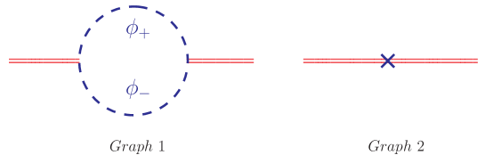
Figure 1: The one-loop and counterterm corrections to the $D^{2}$-term. The blue dotted lines in Graph 1 denote the messenger scalar fields in mass eigenstate while the cross in Graph 2 the counterterm vertex.

We begin with the 2-point function (27) which turns outs to be one loop correction to the $D$ field propagator. The graph 1 in Figure 1 is the contribution from the scalar 2-point function of the current superfield while the graph 2 is the counterterm. Using dimensional regularization the amplitude for Graph 1 is given by

$$i\Omega(p^{2}) = 2g^{2}\mathbf{C}(\mathrm{R})\mu^{2\varepsilon}\int\frac{d^{d}q}{(2\pi)^{d}}\frac{1}{(q^{2}-M^{2}_{+})[(q+p)^{2}-M^{2}_{-}]}$$

$$= \frac{2ig^{2}\mathbf{C}(\mathrm{R})}{16\pi^{2}}\bigg{\{}\frac{1}{\varepsilon}-\gamma+\log 4\pi+\int^{1}_{0}dy\log\bigg{[}\frac{\mu^{2}}{M^{2}_{0}+(1-2y)F-y(1-y)p^{2}}\bigg{]}+{\cal O}(\varepsilon)\bigg{\}},$$

where $\mu$ is the renormalization scales.  This leads to the counterterm

$$Z_{D}-1=-\frac{g^{2}\mathbf{C}(\mathrm{R})}{16\pi^{2}}\frac{2}{\varepsilon}.$$ (45)

Thus the regularized scalar 2-point function at one loop is given by

$$\Omega_{R}(p^{2}) = \frac{2g^{2}\mathbf{C}(\mathrm{R})}{16\pi^{2}}\bigg{\{}\frac{x}{\hat{p}^{2}_{0}}\log\frac{1-x}{1+x}-\frac{1}{2}\log(1-x^{2})+\log\frac{\mu^{2}}{M^{2}_{0}}+2$$

$$+\bigg{(}\frac{2x}{\hat{p}^{2}_{0}}-1\bigg{)}h\bigg{(}\frac{2x-\hat{p}^{2}_{0}}{\sqrt{4x^{2}-4\hat{p}^{2}_{0}+\hat{p}^{4}_{0}}}\bigg{)}-\bigg{(}\frac{2x}{\hat{p}^{2}_{0}}+1\bigg{)}h\bigg{(}\frac{2x+\hat{p}^{2}_{0}}{\sqrt{4x^{2}-4\hat{p}^{2}_{0}+\hat{p}^{4}_{0}}}\bigg{)}\bigg{\}},$$

where $h(z)\equiv\frac{1}{z}\tan^{-1}z$, $\hat{p}^{2}_{0}\equiv\frac{p^{2}}{M^{2}_{0}}$ and $x=\frac{F}{M^{2}_{0}}$.

Figure 2: The full expression for $D$ field renormalization. The line with double-shaded blob denotes the full amplitude for $D^{2}$, and the single-shaded blobs the amplitude for the 1PI diagrams as shown in Figure 1.

By summing a geometric series of the $D^{2}$-term and the invariant function $\Omega_{R}$, the full expression for the wavefunction renormalization constant for the $D$ field, as depicted in fig. 2, is given by

$$\frac{1}{1-\Omega_{R}}=1+\Omega_{R}+\Omega_{R}^{2}+\cdots.$$ (47)

5.2 2-point function for gauge field

We compute the vector 2-point function (30). The graphs of Figure 3 denote the messenger one-loops and their counterterm corrections to the gauge boson propagators. The graph 1 and 2 have the contributions of the ferminoic and bosonic vector 2-point functions of the current superfield, respectively. The graph 3 gives the contribution of the contact term as in eq. (43), and the graph 4 does the contribution of the counterterm which cancels ultraviolet divergences of the first three graphs, in particular logarithmic ultraviolet divergences. Summing up the first three graphs, we have the amplitude for the 1PI graphs (at one loop) as

$$i\Pi_{\mu\nu}^{[1]}(p^{2})=(p_{\mu}p_{\nu}-\eta_{\mu\nu}p^{2})i\Pi^{[1]}(p^{2}),$$ (48)

which is transverse, and the invariant function $i\Pi^{[1]}(p^{2})$ is given by

$$i\Pi^{[1]}(p^{2}) = -\frac{2}{3p^{2}}g^{2}\mathbf{C}(\mathrm{R})\mu^{2\varepsilon}\int\frac{d^{d}q}{(2\pi)^{d}}\bigg{\{}\frac{(p+q)\cdot(p+2q)}{(q^{2}-M^{2}_{+})[(p+q)^{2}-M^{2}_{-}]}+(M_{+}\to M_{-})$$ (49)

$$+\frac{4q\cdot(p+q)-8M^{2}_{0}}{(q^{2}-M^{2}_{0})[(p+q)^{2}-M^{2}_{0}]}-\frac{4}{q^{2}-M^{2}_{+}}-\frac{4}{q^{2}-M^{2}_{-}}\bigg{\}}$$

$$= \frac{2ig^{2}\mathbf{C}(\mathrm{R})}{16\pi^{2}}\bigg{\{}\bigg{(}\frac{1}{\varepsilon}-\gamma+\log 4\pi\bigg{)}+\frac{4}{9}$$

$$-\frac{1}{3}\int^{1}_{0}dy(1-y)(1-6y)\log\bigg{[}\frac{\mu^{2}}{M^{2}_{+}-y(1-y)p^{2}}\bigg{]}+(M_{+}\to M_{-})$$

$$+4\int^{1}_{0}dyy(1-y)\log\bigg{[}\frac{\mu^{2}}{M^{2}_{0}-y(1-y)p^{2}}\bigg{]}$$

$$+\frac{4M^{2}_{+}}{3p^{2}}\int^{1}_{0}dy\log[1-y(1-y)\frac{p^{2}}{M^{2}_{+}}]+(M_{+}\to M_{-})+{\cal O}(\varepsilon)\bigg{\}},$$

which leads to the counterterm

$$(Z_{v}-1)^{[1]}=-\frac{g^{2}\mathbf{C}(\mathrm{R})}{16\pi^{2}}\frac{2}{\varepsilon}.$$ (50)

We note that it is the same as that of $D$ field propagator as in (45), as expected.

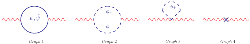
Figure 3: The one-loop and counterterm corrections to a gauge boson propagator. The blue plain lines in Graph 1 denotes the messenger fermions, the blue dotted lines in Graph 2 and 3 the messenger scalars and the cross in Graph 4 the counterterm vertex.

The regularized vector 2-point function at one loop level is given by

$$\Pi^{[1]}_{R}(p^{2}) = \frac{2g^{2}\mathbf{C}(\mathrm{R})}{16\pi^{2}}\bigg{\{}\frac{1}{6}\log\frac{\mu^{2}}{M^{2}_{+}}+\frac{1}{6}\log\frac{\mu^{2}}{M^{2}_{-}}+\frac{2}{3}\log\frac{\mu^{2}}{M^{2}_{0}}$$ (51)

$$-\frac{1}{3}\bigg{(}\frac{4}{\hat{p}^{2}_{+}}-1\bigg{)}\bigg{[}1-h\bigg{(}\sqrt{\frac{\hat{p}^{2}_{+}}{4-\hat{p}^{2}_{+}}}\bigg{)}\bigg{]}-\frac{1}{3}\bigg{(}\frac{4}{\hat{p}^{2}_{-}}-1\bigg{)}\bigg{[}1-h\bigg{(}\sqrt{\frac{\hat{p}^{2}_{-}}{4-\hat{p}^{2}_{-}}}\bigg{)}\bigg{]}$$

$$+\frac{4}{3}\bigg{(}\frac{2}{\hat{p}^{2}_{0}}+1\bigg{)}\bigg{[}1-h\bigg{(}\sqrt{\frac{\hat{p}^{2}_{0}}{4-\hat{p}^{2}_{0}}}\bigg{)}\bigg{]}\bigg{\}},$$

where $\hat{p}^{2}_{\pm}\equiv\frac{p^{2}}{M^{2}_{\pm}}$. Note that $\Pi^{[1]}_{R}(p^{2})$ goes toward $\Omega_{R}(p^{2})$ in the supersymmetric limit of $x\to 0$.

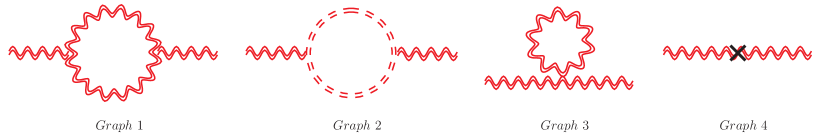
Figure 4: Additional $V$ propagator corrections: all the double lines represent superfield. Graph 1 denotes the vector loop for its own propagator, Graph 2 the ghost loop, Graph 3 the contacting vector loop, and Graph 4 the counterterm. Graph 3 vanishes in dimensional regularization.

So far we have considered the messenger fields contributions to the 2-point function for the gauge field $v^{a}_{\mu}$. In addition, there are loop contributions from its own field. Since they are totally independent of supersymmetry breaking, they are the same as those to the gaugino field. In fact, it is nothing but the contributions from the pure SuperYM theory. The graphs of fig. 4 yield these contribution to the $V$ propagator. The contribution of the gauge and gaugino field to the 2-point function for the gauge field is given by

$$i\Pi^{[2]}(p^{2})=-\frac{ig^{2}\mathbf{C}(\mathbf{G})}{16\pi^{2}}\bigg{[}\bigg{(}\frac{1}{\varepsilon}-\gamma+\log 4\pi\bigg{)}+\log\frac{\mu^{2}}{-p^{2}}+\frac{7}{3}+{\cal O}(\varepsilon)\bigg{]},$$ (52)

which leads to the counterterm

$$(Z_{v}-1)^{[2]}=\frac{g^{2}\mathbf{C}(\mathbf{G})}{16\pi^{2}}\frac{1}{\varepsilon}.$$ (53)

$$\Pi^{[2]}_{R}(p^{2})=-\frac{g^{2}\mathbf{C}(\mathbf{G})}{16\pi^{2}}\bigg{\{}\log\frac{\mu^{2}}{-p^{2}}+\frac{7}{3}\bigg{\}},$$ (54)

and then the full 2-point function for the gauge field is given by

$$\Pi_{R}(p^{2})=\Pi^{[1]}_{R}(p^{2})+\Pi^{[2]}_{R}(p^{2}).$$ (55)

By summing a geometric series of a free gauge field propagator and a vacuum polarization tensor as depicted in fig. 3 and fig. 4, the full propagator of the gauge field, as shown in fig. 5, is given by

$$\mathbf{\Delta}_{\mu\nu}(p^{2})=\frac{-i}{p^{2}[1-\Pi_{R}(p^{2})]}\bigg{(}\eta_{\mu\nu}-\frac{p_{\mu}p_{\nu}}{p^{2}}\bigg{)}+\frac{-i}{p^{2}}\bigg{(}\frac{p_{\mu}p_{\nu}}{p^{2}}\bigg{)}.$$ (56)

Its longitudinal part gets no corrections, to all orders of perturbation theory .

Figure 5: The full propagator for a gauge field. The line with the double-shaded blob on the left-hand side denotes the full propagator while the single-shaded blobs the 1PI self energies on the left-hand side.

5.3 2-point functions for gaugino field

We compute the spinor 2-point functions (29) and (30). There are two different 2-point functions for the associated with a massive gaugino field in the basis of 2-component spinors: one preserves helicity while the other changes it.

To begin with we consider a massless propagator which preserves helicity. The graph 1 of fig. 7 is the contribution of the first spinor 2-point function of the current superfield to the gaugino propagators while the graph 2 is the counterterm which cancels ultraviolet divergences of the graph 1. The amplitude for the graph 1 (at one loop) is given by

$$i\Sigma_{\alpha\dot{\alpha}}^{[1]}(p^{2})=-\sigma^{\mu}_{\alpha\dot{\alpha}}p_{\mu}i\Sigma^{[1]}(p^{2}),$$ (57)

where the invariant function $\Sigma^{[1]}(p^{2})$ is given by

$$i\Sigma^{[1]}(p^{2}) = -\frac{2}{p^{2}}g^{2}\mathbf{C}(\mathrm{R})\mu^{2\varepsilon}\int\frac{d^{d}q}{(2\pi)^{d}}\frac{1}{[(q+p)^{2}-M^{2}_{+}]}\frac{p\cdot q}{(q^{2}-M^{2}_{0})}+(M_{+}\to M_{-})$$ (58)

$$= \frac{2ig^{2}\mathbf{C}(\mathrm{R})}{16\pi^{2}}\bigg{\{}\frac{1}{\varepsilon}-\gamma+\log 4\pi+\int^{1}_{0}dxx\log\bigg{[}\frac{\mu^{2}}{M^{2}_{0}+xF-x(1-x)p^{2}}\bigg{]}$$

$$+\int^{1}_{0}dxx\log\bigg{[}\frac{\mu^{2}}{M^{2}_{0}-xF-x(1-x)p^{2}}\bigg{]}+{\cal O}(\varepsilon)\bigg{\}},$$

which leads to the counterterm

$$(Z_{\lambda}-1)^{[1]}=-\frac{g^{2}\mathbf{C}(\mathrm{R})}{16\pi^{2}}\frac{2}{\varepsilon}.$$ (59)

Once again it is the same as (45) and (50).

The regularized first spinor 2-point function is then given by

$$\Sigma^{[1]}_{R}(p^{2}) = \frac{2g^{2}\mathbf{C}(\mathrm{R})}{16\pi^{2}}\bigg{\{}-\frac{1}{2}\bigg{(}\frac{x}{\hat{p}^{2}_{0}}+1\bigg{)}^{2}h\bigg{(}\frac{x+\hat{p}^{2}_{0}}{\sqrt{(x+\hat{p}^{2}_{0})^{2}-4\hat{p}^{2}_{0}}}\bigg{)}$$

$$-\frac{1}{2}\bigg{(}\frac{x}{\hat{p}^{2}_{0}}-1\bigg{)}^{2}h\bigg{(}\frac{x-\hat{p}^{2}_{0}}{\sqrt{(x-\hat{p}^{2}_{0})^{2}-4\hat{p}^{2}_{0}}}\bigg{)}$$

$$+\frac{1}{2}\bigg{(}\frac{x^{2}}{\hat{p}^{4}_{0}}-1\bigg{)}h\bigg{(}\frac{x-\hat{p}^{2}_{0}}{\sqrt{(x+\hat{p}^{2}_{0})^{2}-4\hat{p}^{2}_{0}}}\bigg{)}+\frac{1}{2}\bigg{(}\frac{x^{2}}{\hat{p}^{4}_{0}}-1\bigg{)}h\bigg{(}\frac{x+\hat{p}^{2}_{0}}{\sqrt{(x-\hat{p}^{2}_{0})^{2}-4\hat{p}^{2}_{0}}}\bigg{)}$$

$$+2+\frac{1}{4}\bigg{(}\frac{x^{2}}{\hat{p}^{4}_{0}}-\frac{2}{\hat{p}^{2}_{0}}+1\bigg{)}\log(1-x^{2})+\frac{x}{2\hat{p}^{2}_{0}}\log\frac{1-x}{1+x}-\frac{1}{2}\log(1-x^{2})+\log\frac{\mu^{2}}{M^{2}_{0}}\bigg{\}}.$$

As expected, $\Sigma^{[1]}_{R}(p^{2})$ goes toward $\Omega_{R}(p^{2})$ in the supersymmetric limit of $x\to 0$.

There are also contributions of the gauge and gaugino fields to the gaugino propagator. Due to supersymmetry, these contributions are the same as those of gauge and gaugino fields to the gauge field propagator,

$$\Sigma^{[2]}_{R}(p^{2})=\Pi^{[2]}_{R}(p^{2}),$$ (61)

and then the full 2-point function for the massless gaugino field is given by

$$\Sigma_{R}(p^{2})=\Sigma^{[1]}_{R}(p^{2})+\Sigma^{[2]}_{R}(p^{2}).$$ (62)

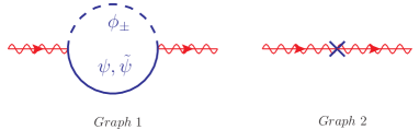
Figure 6: The one-loop and counterterm corrections to the helicity-preserving gaugino propagator. The blue plain and dotted lines in Graph 1 denote the messenger fermions and scalars, respectively, while the cross in Graph 2 the counterterm vertex.

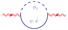
Figure 7: The one-loop contribution to the helicity-flipping gaugino propagator. The blue plain and dotted lines denote the messenger fermions and scalars, respectively.

By summing a geometric series of a massless propagator and a invariant function $\Sigma_{R}$ as depicted in fig. 4 and fig. 7, the full propagator for the massless gaugino field, as graphically shown in fig. 8, is given by

$$\frac{-i\bar{\sigma}^{\mu\dot{\alpha}\alpha}p_{\mu}}{p^{2}}\frac{1}{1-\Sigma_{R}(p^{2})}=\frac{-i\bar{\sigma}^{\mu\dot{\alpha}\alpha}p_{\mu}}{p^{2}}\big{(}1+\Sigma_{R}+\Sigma_{R}^{2}+\cdots\big{)}.$$ (63)

Figure 8: The full massless gaugino propagator in the basis of 2-component spinors. The line with the dot on the left-hand side denotes the full propagator for a massless gaugino field, and the single-shaded blobs the helicity-conserving 1PI self-energies as shown in fig. 7.

On the other hand, the graph in fig. 7 depicts the helicity changing propagator at one loop. Ultraviolet divergences of the one-loop diagrams with different internal loop fields in fig. 7 cancel by itself so that no counterterm is required. The second spinor 2-point function for the graph in fig. 7 is at 1-loop level given by $\epsilon_{\alpha\beta}i\mathcal{M}^{(1)}(p^{2})$, where

$$i{\cal M}^{(1)}(p^{2}) = -2M_{0}\frac{g^{2}\mathbf{C}(\mathrm{R})}{16\pi^{2}}\mu^{2\varepsilon}\int\frac{d^{d}q}{(2\pi)^{d}}\bigg{(}\frac{1}{q^{2}-M^{2}_{-}}-\frac{1}{q^{2}-M^{2}_{+}}\bigg{)}\frac{1}{(p+q)^{2}-M^{2}_{0}}$$ (64)

$$= -2iM_{0}\frac{g^{2}\mathbf{C}(\mathrm{R})}{16\pi^{2}}\int^{1}_{0}dy\log\bigg{[}\frac{M^{2}_{0}+(1-y)F-y(1-y)p^{2}}{M^{2}_{0}-(1-y)F-y(1-y)p^{2}}\bigg{]}$$

$$= -2iM_{0}\frac{g^{2}\mathbf{C}(\mathrm{R})}{16\pi^{2}}\bigg{\{}\frac{x}{2\hat{p}^{2}_{0}}\log(1-x^{2})-\frac{1}{2}\log\frac{1-x}{1+x}$$

$$+\bigg{(}\frac{x}{\hat{p}^{2}_{0}}-1\bigg{)}\bigg{[}h\bigg{(}\frac{x-\hat{p}^{2}_{0}}{\sqrt{(x+\hat{p}^{2}_{0})^{2}-4\hat{p}^{2}_{0}}}\bigg{)}-h\bigg{(}\frac{x-\hat{p}^{2}_{0}}{\sqrt{(x-\hat{p}^{2}_{0})^{2}-4\hat{p}^{2}_{0}}}\bigg{)}\bigg{]}$$

$$+\bigg{(}\frac{x}{\hat{p}^{2}_{0}}+1\bigg{)}\bigg{[}h\bigg{(}\frac{x+\hat{p}^{2}_{0}}{\sqrt{(x-\hat{p}^{2}_{0})^{2}-4\hat{p}^{2}_{0}}}\bigg{)}-h\bigg{(}\frac{x+\hat{p}^{2}_{0}}{\sqrt{(x+\hat{p}^{2}_{0})^{2}-4\hat{p}^{2}_{0}}}\bigg{)}\bigg{]}\bigg{\}}.$$

We note that ${\cal M}^{(1)}$ is independent of the renormalization scale $\mu$ and vanishing in the supersymmetric limit of $x\to 0$. For $p^{2}=0$, it is reduced to the well-known gaugino mass parameter as in ref. [20].

Figure 9: The full helicity-conserving propagator for the massive gaugino field. The line with double-shaded blob on the left hand side denotes the full massive gaugino propagator, and the line with black dots the full massless gaugino propagator as shown in fig. 8. The blank blobs denote the amplitude for the 1PI graphs as shown in fig. 7, and the dot-shaded blobs its complex conjugate.

We now consider two propagators for a massive gaugino field. The full helicity-preserving propagator, as graphically shown in fig. 9, is given by

$$\frac{-i\bar{\sigma}^{\mu\dot{\alpha}\alpha}p_{\mu}}{p^{2}-\frac{|\mathcal{M}|^{2}}{(1-\Sigma_{R})^{2}}}\frac{1}{1-\Sigma_{R}}=\frac{-i\bar{\sigma}^{\mu\dot{\alpha}\alpha}p_{\mu}}{p^{2}(1-\Sigma_{R})}\bigg{\{}1+\frac{|\mathcal{M}|^{2}}{p^{2}(1-\Sigma_{R})^{2}}+\bigg{[}\frac{|\mathcal{M}|^{2}}{p^{2}(1-\Sigma_{R})^{2}}\bigg{]}^{2}+\cdots\bigg{\}},$$ (65)

Figure 10: The full helicity-flipping propagator of a massive gaugino field. The line with double-shaded blob denotes the full massive gaugino propagator, and the line with black dots the full massless gaugino propagator as shown in fig. 8. The blank blobs denote the amplitude for the 1PI diagrams as shown in fig 7, and the dot-shaded blobs its complex conjugate.

while the full helicity-flipping propagator, as shown in fig. 10, is given by

$$\frac{i\frac{\mathcal{M}}{1-\Sigma_{R}}}{p^{2}-\frac{|\mathcal{M}|^{2}}{(1-\Sigma_{R})^{2}}}\frac{1}{1-\Sigma_{R}}=\frac{i\mathcal{M}}{p^{2}(1-\Sigma_{R})^{2}}\bigg{\{}1+\frac{|\mathcal{M}|^{2}}{p^{2}(1-\Sigma_{R})^{2}}+\bigg{[}\frac{|\mathcal{M}|^{2}}{p^{2}(1-\Sigma_{R})^{2}}\bigg{]}^{2}+\cdots\bigg{\}}.$$ (66)

We note that the wavefunction renormalization constants for both of the spinor propagators are the same as expected.

5.4 Supersymmetric current correlators

In the previous section we showed that $\Omega_{R}(p^{2}),\Pi^{[1]}_{R}(p^{2})$ and $\Sigma^{[1]}_{R}(p^{2})$ are, once supersymmetry is spontaneously broken ($F\neq 0$), slightly different while ${\cal M}(p^{2})$ is non-vanishing. It is noteworthy that the expressions for them are valid both for $p^{2}<F$ and for $\mu^{2}<F$, where supersymmetry is spontaneously broken. For $p^{2}>F$, supersymmetry is restored so that they are all equal and given by 

$$\Omega_{R}(p^{2})=\Pi^{[1]}_{R}(p^{2})=\Sigma^{[1]}_{R}(p^{2})=\frac{2g^{2}\mathbf{C}(\mathrm{R})}{16\pi^{2}}\bigg{[}\log\frac{\mu^{2}}{M^{2}_{0}}+2-2h\bigg{(}\sqrt{\frac{\hat{p}^{2}_{0}}{4-\hat{p}^{2}_{0}}}\bigg{)}\bigg{]},$$ (67)

while ${\cal M}(p^{2})$=0. On the other hand, the expression for $\Pi^{[2]}(p^{2})$ and $\Sigma^{[2]}(p^{2})$ is valid not only for $p^{2}<F$ but also for $p^{2}>F$.

There are also higher order correlation functions involved with the vector superfield and the renormalization of them would have to be taken into account for the complete analysis. We will perform the computations of them in the future work.

We make a comment on the scale dependence of the correlation functions. Whether or not supersymmetry is spontaneously broken in the messenger sector the coefficients of the $\log\mu$ term in the correlation functions are the same. The differences between supersymmetric and non-supersymmetric correlation functions are only from finite terms.

6 Gaugino masses

We compute the physical or renoramalized gaugino mass, which would be measured at the LHC. As previously discussed, the 1PI graph, as shown in fig. 7, gives a mass to the gaugino. No ultraviolet divergences arise from the 1PI graph, which is easily understood by comparing eq. (27) with eq. (29). For instance, ultraviolet divergences of one of the the graph, as shown in fig. 7, is cancelled by another with the minus sign, as in eq. (29). As a result, the pole mass of gaugino is finite and given by

$$\bar{m}_{\lambda}(p^{2}=\bar{m}^{2}_{\lambda},\mu)=\frac{\mathcal{M}(p^{2}=\bar{m}^{2}_{\lambda})}{1-\Sigma_{R}(p^{2}=\bar{m}^{2}_{\lambda},\mu)},$$ (68)

where ${\cal M}$ is the amplitude of the 1PI graph, and $(1-\Sigma_{R})^{-1}$ is the gaugino wavefunction renormalization constant. In order to get a physical mass we have to renormalize the gaugino wavefunction so that we get rid of the $\mu$ dependence in eq. (68). But we do not specify the renormalization procedure here .

We can now expand eq. (68) in a systematic way. To the next-to-leading order (NLO) in $\alpha(=g^{2}/4\pi)$, the physical gaugino mass is given by,

$$\bar{m}_{\lambda}(p^{2}=\bar{m}_{\lambda}^{2},\mu) \simeq \mathcal{M}^{(1)}(p^{2}=\bar{m}_{\lambda}^{2})+\mathcal{M}^{(2)}(p^{2}=\bar{m}_{\lambda}^{2})$$ (69)

$$+\mathcal{M}^{(1)}(p^{2}=\bar{m}_{\lambda}^{2})\Sigma^{(1)}_{R}(p^{2}=\bar{m}_{\lambda}^{2},\mu),$$

where ${\cal M}^{(1)}$ and $\Sigma^{(1)}_{R}$ are given by eq. (64) and (62), respectively, while $\mathcal{M}^{(2)}$ is the two-loop 1PI amplitude. Recall that the number in the superscript parenthesis stands for the order of loops. To perform the computation of complete NLO effects we would have to consider not only the two-loop 1PI amplitude $\mathcal{M}^{(2)}$ but also the one-loop gaugino wavefunction renormalization.

To complete the renormalization procedures we would have to take account of the gauge coupling renormalization as well. We sketch how to do it but the details are under current investigation [21]. The gauge coupling renormalization $Z_{g}$ is given as

$$g_{0}=Z_{g}g\mu^{\varepsilon},$$ (70)

where $g_{0}(g)$ is the bare(renormalized) coupling constant. The straightforward computation of $Z_{g}$ is through the renormalization of the gaugino-gaugino-gauge field vertex $Z_{3}$ such that

$$Z_{g}=\frac{Z_{3}}{Z_{v}^{1/2}Z_{\lambda}},$$ (71)

where $Z_{v}(Z_{\lambda})$ is the gauge(gaugino) field wavefunction renormalization. The one-loop corrections to the gaugino-gaugino-gauge field vertex is shown in fig. 11. There are two kinds of corrections to the vertex: one comes from the gaugino and gauge field loops as in the graph 1 and 2 of fig. 11 while the other from the messenger field loops as in the graph 3 and 4 of fig. 11.

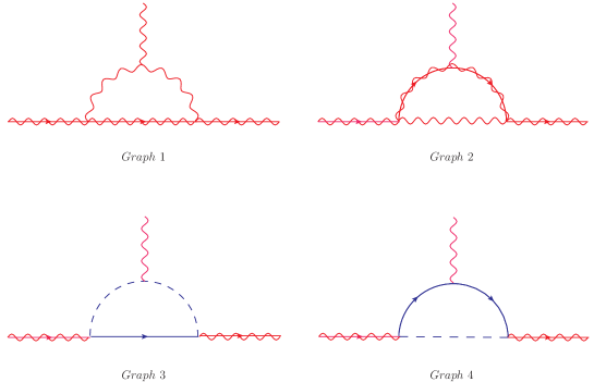
Figure 11: The one-loop corrections to the gaugino-gaugino-gauge field vertex.

7 Sfermion masses

We turn to the sfermion mass. It is protected at one loop from quadratic divergences from gauge interactions so the mass corrections begin to arise at two loop. In fact, the previous discussion about renormalization of the gaugino mass is also applied to the sfermion mass. The only difference is that the gaugino mass begins to arise at one loop while the sfermion mass at two loop. Thus the NLO effects for the sfermion mass arise at three loop.

The full propagator of a sfermion is, graphically shown in fig. 12, given by a summing of a geometric series of a massless propagator and an amplitude $-i\Xi$ for the 1PI graphs as,

Figure 12: The full propagator for a massive sfermion. The double-shaded blob represents its mass while the single-shaded blobs are 1PI graphs shown in fig. 13.

$$\frac{i}{q^{2}-\Xi(q^{2})}=\frac{i}{q^{2}}+\frac{i}{q^{2}}\frac{\Xi(q^{2})}{i}\frac{i}{q^{2}}+\frac{i}{q^{2}}\frac{\Xi(q^{2})}{i}\frac{i}{q^{2}}\frac{\Xi(q^{2})}{i}\frac{i}{q^{2}}+\cdots,$$ (72)

where $q^{\mu}$ is the four momentum of the sfermion, and $\Xi(q^{2})$ is decomposed into two parts,

$$\Xi(q^{2},\mu)=q^{2}\xi(q^{2},\mu)+\chi(\mu),$$ (73)

where $\chi$ is independent of $q^{2}$ but still depends on supersymmetry breaking parameters. As a result, the resummation of the sfermion propagators can be decomposed into the renormalized propagator and wavefunction renormalization constant,

$$\frac{i}{q^{2}-\Xi}=\frac{i}{q^{2}-\frac{\chi}{1-\xi}}\frac{1}{1-\xi},$$ (74)

where the sfermion wavefunction renormalization constant is given as $(1-\xi)^{-1}$, and the pole mass of sfermion is

$$\bar{m}^{2}_{\tilde{f}}(q^{2},\mu)=\frac{\chi(\mu)}{1-\xi(q^{2},\mu)}.$$ (75)

To the NLO in $\alpha$, the physical sfermion mass is given by

$$\bar{m}^{2}_{\tilde{f}}(q^{2}=\bar{m}^{2}_{\tilde{f}},\mu)\simeq\chi^{(2)}(\mu)+\chi^{(2)}(\mu)\xi^{(1)}(q^{2}=\bar{m}^{2}_{\tilde{f}},\mu)+\chi^{(3)}(\mu),$$ (76)

where $\chi^{(2)}$ is the well-known sfermion mass parameter as in ref. [20]. Of course, we would have to take account of renormalization as well but we will not do it in the letter.

In the context of GGM, the 1PI amplitude is given by the graphs as shown in fig. 13,

Figure 13: The 1PI graphs for a sfermion mass. The lines with double-shaded blobs stand for the full propagators for the components of the vector superfield.

$$-i\Xi(q^{2})=g^{2}\mathbf{C}(\mathrm{R})\sum_{j=1}^{4}{\cal A}_{j},$$ (77)

where

$${\cal A}_{1}(q^{2}) = \int^{F}\frac{\mathrm{d}^{4}p}{(2\pi)^{4}}\frac{1}{(p+q)^{2}}\frac{1}{1-\Omega_{R}(p^{2})},$$ (78)

$${\cal A}_{2}(q^{2}) = -4\int^{F}\frac{\mathrm{d}^{4}p}{(2\pi)^{4}}\frac{q^{2}p^{2}-(p\cdot q)^{2}}{(p^{2})^{2}(p+q)^{2}}\frac{1}{1-\Pi_{R}(p^{2})},$$ (79)

$${\cal A}_{3} = 3\int^{F}\frac{\mathrm{d}^{4}p}{(2\pi)^{4}}\frac{1}{p^{2}}\frac{1}{1-\Pi_{R}(p^{2})},$$ (80)

$${\cal A}_{4}(q^{2}) = -4\int^{F}\frac{\mathrm{d}^{4}p}{(2\pi)^{4}}\frac{p^{2}+p\cdot q}{(p+q)^{2}}\frac{1}{p^{2}-\frac{|\mathcal{M}(p^{2})|^{2}}{(1-\Sigma_{R})^{2}}}\frac{1}{1-\Sigma_{R}(p^{2})}.$$ (81)

Note that only ${\cal A}_{3}$ is independent of $q^{2}$ so that it does not contribute to the wavefunction renormalization constant of the sfermion. On the other hand, ${\cal A}_{1,2,4}$ contribute not only to the wavefunction renormalization constant of the sfermion but also to the mass of the sfermion.

Before closing this section, we would like to make a comment. As mentioned in the previous section, 3-point functions or higher order correlation functions of a vector superfield also lead to radiative corrections to the sfermion mass. These contributions can be systematically taken into account in parallel with a renormalization procedure, and will produce a result more approximate to the physical mass measured at the detectors of the LHC. Moreover, once parity conservation under $V\to-V$ is introduced, odd order correlation functions vanish so the next leading order correlation function begins at the fourth. We will pursue computation of higher order correlation functions in the future [21].

8 Summary and outlook

We revisited the GGM, in particular by taking the minimal gauge mediation as a specific example. The current superfield of an ungauged Wess-Zumino model is derived from an infinitesimal global transformation of the model. The 2-point functions of the current superfield is computed using (anti-)commutation relations among the component fields. The Fourier transformations of the scalar, first spinor and vector 2-point functions yield the vacuum polarization tensor and its two supersymmetric counterparts. Their invariant functions correspond to the wavefunction renormalization constants of the component fields of a vector superfield so we understand why these invariant functions are all the same in supersymmetric theories. For spontaneously broken supersymmetric theories, these invariant functions are all slightly different, and so do the wavefunction renormalization constants of the component fields of a vector superfield. We computed these functions at one loop using dimensional regularization.

We have shown that the physical mass of a gaugino is expressed in terms of the 1PI graphs and the wavefunction renormalization constants of the gaugino fields. The physical masses of squarks and sleptons are also expressed in terms of the wavefunction renormalization constants of the gaugino fields and the gaugino masses. Higher order correlation functions should be taken into account in order to make the effects of higher order loop of the 1PI graphs included.

The linear sigma model as an inceptive model of the GGM can be generalized to the nonlinear sigma model. In superspace notation, it implies a non-minimal Kähler potential. One can regard a non-minimal Kähler potential as an effective Kähler potential resulting from integrating out heavy superfields. In this regards, the GGM may help merge the gauge mediation with other mediation mechanisms.

9 Acknowledgements

We would like to thank Kwang Sik Jeong, Sung Jay Lee and Ann Nelson for useful comments and discussions. This research was supported by Basic Science Research Program through the National Research Foundation of Korea(NRF) funded by the Ministry of Education, Science and Technology, under contract 2010-0012779.

Appendix A Calculation of 2-point functions

In the Appendix we express four 2-point functions in terms of the current superfield as in (25). To begin with, we write down the free field 2-point functions, the propagators, which are necessary to express the 2-point functions of the current superfield:

$$\langle 0|\mbox{T}[\phi_{\pm}(x)\phi^{\ast}_{\pm}(0)]|0\rangle = i\Delta_{F}(x;M_{\pm}),$$ (82)

$$\langle 0|\mbox{T}[\psi_{\alpha}(x)\psi^{\beta}(0)]|0\rangle = \langle 0|\mbox{T}[\tilde{\psi}_{\alpha}(x)\tilde{\psi}^{\beta}(0)]|0\rangle=i\delta^{\,\,\,\beta}_{\alpha}M_{0}\Delta_{F}(x;M_{0}),$$ (83)

$$\langle 0|\mbox{T}[\bar{\psi}^{\dot{\alpha}}(x)\bar{\psi}_{\dot{\beta}}(0)]|0\rangle = \langle 0|\mbox{T}[\bar{\tilde{\psi}}^{\dot{\alpha}}(x)\bar{\tilde{\psi}}_{\dot{\beta}}(0)]|0\rangle=i\delta^{\dot{\alpha}}_{\,\,\dot{\beta}}M_{0}\Delta_{F}(x;M_{0}),$$ (84)

$$\langle 0|\mbox{T}[\psi_{\alpha}(x)\bar{\psi}_{\dot{\beta}}(0)]|0\rangle = \langle 0|\mbox{T}[\tilde{\psi}_{\alpha}(x)\bar{\tilde{\psi}}_{\dot{\beta}}(0)]|0\rangle=\sigma^{\mu}_{\alpha\dot{\beta}}\partial_{\mu}\Delta_{F}(x;M_{0}),$$ (85)

where $\Delta_{F}(x;M)$ is the propagator for a scalar field with mass $M$,

$$\Delta_{F}(x;M)\equiv\frac{1}{\Box-M^{2}}.$$ (86)

Note that there are two kinds of fermion propagators with respect to helicity: one preserves it as in eq. (85) while the other flips it as in eq. (83) and (84).

We first evaluate the scalar 2-point function of the current superfield:

$$\langle J^{a}(x)J^{a}(0)\rangle \equiv\langle 0|\mbox{T}\big{\{}J^{a}(x)J^{a}(0)\big{\}}|0\rangle$$ (87)

$$=\langle 0|\mbox{T}\big{\{}\big{(}\phi^{\dagger}_{+}T^{a}\phi_{-}(x)+\phi^{\dagger}_{-}T^{a}\phi_{+}(x)\big{)}\big{(}\phi^{\dagger}_{+}T^{a}\phi_{-}(0)+\phi^{\dagger}_{-}T^{a}\phi_{+}(0)\big{)}\big{\}}|0\rangle$$

$$=\langle 0|\mbox{T}\big{\{}\phi^{\dagger}_{+}(x)T^{a}\phi_{-}(x)\,\phi^{\dagger}_{-}(0)T^{a}\phi_{+}(0)\big{\}}|0\rangle+\langle 0|\mbox{T}\big{\{}\phi^{\dagger}_{-}(x)T^{a}\phi_{+}(x)\,\phi^{\dagger}_{+}(0)T^{a}\phi_{-}(0)\big{\}}|0\rangle$$

$$=2\langle 0|\mbox{T}\big{\{}\phi^{\ast b}_{+}(x)\phi_{+e}(0)\big{\}}|0\rangle\langle 0|\mbox{T}\big{\{}\phi^{\ast}_{-c}(x)\phi^{\,\,d}_{-}(0)\big{\}}|0\rangle T^{\boldsymbol{a}\,c}_{\,\,b}T^{\boldsymbol{a}\,e}_{\,\,d}$$

$$=2\delta^{\,\,b}_{e}i\Delta_{F}(x;M_{+})\delta^{\,\,d}_{c}i\Delta_{F}(x;M_{-})T^{\boldsymbol{a}\,c}_{\,\,b}T^{\boldsymbol{a}\,e}_{\,\,d}$$

$$=-2\mathbf{C}(\mathrm{R})\Delta_{F}(x;M_{+})\Delta_{F}(x;M_{-}),$$

where $\mathbf{C}(\mathrm{R})$ is the quadratic invariant of the fundamental representation,

$$\mbox{Tr}[T^{a}T^{b}]=\mathbf{C}(\mathrm{R})\delta^{ab}.$$ (88)

Note that (87) is symmetric under the exchange $M_{+}\leftrightarrow M_{-}$.

Next we turn to the first spinor 2-point function

$$\langle j^{a}_{\alpha}(x)\bar{j}^{a}_{\dot{\alpha}}(0)\rangle \equiv\langle 0|\mbox{T}\big{\{}j^{a}_{\alpha}(x)\bar{j}^{a}_{\dot{\alpha}}(0)\big{\}}|0\rangle$$ (89)

$$=\langle 0|\mbox{T}\big{\{}[\phi^{\dagger}_{+}(x)+\phi^{\dagger}_{-}(x)]T^{a}\psi_{\alpha}(x)\,\bar{\psi}_{\dot{\alpha}}(0)T^{a}[\phi_{+}(0)+\phi_{-}(0)]\big{\}}|0\rangle$$

$$\quad+\langle 0|\mbox{T}\big{\{}\tilde{\psi}_{\alpha}(x)T^{a}[\phi_{+}(x)-\phi_{-}(x)]\,[\phi^{\dagger}_{+}(0)-\phi^{\dagger}_{-}(0)]T^{a}\bar{\tilde{\psi}}_{\dot{\alpha}}(0)\big{\}}|0\rangle$$

$$=T^{\boldsymbol{a}\,c}_{\,\,b}T^{\boldsymbol{a}\,e}_{\,\,d}\bigg{\{}\big{[}\langle 0|\mbox{T}\big{\{}\phi^{\ast b}_{+}(x)\phi_{+e}(0)\big{\}}|0\rangle\langle 0|\mbox{T}\big{\{}\psi_{\alpha c}(x)\bar{\psi}^{d}_{\dot{\alpha}}(0)\big{\}}|0\rangle+(\phi_{+}\to\phi_{-})\big{]}$$

$$\qquad\qquad+\langle 0|\mbox{T}\big{\{}\tilde{\psi}^{b}_{\alpha}(x)\bar{\tilde{\psi}}_{\dot{\alpha}e}(0)\big{\}}|0\rangle\langle 0|\mbox{T}\big{\{}\phi_{+c}(x)\phi^{\ast d}_{+}(0)\big{\}}|0\rangle+(\phi_{+}\to\phi_{-})\big{]}\bigg{\}}$$

$$=2\mathbf{C}(\mathrm{R})\big{[}i\Delta_{F}(x;M_{+})+i\Delta_{F}(x;M_{-})\big{]}\sigma_{\alpha\dot{\alpha}}^{\mu}\partial_{\mu}\Delta_{F}(x;M_{0}).$$

Note that the first spinor 2-point function is a sum of product of one scalar and one helicity-preserving fermion propagators. Moreover, it is symmetric under the exchange $M_{+}\leftrightarrow M_{-}$.

Next we turn to the evaluation of the second spinor 2-point function

$$\langle j^{a}_{\alpha}(x)j^{a}_{\beta}(0)\rangle \equiv\langle 0|\mbox{T}\big{\{}j^{a}_{\alpha}(x)j^{a}_{\beta}(0)\big{\}}|0\rangle$$ (90)

$$=\langle 0|\mbox{T}\big{\{}[\phi^{\dagger}_{+}(x)+\phi^{\dagger}_{-}(x)]T^{a}\psi_{\alpha}(x)\,\tilde{\psi}_{\beta}(0)T^{a}[\phi_{+}(0)-\phi_{-}(0)]\big{\}}|0\rangle$$

$$\quad+\langle 0|\mbox{T}\big{\{}[\tilde{\psi}_{\alpha}(x)T^{a}[\phi_{+}(x)-\phi_{-}(x)]\,[\phi^{\dagger}_{+}(0)+\phi^{\dagger}_{-}(0)]T^{a}\psi_{\beta}(x)\big{\}}|0\rangle$$

$$=T^{\boldsymbol{a}\,c}_{\,\,b}T^{\boldsymbol{a}\,e}_{\,\,d}\bigg{\{}\big{[}\langle 0|\mbox{T}\big{\{}\phi^{\ast b}_{+}(x)\phi_{+e}(0)]\big{\}}|0\rangle-(\phi_{+}\to\phi_{-})\big{\}}|0\rangle\big{]}\langle 0|\mbox{T}\big{\{}\psi_{\alpha c}(x)\tilde{\psi}^{d}_{\beta}(0)\big{\}}|0\rangle\big{]}$$

$$\qquad\qquad\quad+\big{[}\langle 0|\mbox{T}\big{\{}\phi_{+c}(x)\phi^{\ast d}_{+}(0)\big{\}}|0\rangle-(\phi_{+}\to\phi_{-})\big{]}\langle 0|\mbox{T}\big{\{}\tilde{\psi}^{b}_{\alpha}(x)\psi_{\beta e}(0)\big{\}}|0\rangle\big{]}\bigg{\}}$$

$$=2\mathbf{C}(\mathrm{R})[\Delta_{F}(x;M_{+})-\Delta_{F}(x;M_{-})]\varepsilon_{\alpha\beta}M_{0}\Delta_{F}(x;M_{0}).$$

Note that (90) is antisymmetric not only under the exchange $M_{+}\leftrightarrow M_{-}$ but also under the exchange $\alpha\leftrightarrow\beta$.

Next we compute the bosonic vector 2-point function

$$\langle j^{aB}_{\mu}(x)j^{aB}_{\nu}(0)\rangle \equiv\langle 0|\mbox{T}\big{\{}j^{aB}_{\mu}(x)j^{aB}_{\nu}(0)\big{\}}|0\rangle$$ (91)

$$=-\langle 0|\mbox{T}\big{\{}\big{(}\phi^{\dagger}_{+}T^{a}\overleftrightarrow{\partial_{\mu}}\phi_{-}+\phi^{\dagger}_{-}T^{a}\overleftrightarrow{\partial_{\mu}}\phi_{+}\big{)}(x)\big{(}\phi^{\dagger}_{+}T^{a}\overleftrightarrow{\partial_{\nu}}\phi_{-}+\phi^{\dagger}_{-}T^{a}\overleftrightarrow{\partial_{\nu}}\phi_{+}\big{)}(0)\big{\}}|0\rangle$$

$$=-\langle 0|\mbox{T}\big{\{}\big{(}\phi^{\dagger}_{+}T^{a}\overleftrightarrow{\partial_{\mu}}\phi_{-}\big{)}(x)\big{(}\phi^{\dagger}_{-}T^{a}\overleftrightarrow{\partial_{\nu}}\phi_{+}\big{)}(0)\big{\}}|0\rangle+(\phi_{+}\leftrightarrow\phi_{-})$$

$$=2T^{\boldsymbol{a}\,c}_{\,\,b}T^{\boldsymbol{a}\,e}_{\,\,d}\big{(}\langle 0|\big{\{}\partial_{\mu}\phi^{\ast b}_{+}(x)\partial_{\nu}\phi_{+e}(0)\big{\}}|0\rangle\langle 0|\mbox{T}\big{\{}\phi_{-c}(x)\phi^{\ast d}_{-}(0)\big{\}}|0\rangle$$

$$\qquad\qquad\!\!-\langle 0|\mbox{T}\big{\{}\partial_{\mu}\phi^{\ast b}_{+}(x)\phi_{+e}(0)\big{\}}|0\rangle\langle 0|\mbox{T}\big{\{}\phi_{-c}(x)\partial_{\nu}\phi^{\ast d}_{-}(0)\big{\}}|0\rangle$$

$$\qquad\qquad\!\!+\langle 0|\mbox{T}\big{\{}\phi^{\ast b}_{+}(x)\phi_{+e}(0)\big{\}}|0\rangle\langle 0|\mbox{T}\big{\{}\partial_{\mu}\phi_{-c}(x)\partial_{\nu}\phi^{\ast d}_{-}(0)\big{\}}|0\rangle$$

$$\qquad\qquad\!\!-\langle 0|\mbox{T}\big{\{}\phi^{\ast b}_{+}(x)\partial_{\nu}\phi_{+e}(0)\big{\}}|0\rangle\langle 0|\mbox{T}\big{\{}\partial_{\mu}\phi_{-c}(x)\phi^{\ast d}_{-}(0)\big{\}}|0\rangle\big{)}$$

$$=2\mathbf{C}(\mathrm{R})\big{[}\Delta_{F}(x;M_{-})\partial_{\mu}\partial_{\nu}\Delta_{F}(x;M_{+})-\partial_{\mu}\Delta_{F}(x;M_{+})\partial_{\nu}\Delta_{F}(x;M_{-})$$

$$\qquad\qquad+\Delta_{F}(x;M_{+})\partial_{\mu}\partial_{\nu}\Delta_{F}(x;M_{-})-\partial_{\mu}\Delta_{F}(x;M_{-})\partial_{\nu}\Delta_{F}(x;M_{+})\big{]}.$$

Note that (91) is symmetric not only under the exchange $M_{+}\leftrightarrow M_{-}$ but also under the exchange $\mu\leftrightarrow\nu$.

We also compute the fermionic vector 2-point function

$$\langle j^{aF}_{\mu}(x)j^{aF}_{\nu}(0)\rangle \equiv\langle 0|\mbox{T}\big{\{}j^{aF}_{\mu}(x)j^{aF}_{\nu}(0)\big{\}}|0\rangle$$ (92)

$$=\langle 0|\mbox{T}\big{\{}\big{[}\bar{\psi}(x)\bar{\sigma}_{\mu}T^{a}\psi(x)+\tilde{\psi}(x)\sigma_{\mu}T^{a}\bar{\tilde{\psi}}(x)\big{]}\big{[}\bar{\psi}(0)\bar{\sigma}_{\nu}T^{a}\psi(0)+\tilde{\psi}(0)\sigma_{\nu}T^{a}\bar{\tilde{\psi}}(0)\big{]}\big{\}}|0\rangle$$

$$=T^{\boldsymbol{a}\,c}_{\,\,b}T^{\boldsymbol{a}\,e}_{\,\,d}\bar{\sigma}_{\mu}^{\dot{\alpha}\alpha}\bar{\sigma}_{\nu}^{\dot{\beta}\beta}\langle 0|\mbox{T}\big{\{}\bar{\psi}^{b}_{\dot{\alpha}}(x)\psi_{\beta e}(0)\big{\}}|0\rangle\langle 0|\mbox{T}\big{\{}\psi_{\alpha c}(x)\bar{\psi}^{d}_{\dot{\beta}}(0)\big{\}}|0\rangle$$

$$\,\,+T^{\boldsymbol{a}\,c}_{\,\,b}T^{\boldsymbol{a}\,e}_{\,\,d}\bar{\sigma}_{\mu}^{\dot{\alpha}\alpha}\sigma_{\nu\beta\dot{\beta}}\langle 0|\mbox{T}\big{\{}\bar{\psi}^{b}_{\dot{\alpha}}(x)\bar{\tilde{\psi}}^{\dot{\beta}}_{e}(0)\big{\}}|0\rangle\langle 0|\mbox{T}\big{\{}\psi_{\alpha c}(x)\tilde{\psi}^{\beta d}(0)\big{\}}|0\rangle$$

$$\,\,+T^{\boldsymbol{a}\,c}_{\,\,b}T^{\boldsymbol{a}\,e}_{\,\,d}\sigma_{\mu\alpha\dot{\alpha}}\bar{\sigma}_{\nu}^{\dot{\beta}\beta}\langle 0|\mbox{T}\big{\{}\tilde{\psi}^{\alpha b}(x)\psi_{\beta e}(0)\big{\}}|0\rangle\langle 0|\mbox{T}\big{\{}\bar{\tilde{\psi}}_{c}^{\dot{\alpha}}(x)\bar{\psi}^{d}_{\dot{\beta}}(0)\big{\}}|0\rangle$$

$$\,\,+T^{\boldsymbol{a}\,c}_{\,\,b}T^{\boldsymbol{a}\,e}_{\,\,d}\sigma_{\mu\alpha\dot{\alpha}}\sigma_{\nu\beta\dot{\beta}}\langle 0|\mbox{T}\big{\{}\tilde{\psi}^{\alpha b}(x)\bar{\tilde{\psi}}_{e}^{\dot{\beta}}(0)\big{\}}|0\rangle\langle 0|\mbox{T}\big{\{}\bar{\tilde{\psi}}_{c}^{\dot{\alpha}}(x)\tilde{\psi}^{\beta d}(0)\big{\}}|0\rangle$$

$$=\mathbf{C}(\mathrm{R})\bar{\sigma}_{\mu}^{\dot{\alpha}\alpha}\bar{\sigma}_{\nu}^{\dot{\beta}\beta}\sigma^{\lambda}_{\beta\dot{\alpha}}\partial_{\lambda}\Delta_{F}(x;M_{0})\sigma^{\rho}_{\alpha\dot{\beta}}\partial_{\rho}\Delta_{F}(x;M_{0})$$

$$\,\,+\mathbf{C}(\mathrm{R})\bar{\sigma}_{\mu}^{\dot{\alpha}\alpha}\sigma_{\nu\beta\dot{\beta}}\delta^{\dot{\beta}}_{\dot{\alpha}}iM_{0}\Delta_{F}(x;M_{0})\delta^{\beta}_{\alpha}iM_{0}\Delta_{F}(x;M_{0})$$

$$\,\,+\mathbf{C}(\mathrm{R})\sigma_{\mu\alpha\dot{\alpha}}\bar{\sigma}_{\nu}^{\dot{\beta}\beta}\delta^{\alpha}_{\beta}iM_{0}\Delta_{F}(x;M_{0})\delta^{\dot{\alpha}}_{\dot{\beta}}iM_{0}\Delta_{F}(x;M_{0})$$

$$\,\,+\mathbf{C}(\mathrm{R})\sigma_{\mu\alpha\dot{\alpha}}\sigma_{\nu\beta\dot{\beta}}\bar{\sigma}^{\lambda\dot{\beta}\alpha}\partial_{\lambda}\Delta_{F}(x;M_{0})\bar{\sigma}^{\rho\dot{\alpha}\beta}\partial_{\rho}\Delta_{F}(x;M_{0})$$

$$=2\mathbf{C}(\mathrm{R})\big{[}2\eta_{\mu\nu}\big{(}-\partial_{\rho}\Delta_{F}(x;M_{0})\partial^{\rho}\Delta_{F}(x;M_{0})+M_{0}^{2}\Delta^{2}_{F}(x;M_{0})\big{)}$$

$$\qquad\qquad\,\,+4\partial_{\mu}\Delta_{F}(x;M_{0})\partial_{\nu}\Delta_{F}(x;M_{0})\big{]}.$$

Note that (92) is symmetric under the exchange $\mu\leftrightarrow\nu$. The term proportional to $M_{0}^{2}$ corresponds to a product of two helicity-flipping fermion propagators while the other two terms do to a product of two helicity-conserving fermion propagators.

One looks up the Fourier transformation of these 2-point functions in ref. [10, 19].

Appendix B Loop corrections to sfermion mass

In this Appendix we compute radiative corrections to the sfermion mass as shown in fig. 13.

$$(Graph~{}1) =\int\frac{\mathrm{d}^{4}p}{(2\pi)^{4}}\frac{i}{(p+q)^{2}}(igT^{a})\frac{i}{1-\Omega(p^{2})}(igT^{a})$$ (93)

$$=g^{2}\mathbf{C}(\mathrm{R})\int\frac{\mathrm{d}^{4}p}{(2\pi)^{4}}\frac{1}{(p+q)^{2}}\frac{1}{1-\Omega(p^{2})},$$

$$(Graph~{}2) =\int\frac{\mathrm{d}^{4}p}{(2\pi)^{4}}[i(p+2q)_{\mu}gT^{a}]\frac{i}{(p+q)^{2}}[i(p+2q)_{\nu}gT^{a}]\frac{-i}{p^{2}}\frac{\eta^{\mu\nu}-p^{\mu}p^{\nu}/p^{2}}{1-\Pi(p^{2})}$$

$$=-4g^{2}\mathbf{C}(\mathrm{R})\int\frac{\mathrm{d}^{4}p}{(2\pi)^{4}}\frac{p^{2}q^{2}-(p\cdot q)^{2}}{(p^{2})^{2}(p+q)^{2}}\frac{1}{1-\Pi(p^{2})},$$

$$(Graph~{}3) =\int\frac{\mathrm{d}^{4}p}{(2\pi)^{4}}(i\eta_{\mu\nu}g^{2}T^{a}T^{a})\frac{-i}{p^{2}}\frac{\eta^{\mu\nu}-p^{\mu}p^{\nu}/p^{2}}{1-\Pi(p^{2})}$$

$$=3g^{2}\mathbf{C}(\mathrm{R})\int\frac{\mathrm{d}^{4}p}{(2\pi)^{4}}\frac{1}{p^{2}}\frac{1}{1-\Pi(p^{2})},$$

$$(Graph~{}4) =-\int\frac{\mathrm{d}^{4}p}{(2\pi)^{4}}(\sqrt{2}gT^{a})\frac{i\sigma^{\mu}_{\alpha\dot{\alpha}}(p+q)_{\mu}}{(p+q)^{2}}(-\sqrt{2}gT^{a})\frac{-i\bar{\sigma}^{\nu\dot{\alpha}\alpha}p_{\nu}}{p^{2}-\frac{|\mathcal{M}|^{2}}{(1-\Sigma(p^{2}))^{2}}}\frac{1}{1-\Sigma(p^{2})}$$

$$=-4g^{2}\mathbf{C}(\mathrm{R})\int\frac{\mathrm{d}^{4}p}{(2\pi)^{4}}\frac{p^{2}+p\cdot q}{(p+q)^{2}}\frac{1}{p^{2}-\frac{|\mathcal{M}|^{2}}{(1-\Sigma(p^{2}))^{2}}}\frac{1}{1-\Sigma(p^{2})}.$$

References

- [1] M. Dine, W. Fischler and M. Srednicki, Phys. Lett. B 104 (1981) 199.
- [2] S. Dimopoulos and S. Raby, Nucl. Phys. B 192 (1981) 353.
- [3] M. Dine and W. Fischler, Phys. Lett. B 110, 227 (1982).
- [4] C. R. Nappi and B. A. Ovrut, Phys. Lett. B 113, 175 (1982).
- [5] L. Alvarez-Gaume, M. Claudson and M. B. Wise, Nucl. Phys. B 207, 96 (1982).
- [6] S. Dimopoulos and S. Raby, Nucl. Phys. B 219, 479 (1983).
- [7] M. Dine and A. E. Nelson, Phys. Rev. D 48 (1993) 1277 [arXiv:hep-ph/9303230].
- [8] M. Dine, A. E. Nelson and Y. Shirman, Phys. Rev. D 51 (1995) 1362 [arXiv:hep-ph/9408384].
- [9] M. Dine, A. E. Nelson, Y. Nir and Y. Shirman, Phys. Rev. D 53 (1996) 2658 [arXiv:hep-ph/9507378].
- [10] P. Meade, N. Seiberg and D. Shih, Prog. Theor. Phys. Suppl. 177 (2009) 143 [arXiv:0801.3278 [hep-ph]].
- [11] M. Buican, P. Meade, N. Seiberg and D. Shih, JHEP 0903 (2009) 016 [arXiv:0812.3668 [hep-ph]].
- [12] M. Buican and Z. Komargodski, JHEP 1002 (2010) 005 [arXiv:0909.4824 [hep-ph]].
- [13] G. F. Giudice and R. Rattazzi, Nucl. Phys. B 511 (1998) 25 [arXiv:hep-ph/9706540].
- [14] N. Arkani-Hamed, G. F. Giudice, M. A. Luty and R. Rattazzi, Phys. Rev. D 58 (1998) 115005 [arXiv:hep-ph/9803290].
- [15] S. Weinberg, Cambridge, UK: Univ. Pr. (2000) 419 p
- [16] J. Wess and J. Bagger, Princeton, USA: Univ. Pr. (1992) 259 p
- [17] A. Salam and J. A. Strathdee, Fortsch. Phys. 26 (1978) 57.
- [18] J. A. de Azcarraga, J. Lukierski and P. Vindel, Czech. J. Phys. B 37 (1987) 401.
- [19] D. Marques, JHEP 0903 (2009) 038 [arXiv:0901.1326 [hep-ph]].
- [20] S. P. Martin, Phys. Rev. D 55 (1997) 3177 [arXiv:hep-ph/9608224].
- [21] in preparation.