On Ergodicity, Infinite Flow and Consensus in Random Models

Abstract

We consider the ergodicity and consensus problem for a discrete-time linear dynamic model driven by random stochastic matrices, which is equivalent to studying these concepts for the product of such matrices. Our focus is on the model where the random matrices have independent but time-variant distribution. We introduce a new phenomenon, the infinite flow, and we study its fundamental properties and relations with the ergodicity and consensus. The central result is the infinite flow theorem establishing the equivalence between the infinite flow and the ergodicity for a class of independent random models, where the matrices in the model have a common steady state in expectation and a feedback property. For such models, this result demonstrates that the expected infinite flow is both necessary and sufficient for the ergodicity. The result is providing a deterministic characterization of the ergodicity, which can be used for studying the consensus and average consensus over random graphs.

Keywords: Ergodicity, random consensus, linear random model, product of random matrices, infinite flow.

1 Introduction

There is evidence of a growing number of applications in decentralized control of networked agents, as well as social and other networks where the consensus is used as a mechanism for decentralized coordination of agent actions. The focus of this paper is on a canonical consensus problem for a linear discrete-time dynamic system driven by a general model of random matrices, where the matrices are row-stochastic. Investigating whether the model reaches a consensus or not is often done by exploring the conditions that ensure the ergodicity, which in turn always guarantees the consensus.

In this paper, we propose an alternative approach by introducing a concept of the model with infinite flow property, which can be interpreted as infinite information flow over time between a group of agents and the other agents in the network. We show that the infinite flow property is closely related to the ergodicity and, hence, to the consensus. In particular, we show the equivalence between the infinite flow and the ergodicity for a class of independent random models.

We start by a comprehensive study of the fundamental relations and properties of the ergodicity, consensus and infinite flow for general random models, independent models and independent identically distributed (i.i.d.) random models. We then investigate the random models with a feedback property and the models with a common steady state for the expected matrices. Both of these properties have been used in the analysis of consensus models, but a deeper understanding of their roles has not been observed. We classify feedback property in three basic types from weak to strong and show some relations for them. Then, we study the models with a common steady state in expectation. By putting all the pieces together, we show that the ergodicity of the model is equivalent to the infinite flow property for a class of independent random models with feedback property and a common steady state in expectation, as given in infinite flow theorem (Theorem 7). The infinite flow theorem also establishes the equivalence between the infinite flow properties of the model and the expected model. Furthermore, the theorem also shows the equivalence between the ergodicity of the model and the ergodicity of the expected model. As such, the theorem provides a novel deterministic characterization of the ergodicity, thus rendering another tool for studying the consensus over random networks and convergence of random consensus algorithms.

The main contributions of this paper include: 1) the equivalence of the ergodicity of the model and the expected model for a class of independent random models with a feedback property and a common steady state in expectation; 2) the new insights and understanding of the ergodicity and consensus events over random networks brought to light through a new phenomena of infinite flow event, which to the best of our knowledge has not been known prior to this work; 3) novel comprehensive study of the fundamental properties of the consensus and ergodicity events for general class of independent random models; 4) new insights into the role of feedback property and the role of a common steady state in expectation for the ergodicity and consensus.

The study of the random product of stochastic matrices dates back to the early work in [1] where the convergence of the product of i.i.d. random stochastic matrices was studied using the algebraic and topological structures of the set of stochastic matrices. This work was further extended in [2, 3, 4] by using results from ergodic theory of stationary processes and their algebraic properties. In [5], the ergodicity and consensus of the product of i.i.d. random stochastic matrices was studied using tools from linear algebra and probability theory, and a necessary and sufficient condition for the ergodicity was established for a class of i.i.d. models. Independently, the same problem was tackled in [6], where an exponential convergence bound was established. Recently, the work in [5] was extended to ergodic stationary processes in [7].

In all of the works [1, 2, 3, 4, 5, 6, 7], the underlying random models are assumed to be either i.i.d. or stationary processes, both of which imply time-invariant distribution on the random model. Unlike these works, our work in this paper is focused on the independent random models with time-variant distributions. Furthermore, we study ergodicity and consensus for such models using martingale and supermartingale convergence results combined with the basic tools from probability theory. Our work is also related to the consensus over random networks [8], optimization over random networks [9], and the consensus over a network with random link failures [10]. Related are also gossip and broadcast-gossip schemes giving rise to a random consensus over a given connected bi-directional communication network [11, 12, 13, 14]. On a broader basis, the paper is related to the literature on the consensus over networks with noisy links [15, 16, 17, 18] and the deterministic consensus in decentralized systems models [19, 20, 21, 22, 23], [24, 25, 26, 27] including the effects of quantization and delay [28, 29, 30, 31, 32, 14].

The paper is organized as follows. In Section 2, we describe a discrete-time random linear dynamic system of our interest, and introduce the ergodicity, consensus and infinite flow events. In Section 3, we explore the relations among these events and establish their 0-1 law and other properties by considering general, independent and i.i.d. random models. In Section 4, we discuss models with feedback properties and provide classification of such properties with insights into their relations. We also consider independent random model with a common steady state in expectation. In Section 5, we focus on independent random models with infinite flow property. We establish necessary and sufficient conditions for ergodicity, and briefly discuss some implications of these conditions. We conclude in Section 6.

Notation and Basic Terminology. We view all vectors as columns. For a vector $x$, we write $x_{i}$ to denote its $i$th entry, and we write $x\geq 0$ ($x>0$) to denote that all its entries are nonnegative (positive). We use $x^{T}$ to denote the transpose of a vector $x$. We write $\|x\|$ to denote the standard Euclidean vector norm i.e., $\|x\|=\sqrt{\sum_{i}x_{i}^{2}}$. We use $e_{i}$ to denote the vector with the $i$th entry equal to 1 and all other entries equal to $0$, and use $e$ to denote the vector with all entries equal to $1$. A vector $a$ is stochastic when $a\geq 0$ and $\sum_{i}a_{i}=1$. We write $\{x(k)\}$ or $\{x(k)\}_{k\geq 0}$ to denote a sequence $x(0),x(1),\ldots$ of some elements, and we write $\{x(k)\}_{k\geq t}$ to denote the truncated sequence $x(t),x(t+1),\ldots$ for $t>0$. For a set $C$ and a subset $S$ of $C$, we write $S\subset C$ to denote that $S$ is a proper subset of $C$. A set $S\subset C$ such that $S\neq\emptyset$ is referred to as a nontrivial subset of $C$. We write $[m]$ to denote the integer set $\{1,\ldots,m\}$. For a set $S\subset[m]$, we let $\bar{S}$ denote the complement set of $S$ with respect to $[m]$, i.e., $\bar{S}=\{i\in[m]\mid i\notin S\}$.

We denote the identity matrix by $I$. For a vector $v$, we use $diag(v)$ to denote the diagonal matrix with diagonal entries being the components $v_{i}$ of the vector $v$. For a matrix $W$, we write $W_{ij}$ to denote its $(i,j)$th entry, $W^{i}$ to denote its $i$th column vector, and $W^{T}$ to denote its transpose. For an $m\times m$ matrix $W$, we use $\sum_{i<j}W_{ij}$ to denote the summation of the entries $W_{ij}$ over all $i,j\in[m]$ with $i<j$. A matrix $W$ is row-stochastic when its entries are nonnegative and $We=e$. Since we deal exclusively with row-stochastic matrices, we will refer to such matrices simply as stochastic. We let $\mathbb{S}^{m}$ denote the set of $m\times m$ stochastic matrices. A matrix $W$ is doubly stochastic when both $W$ and $W^{T}$ are stochastic.

We write $\mathsf{E}\!\left[X\right]$ to denote the expected value of a random variable $X$. We use $\mathsf{Pr}(\mathscr{A})$ and ${\it 1}_{\mathscr{A}}$ to denote the probability and the characteristic function of an event $\mathscr{A}$, respectively. If $\mathsf{Pr}(\mathscr{A})=1$, we say that $\mathscr{A}$ happens almost surely. We often abbreviate “almost surely” by a.s.

2 Problem Formulation and Terminology

Throughout this article, we deal exclusively with the matrices in the set $\mathbb{S}^{m}$ of $m\times m$ stochastic matrices. We consider the topology induced by the open sets in $\mathbb{S}^{m}$ with respect to the Euclidean norm and the Borel sigma-algebra $\mathscr{F}_{\mathbb{S}^{m}}$ of this topology. We assume that we are given a probability space $(\Omega,\mathscr{R},\mathsf{Pr}(\cdot))$ and a measurable function $W:\Omega\to\Pi_{k=0}^{\infty}\,\mathbb{S}^{m}$. To every $\omega\in\Omega$, the function $W(\cdot)$ is assigning a discrete time process $\{W(k)\}(\omega)$ in the countable product measurable space $\Pi_{k=0}^{\infty}\,(\mathbb{S}^{m},\mathscr{F}_{\mathbb{S}^{m}})$, where $W(k)\in\mathbb{S}^{m}$ is the random matrix of the process at time $k$. We refer to the process $\{W(k)\}(\omega)$ interchangeably as a random chain or a random model and, when suitable, we suppress the explicit dependence on the variable $\omega$. We say that the chain $\{W(k)\}$ is independent if the sigma algebras generated by the $W(k)$s for different $k\geq 0$ are independent. If in addition $W(k)$s are identically distributed, then the model is independent identically distributed (i.i.d.).

With a given random chain $\{W(k)\}$, we associate a linear discrete-time dynamic system of the following form:

$$x(k+1)=W(k)x(k)\qquad\hbox{for $k=0,1,2,\ldots$},$$ (1)

where $x(k)\in\mathbb{R}^{m}$ is a state vector at time $k$ and $x(0)$ is the initial state vector. We will often refer to the system in (1) as the dynamic system driven by the chain $\{W(k)\}$.

We are interested in providing conditions guaranteeing that the dynamic system reaches a consensus almost surely. Since reaching the consensus is closely related to the ergodicity of the chain, we are also interested in studying the ergodicity on the fundamental level. In our study of the random consensus and ergodicity, we use another property of the chain, an infinite flow property. We start by providing these basic notions for a deterministic chain.

Definition 1.

Given a deterministic chain $\{G(k)\}\subset\mathbb{S}^{m}$, we say that:
The system $z(k+1)=G(k)z(k)$ reaches a consensus if for any initial state $z(0)\in\mathbb{R}^{m}$, there exists a scalar $c(z(0))$ such that $\lim_{k\to\infty}\|z(k)-c(z(0))\,e\|=0.$
The chain $\{G(k)\}$ is ergodic if for any $t\geq 0$ and $j\in[m]$, there is a scalar $g_{j}(t)$ such that

$$\lim_{k\rightarrow\infty}\Phi_{ij}(k,t)=g_{j}(t)\qquad\hbox{for all $i\in[m]$},$$

where $\Phi(k,t)=G(k)G(k-1)\cdots G(t)$ for $k>t$ and $t\geq 0$.
The chain $\{G(k)\}$ has infinite flow property if $\sum_{k=0}^{\infty}\sum_{i\in S,\,j\in\bar{S}}\left(G_{ij}(k)+G_{ji}(k)\right)=\infty$ for any nontrivial subset $S\subset[m]$.

In the definition of the infinite flow property, the quantity $\sum_{i\in S,\,j\in\bar{S}}\left(G_{ij}(k)+G_{ji}(k)\right)$ can be interpreted as a flow between the subset $S$ and its complement $\bar{S}$ in a weighted graph. In particular, consider the undirected weighted graph $\mathcal{G}(k)$ with the node set $[m]$, the edge set induced by the positive entries in $G(k)+G^{T}(k)$, and the weight matrix $G(k)+G^{T}(k)$. Then, the quantity $\sum_{i\in S,\,j\in\bar{S}}\left(G_{ij}(k)+G_{ji}(k)\right)$ represents the flow in graph $\mathcal{G}(k)$ across the cut $(S,\bar{S})$ for a nontrivial node set $S\subset[m]$ and its complement $\bar{S}$. For the graphs $\mathcal{G}(k)$ induced by the matrices $G(k)$, the infinite flow property requires that the total flow in time across any nontrivial cut $(S,\bar{S})$ is infinite, which could be viewed as infinite information exchange between the nodes in $S$ and $\bar{S}$.

The ergodicity is equivalent to the following condition [33]: for any $t\geq 0$ and $x\in\mathbb{R}^{m}$, there is a scalar $\gamma(t,x)$ such that $\lim_{k\rightarrow\infty}\Phi(k,t)x=\gamma(t,x)\,e.$ Since the matrices $G(k)$ have finite dimension, the ergodicity is also equivalent to the following condition: for any $t\geq 0$ and any $\ell\in[m]$, there is a scalar $\gamma_{\ell}(t)$ such that $\lim_{k\rightarrow\infty}\Phi(k,t)e_{\ell}=\gamma_{\ell}(t)\,e.$ Also, due to the linearity and finite dimension of the system $z(k+1)=G(k)z(k)$, the consensus can be studied by considering only the initial states $x(0)=e_{\ell}$, $\ell\in[m]$, rather than all $x(0)\in\mathbb{R}^{m}$.

Clearly, the ergodicity of the chain implies reaching a consensus. However, a consensus may be reached even if the chain $\{G(k)\}$ is not ergodic, as seen in the following example.

Example 1.

Let $G(0)=ev^{T}$ for a stochastic vector $v$, and let $G(k)=I$ for all $k\geq 1$. Then, we have $\Phi(k,0)=ev^{T}$ for all $k\geq 1,$ implying that the system $x(k+1)=G(k)x(k)$ reaches a consensus. However, the chain $\{G(k)\}$ is not ergodic since $\Phi(k,t)=I$ for any $k>t\geq 1$. $\square$

Using Definition 1, we now introduce the corresponding events of consensus, ergodicity and infinite flow. Given a random chain $\{W(k)\}$, let $\mathscr{C}$ denote the event that the system in (1) reaches a consensus for any initial state $x(0)$. Let $\mathscr{E}$ denote the event that the chain $\{W(k)\}$ is ergodic, and let $\mathscr{F}$ denote the event that the chain has the infinite flow property. We refer to $\mathscr{C}$, $\mathscr{E}$ and $\mathscr{F}$ as the consensus event, the ergodicity event and the infinite flow event, respectively. We say that the model is ergodic if the ergodicity event $\mathscr{E}$ occurs almost surely. The model admits consensus if the consensus event $\mathscr{C}$ occurs almost surely. The model has infinite flow if the infinite flow event $\mathscr{F}$ occurs almost surely. The model has expected infinite flow if its expected chain $\{\mathsf{E}\!\left[W(k)\right]\}$ has infinite flow.

3 Infinite Flow, Ergodicity and Consensus

In this section, we further study the ergodicity event $\mathscr{E}$, the consensus event $\mathscr{C}$ and the infinite flow event $\mathscr{F}$ under different assumptions on the nature of the randomness in the model. In particular, in Section 3.1 we establish some fundamental relations among $\mathscr{E}$, $\mathscr{C}$ and $\mathscr{F}$. In Section 3.2, we investigate the 0-1 law properties of these events, while in Section 3.3 we provide some relations for a random model and its expected model.

Throughout the rest of the paper, we use the following notation. For a stochastic matrix $W$ and a nontrivial subset $S\subset[m]$, we define $W_{S}$ as follows:

$$W_{S}=\sum_{i\in S,j\in\bar{S}}\left(W_{ij}+W_{ji}\right).$$ (2)

Note that for a given a random model $\{W(k)\}$, the infinite flow event $\mathscr{F}$ is given by

$$\mathscr{F}=\bigcap_{S\subset[m]}\left\{\sum_{k=0}^{\infty}W_{S}(k)=\infty\right\}.$$ (3)

Note also that the infinite flow event requires that, across any nontrivial cut $(S,\bar{S})$, the total flow in the random graphs induced by the matrices $W(k)+W^{T}(k),k\geq 0,$ is infinite.

3.1 Basic Relations

As discussed in Section 2, we have $\mathscr{E}\subseteq\mathscr{C}$ for any random model. We here show that the ergodicity event is also always contained in the infinite flow event, i.e., $\mathscr{E}\subseteq\mathscr{F}$. We establish this by using the following result for a deterministic model.

Lemma 1.

Let $\{A(k)\}\subset\mathbb{S}^{m}$ be a deterministic sequence, and let $\{z(k)\}$ be generated by $z(k+1)=A(k)z(k)$ for all $k\geq 0$ with an initial state $z(0)\in\mathbb{R}^{m}$. Then, for any nontrivial subset $S\subset[m]$ and $k\geq 0$, we have

$$\max_{i\in S}z_{i}(k+1)\leq\max_{s\in S}z_{s}(0)+d(z(0))\,\sum_{t=0}^{k}A_{S}(t),$$

$$\min_{j\in\bar{S}}z_{j}(k+1)\geq\min_{r\in\bar{S}}z_{r}(0)-d(z(0))\,\sum_{t=0}^{k}A_{S}(t),$$

where $d(y)=\max_{\ell\in[m]}y_{\ell}-\min_{r\in[m]}y_{r}$ for $y\in\mathbb{R}^{m}.$

Proof.

Let $S\subset[m]$ be an arbitrary nontrivial set and let $k\geq 0$ be arbitrary. Let $z_{\min}(k)=\min_{r\in[m]}z_{r}$ and $z_{\max}(k)=\max_{s\in[m]}z_{s}(k)$. Since $z_{i}(k+1)=\sum_{\ell=1}^{m}A_{i\ell}(k)z_{\ell}(k)$, by the stochasticity of $A(k)$ we have $z_{i}(k)\in[z_{\min}(0),z_{\max}(0)]$ for all $i\in[m]$ and all $k$. Then, we obtain for $i\in S$,

$$z_{i}(k+1)=\sum_{\ell\in S}A_{i\ell}(k)z_{\ell}(k)+\sum_{\ell\in\bar{S}}A_{i\ell}(k)z_{\ell}(k)$$

$$\quad\leq\sum_{\ell\in S}A_{i\ell}(k)\left(\max_{s\in S}z_{s}(k)\right)+z_{\max}(0)\sum_{\ell\in\bar{S}}A_{i\ell}(k),$$ (4)

where the inequality follows by $A_{i\ell}(k)\geq 0$. By the stochasticity of $A(k)$, we also obtain

$$z_{i}(k+1)\leq\left(1-\sum_{\ell\in\bar{S}}A_{i\ell}(k)\right)\max_{s\in S}z_{s}(k)$$

$$\qquad\qquad+z_{\max}(0)\sum_{\ell\in\bar{S}}A_{i\ell}(k)$$

$$=\max_{s\in S}z_{s}(k)+\left(z_{\max}(0)-\max_{s\in S}z_{s}(k)\right)\sum_{\ell\in\bar{S}}A_{i\ell}(k).$$

By the definition of $A_{S}$ in (2), we have $0\leq\sum_{\ell\in\bar{S}}A_{i\ell}(k)\leq A_{S}(k)$. Since $z_{\max}(0)-\max_{s\in S}z_{s}(k)\geq 0$, it follows

$$z_{i}(k+1) \leq\max_{s\in S}z_{s}(k)+(z_{\max}(0)-\max_{s\in S}z_{s}(k))A_{S}(k)$$

$$\leq\max_{s\in S}z_{s}(k)+d(z(0))A_{S}(k),$$

where the last inequality holds since $z_{\max}(0)-\max_{s\in S}z_{s}(k)\leq z_{\max}(0)-z_{\min}(0)=d(z(0))$. By taking the maximum over all $i\in S$ in the preceding relation and by recursively using the resulting inequality, we obtain $\max_{i\in S}z_{i}(k+1)\leq\max_{s\in S}z_{s}(k)+d(z(0))A_{S}(k)$ and recursively, we get $\max_{i\in S}z_{i}(k+1)\leq\max_{s\in S}z_{s}(0)+d(z(0))\sum_{t=0}^{k}A_{S}(t)$.

The relation for $\min_{j\in\bar{S}}z(k+1)$ follows from the preceding relation by considering $\{z(k)\}$ generated with the starting point $-z(0)$.  Q.E.D.

Using Lemma 1, we now show that the ergodicity event is contained in the infinite flow event.

Theorem 1.

Let $\{A(k)\}\subset\mathbb{S}^{m}$ be an ergodic deterministic chain. Then $\sum_{k=0}^{\infty}A_{S}(k)=\infty$ for any nontrivial $S\subset[m]$. In particular, we have $\mathscr{E}\subseteq\mathscr{F}$ for any random model.

Proof.

To arrive at a contradiction, assume that there is a nontrivial set $S\subset[m]$ such that $\sum_{k=0}^{\infty}A_{S}(k)<\infty$. Since the matrices $A(k)$ are stochastic, we have $A_{S}(k)\geq 0$ for all $k$. Therefore, there exists large enough $\bar{t}\geq 0$ such that $\sum_{k=\bar{t}}^{\infty}A_{S}(k)<\frac{1}{4}$.

Now, define the vector $\bar{z}=(\bar{z}_{1},\ldots,\bar{z}_{m})^{T}$, where $\bar{z}_{i}=0$ for $i\in S$ and $\bar{z}_{i}=1$ for $i\in\bar{S}$. Consider the dynamic system $z(k+1)=A(k)z(k)$ for $k\geq\bar{t}$, which is started at time $\bar{t}$ in state $z(\bar{t})=\bar{z}$. Note that Lemma 1 applies to the case where the time $t=\bar{t}$ is taken as initial time, in which case $d(0)$ corresponds to $d(\bar{t})=\max_{i}z_{i}(\bar{t})-\min_{j}z_{j}(\bar{t})$. Also, note that $d(\bar{t})=1$ by the definition of the starting state $\bar{z}$. Thus, by applying Lemma 1, we have for all $k\geq\bar{t}$, $\max_{i\in S}z_{i}(k+1)\leq\max_{s\in S}z_{s}(\bar{t})+\sum_{t=\bar{t}}^{k}A_{S}(t)$ and $\min_{j\in\bar{S}}z_{j}(k+1)\geq\min_{r\in\bar{S}}z_{r}(\bar{t})-\sum_{t=\bar{t}}^{k}A_{S}(t)$. Since $\max_{s\in S}z_{s}(\bar{t})=0$ and $\min_{r\in\bar{S}}z_{r}(\bar{t})=1$, it follows that $\max_{i\in S}z_{i}(k+1)\leq\sum_{t=\bar{t}}^{k}A_{S}(t)$ and $\min_{j\in\bar{S}}z_{j}(k+1)\geq 1-\sum_{t=\bar{t}}^{k}A_{S}(t)$. Using these relations and $\sum_{k=\bar{t}}^{\infty}A_{S}(k)<\frac{1}{4}$, we have $\liminf_{k\rightarrow\infty}\left(z_{j}(k)-z_{i}(k)\right)>1-2\sum_{t=\bar{t}}^{\infty}A_{S}(t)=\frac{1}{2}$ for any $j\in\bar{S}$ and $i\in S$, thus showing that the chain $\{A(k)\}$ is not ergodic - a contradiction. Therefore, we must have $\sum_{t=0}^{\infty}A_{S}(t)=\infty$ for any nontrivial $S\subset[m]$.

From the preceding argument and the definitions of $\mathscr{E}$ and $\mathscr{F}$, we conclude that $\omega\in\mathscr{E}$ implies $\omega\in\mathscr{F}$ for any random model $\{W(k)\}$. Hence, $\mathscr{E}\subseteq\mathscr{F}$ for any random model.  Q.E.D.

Theorem 1 shows that an ergodic model must have an infinite flow property. In other words, the infinite flow property of any random model is necessary for the ergodicity of the model. Later in Theorem 6, for a certain class of random models, we will show that the infinite flow is also sufficient for the ergodicity.

Figure 1 illustrates the inclusions $\mathscr{E}\subseteq\mathscr{C}$ and $\mathscr{E}\subseteq\mathscr{F}$ for a general random model. The inclusion $\mathscr{E}\subseteq\mathscr{C}\cap\mathscr{F}$ in Figure 1 can be strict as seen in the following example.

Example 2.

Consider the $2\times 2$ chain $\{A(k)\}$ defined by

$$A(0)=\left[\begin{array}[]{cc}\frac{1}{2}&\frac{1}{2}\\ \frac{1}{2}&\frac{1}{2}\end{array}\right],\ \hbox{ and }\ A(k)=\left[\begin{array}[]{cc}0&1\\ 1&0\end{array}\right]\ \hbox{for $k\geq 1$}.$$

For any stochastic matrix $B$, we have $BA(0)=A(0)$ and hence, the model admits consensus. Furthermore, the model has infinite flow property. However, the chain $\{A(k)\}_{k\geq 1}$ does not admit consensus. Therefore, in this case $\mathscr{C}\cap\mathscr{F}=\Omega$ (the entire space of realizations) while $\mathscr{E}=\emptyset$. $\square$

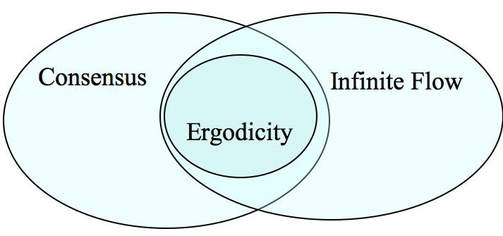
Figure 1: The relations among the ergodicity, consensus, and infinite flow events for a general random model.

Next, we provide a sufficient condition for the ergodicity and consensus events to coincide.

Lemma 2.

Let $\{W(k)\}$ be a (not necessarily independent) random chain such that each matrix $W(k)$ is invertible almost surely. Then, we have $\mathscr{E}=\mathscr{C}$ almost surely.

Proof.

The inclusion $\mathscr{E}\subseteq\mathscr{C}$ follows from the definition, so it suffices to show $\mathscr{C}\subseteq\mathscr{E}$ almost surely. In turn, to show $\mathscr{C}\subseteq\mathscr{E}$ almost surely, it suffices to prove that $\mathscr{C}\cap R\subseteq\mathscr{E}$ for a set $R$ such that $\mathsf{Pr}(R)=1$. For each $k\geq 0$, let $R_{k}$ be the set of instances $\omega$ such that the matrix $W(k)(\omega)$ is invertible. Define $R=\cap_{k=0}^{\infty}R_{k}$. We have $\mathsf{Pr}(R_{k})=1$ for each $k\geq 0$ by our assumption that each matrix $W(k)$ is invertible almost surely. In view of this and the fact that the collection $\{R_{k}\}$ is countable, it follows that $\mathsf{Pr}(R)=1$.

We next show that $\mathscr{C}\cap R\subseteq\mathscr{E}$. Let $\omega\in\mathscr{C}\cap R$ so that $W(k)(\omega)$ has full rank for all $k\geq 0$. To simplify notation, let $\tilde{W}(k)=W(k)(\omega)$. Consider an arbitrary starting time $s\geq 0$. We show that the consensus is reached for the dynamic $z(t)=\tilde{W}(t-1)z(t-1)$ with $t>s$, i.e., for any $z(s)\in\mathbb{R}^{m}$, we have $\lim_{t\rightarrow\infty}z(t)=ce$ for some $c\in\mathbb{R}$. For a given $z(s)\in\mathbb{R}^{m}$, define $\tilde{x}(0)=[\tilde{W}(s-1)\cdots\tilde{W}(1)\tilde{W}(0)]^{-1}z(s)$ and consider the dynamic $\tilde{x}(k)=\tilde{W}(k-1)\tilde{x}(k-1)$ started at time $t_{0}=0$ with the initial vector $\tilde{x}(0)$. By the definition of $\tilde{x}(0)$, we have $\tilde{x}(s)=\tilde{W}(s-1)\cdots\tilde{W}(1)\tilde{W}(0)\tilde{x}(0)=z(s)$. Therefore, for all $t>s$,

$$\tilde{x}(t) =\tilde{W}(t-1)\cdots\tilde{W}(s-1)\cdots\tilde{W}(1)\tilde{W}(0)\tilde{x}(0)$$

$$=\tilde{W}(t-1)\cdots\tilde{W}(s)z(s)=z(t).$$

By the definition of $\tilde{W}(k)$, we have $\lim_{t\rightarrow\infty}\tilde{x}(t)=ce$ for some $c\in\mathbb{R}$ (since $\omega\in\mathscr{C}$). Therefore, it follows that $\lim_{t\rightarrow\infty}z(t)=ce$, thus showing that the dynamic system $z(t)=\tilde{W}(t-1)z(t-1)$, $t>s,$ reaches a consensus. Since this is true for arbitrary $s\geq 0$ and $z(s)\in\mathbb{R}^{m}$, the chain $\{W(k)\}(\omega)$ is ergodic, which implies $\omega\in\mathscr{E}$.  Q.E.D.

In general, there may be no further refinements of inclusion relations among the events $\mathscr{E},\mathscr{F}$ and $\mathscr{C}$ even when the model is independent, as indicated by the following example.

Example 3.

Consider an independent random model where for $p\in(0,1]$, we have $W(0)=\frac{1}{m}ee^{T}$ with probability $p$, $W(0)=I$ with probability $1-p$s and $W(k)=I$ with probability $1$ for all $k\geq 1.$ In this case, the consensus event $\mathscr{C}$ happens with probability $p>0$. However, the infinite flow and the ergodicity events are empty sets. $\square$

Example 3 shows that we can have $\mathscr{C}\cap\mathscr{E}=\emptyset$ and $\mathscr{C}\cap\mathscr{F}=\emptyset$, while $\mathscr{C}\neq\emptyset$. Thus, even for an independent model the consensus event need not be contained in either $\mathscr{E}$ or $\mathscr{F}$. However, if we further restrict our attention to i.i.d. models, we can show that $\mathscr{E}=\mathscr{C}$ almost surely. To establish this, we make use of the following lemma.

Lemma 3.

Let $A\in\mathbb{S}^{m}$ and $x\in\mathbb{R}^{m}$. Also, let $A$ be such that $\max_{i\in[m]}[Ae_{\ell}]_{i}-\min_{j\in[m]}[Ae_{\ell}]_{j}\leq\frac{1}{2m}$ for any $\ell\in[m]$, where $[v]_{i}$ denotes the $i$th component of a vector $v$. Then, we have $\max_{i}[Ax]_{i}-\min_{j}[Ax]_{j}\leq\frac{1}{2}$ for any $x\in[0,1]^{m}$.

Proof.

Let $x\in\mathbb{R}^{m}$ with $x_{\ell}\in[0,1]$ for any $\ell\in[m]$. Then, we have for any $i,j\in[m]$,

$$y_{i}-y_{j} =\sum_{\ell=1}^{m}(A_{i\ell}-A_{j\ell})x_{\ell}\leq\sum_{\ell=1}^{m}|A_{i\ell}-A_{j\ell}|$$

$$=\sum_{\ell=1}^{m}\left|[Ae_{\ell}]_{i}-[Ae_{\ell}]_{j}\right|.$$

By the assumption on $A$, we obtain $\left|[Ae_{\ell}]_{i}-[Ae_{\ell}]_{j}\right|\leq\max_{i\in[m]}[Ae_{\ell}]_{i}-\min_{j\in[m]}[Ae_{\ell}]_{j}\leq\frac{1}{2m}$. Hence, $y_{i}-y_{j}\leq\sum_{\ell=1}^{m}\frac{1}{2m}=\frac{1}{2}$, implying $\max_{i}y_{i}-\min_{j}y_{j}\leq\frac{1}{2}$.  Q.E.D.

We now provide our main result for i.i.d. models, which states that the ergodicity and the consensus events are almost surely equal. We establish this result by using Lemma 3 and the Borel-Cantelli lemma (see [34], page 50).

Theorem 2.

We have $\mathscr{E}=\mathscr{C}$ almost surely for any i.i.d. random model.

Proof.

Since $\mathscr{E}\subseteq\mathscr{C}$, the assertion is true when consensus occurs with probability $0$. Therefore, it suffices to show that if the consensus occurs with a probability $p$ other than 0, the two events are almost surely equal. Let $\mathsf{Pr}(\mathscr{C})=p$ with $p\in(0,1]$. Then, for all $\omega\in\mathscr{C}$,

$$\lim_{k\to\infty}d(x(k))(\omega)=0\quad\hbox{where \ }d(x)=\max_{i}x_{i}-\min_{j}x_{j},$$

and $\{x(k)\}(\omega)$ is the sequence generated by the dynamic system (1) with any $x(0)\in\mathbb{R}^{m}$.

For every $\ell\in[m]$, let $\{x^{\ell}(k)\}$ be the sequence generated by the dynamic system in (1) with $x(0)=e_{\ell}$. Then, for any $\omega\in\mathscr{C}$, there is the smallest integer $K^{\ell}(\omega)\geq 0$ such that

$$d(x^{\ell}(k))(\omega)\leq\frac{1}{2m}\qquad\hbox{for all }k\geq K^{\ell}(\omega).$$

Note that $d(x^{\ell}(k))(\omega)$ is a nonincreasing sequence (of $k$) for each $\ell\in[m]$. Hence, by letting $K(\omega)=\max_{\ell\in[m]}K^{\ell}(\omega)$ we obtain $d(x^{\ell}(k))(\omega)\leq\frac{1}{2m}$ for all $\ell\in[m]$ and $k\geq K(\omega)$. Thus, by applying Lemma 3, we have for almost all $\omega\in\mathscr{C}$,

$$d(x(k))(\omega)\leq\frac{1}{2},$$ (5)

for all $k\geq K(\omega)$ and $x(0)\in[0,1]^{m}$. By the definition of consensus, we have $\lim_{N\to\infty}\mathsf{Pr}(K\leq N)\geq\mathsf{Pr}(\mathscr{C})=p$. Thus, by the continuity of the measure, there exists an integer $N_{1}$ such that $\mathsf{Pr}(K<N_{1})\geq\frac{p}{2}.$

Now, let time $T\geq 0$ be arbitrary, and let $l_{k}^{T}$ denote the $N_{1}$-tuple of the matrices $W(s)$ driving the system (1) for $s=T+N_{1}k,\ldots,T+N_{1}(k+1)-1$ and $k\geq 0$, i.e.,

$$l^{T}_{k} =\Bigl{(}W(T+N_{1}k),W(T+N_{1}k+1),$$

$$\qquad\ldots,W(T+N_{1}(k+1)-1)\Bigr{)}\quad\hbox{for all $k\geq 0$}.$$

Let $L_{N}$ denote the collection of all $N$-tuples $(A_{1},\ldots,A_{N})$ of matrices $A_{i}\in\mathbb{S}^{m}$, $i\in[N]$ such that for $x(N)=A_{N}A_{N-1}\cdots A_{1}x(0)$ with $x(0)\in[0,1]^{m}$, we have $d(x(N))\leq\frac{1}{2}.$ By the definitions of $l^{T}_{k}$ and $L_{N}$, relation (5) and relation $\mathsf{Pr}(K<N_{1})\geq\frac{p}{2}$ state that $\mathsf{Pr}(\{l^{T}_{0}\in L_{N_{1}}\})\geq\frac{p}{2}.$ By the i.i.d. property of the model, the events $\{l^{T}_{k}\in L_{N_{1}}\}$, $k\geq 0$, are i.i.d. and the probability of their occurrence is equal to $\mathsf{Pr}(\{l^{T}_{0}\in L_{N_{1}}\})$, implying that $\mathsf{Pr}(\{l^{T}_{k}\in L_{N_{1}}\})\geq\frac{p}{2}$ for all $k\geq 0$. Consequently, $\sum_{k=0}^{\infty}\mathsf{Pr}(\{l^{T}_{k}\in L_{N_{1}}\})=\infty.$ Since the events $\{l^{T}_{k}\in L_{N_{1}}\}$ are i.i.d., by Borel-Cantelli lemma $\mathsf{Pr}(\{\omega\in\Omega\mid\omega\in\{l^{T}_{k}\in L_{N_{1}}\}\ i.o.\})=1,$ where $i.o.$ stands for infinitely often. Observing that the event $\{\omega\in\Omega\mid\omega\in\{l^{T}_{k}\in L_{N_{1}}\}\ i.o.\}$ is contained in the consensus event for the chain $\{W(T+k)\}_{k\geq 0}$, we see that the consensus event for the chain $\{W(T+k)\}_{k\geq 0}$ occurs almost surely. Since this is true for arbitrary $T\geq 0$ it follows that the chain $\{W(k)\}$ is ergodic a.s., implying $\mathscr{C}\subseteq\mathscr{E}$ a.s. This and the inclusion $\mathscr{E}\subseteq\mathscr{C}$ yield $\mathscr{C}=\mathscr{E}$ a.s.  Q.E.D.

Theorem 2 extends the equivalence result between the consensus and ergodicity for i.i.d. models given in Theorem 3.a and Theorem 3.b of [5] (and hence Corollary 4 in [5]), which are established there assuming that the matrices have positive diagonal entries almost surely. The relations among $\mathscr{C}$, $\mathscr{E}$, and $\mathscr{F}$ for i.i.d. case are illustrated in Figure 2.

3.2 0-1 Laws

In this section, we discuss 0-1 laws for the events $\mathscr{E}$, $\mathscr{F}$ and $\mathscr{C}$ for independent random models. The 0-1 laws specify the trivial (or 0-1) events, which are the events occurring with either probability 0 or 1. The ergodicity event is a 0-1 event, as shown in [5], Lemma 1. Since the ergodicity event is always contained in the consensus event, the ergodicity event $\mathscr{E}$ occurs with probability 0 whenever the consensus event $\mathscr{C}$ occurs with a probability $p\in(0,1)$. In other words, we may have $\mathsf{Pr}(\mathscr{E})=1$ only if $\mathsf{Pr}(\mathscr{C})=1$.

We next show that the infinite flow is also a 0-1 event.

Lemma 4.

For an independent random model, the infinite flow event $\mathscr{F}$ is a 0-1 event.

Proof.

For a nontrivial $S\subset[m]$, the sequence $\{W_{S}(k)\}$ of undirected flows across the cut $(S,\bar{S})$ (see Eq. (2)) is a sequence of independent (finitely valued) random variables. The event $\left\{\sum_{k=0}^{\infty}W_{S}(k)=\infty\right\}$ is a tale event and, by Kolmogorov’s 0-1 law ([34], page 61), this event is a 0-1 event. Since there are finitely many nontrivial sets $S\subset[m]$, the event $\mathscr{F}=\bigcap_{S\subset[m]}\left\{\sum_{k=0}^{\infty}W_{S}(k)=\infty\right\}$ is also a 0-1 event.  Q.E.D.

While both events $\mathscr{E}$ and $\mathscr{F}$ are trivial for an independent model, the situation is not the same for the consensus event $\mathscr{C}$. In particular, by Example 3 where $p\in(0,1)$, we see that the consensus event need not assume 0-1 law since it can occur with a probability $p\in(0,1)$.

However, the situation is very different for i.i.d. models. In particular, in this case the consensus event is also a trivial event, as seen in the following lemma.

Lemma 5.

For an i.i.d. random model, the consensus event $\mathscr{C}$ is a 0-1 event.

Proof.

The result follows from the fact that $\mathscr{E}$ is a trivial event and Theorem 2, which states that $\mathscr{E}=\mathscr{C}$ almost surely for i.i.d. models.  Q.E.D.

Figure 2 illustrates the 0-1 laws of $\mathscr{E},$ $\mathscr{C}$ and $\mathscr{F}$ for an i.i.d. model. Our next example demonstrates that the inclusion relation in Figure 2 can be strict.

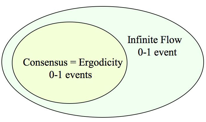
Figure 2: The ergodicity and consensus coincide a.s., and all three events assume 0-1 law for an i.i.d model.

Example 4.

Consider the independent identical random model where each $W(k)$ is equally likely to be any of the $m\times m$ permutation matrices. Then, in view of the uniform distribution, we have $\mathsf{E}\!\left[W(k)\right]=\frac{1}{m}\,ee^{T}$ for all $k$. Hence, by Theorem 3, it follows that the infinite flow event $\mathscr{F}$ is happening almost surely. But, since the chain $\{W(k)\}$ is a sequence of permutation matrices, the consensus event $\mathscr{C}$ never happens. $\square$

3.3 Random Model and Its Expected Model

Here, we investigate the properties of an independent random model and its corresponding expected model. We establish two results in forthcoming Theorems 3 and 4 that later on play an important role in the establishment the Infinite Flow Theorem in Section 5. The first result shows the equivalence of the infinite flow property for a random chain $\{W(k)\}$ and its expected chain $\{\mathsf{E}\!\left[W(k)\right]\}$, as given in the following theorem.

Theorem 3.

Let $\{W(k)\}$ be an independent random model. Then, the model has infinite flow property if and only if the expected model has infinite flow property.

Proof.

Let $S\subset[m]$ be nontrivial. Since the model is independent, the random variables $W_{S}(k)$ are independent. By the definition of $W_{S}(k)$ and the stochasticity of $W(k)$, we have $0\leq W_{S}(k)\leq\sum_{i=1}^{m}\sum_{j=1}^{m}W_{ij}(k)=m$ for all $k\geq 0$. Thus, by monotone convergence theorem ([34], page 225), the infinite flow property of the model implies the infinite flow property of the expected model. On the other hand, since the model is independent and $0\leq W_{S}(k)\leq m$, by Kolmogorov’s three-series theorem ([34], page 64) it follows that: if $\sum_{k=0}^{\infty}\mathsf{E}\!\left[W_{S}(k)\right]=\infty$, then $\mathsf{Pr}\left(\sum_{k=0}^{\infty}W_{S}(k)=\infty\right)>0$. Since $\sum_{k=0}^{\infty}W_{S}(k)$ is a trivial event, we have $\mathsf{Pr}\left(\sum_{k=0}^{\infty}W_{S}(k)=\infty\right)=1$. Thus, since $S\subset[m]$ is arbitrary, the model has infinite flow property.  Q.E.D.

There is no analog of Theorem 3 for the ergodicity or consensus event, unless additional assumptions are imposed. However, a weaker result holds as seen in the following.

Lemma 6.

Let $\{W(k)\}$ be an independent model and assume that the model admits consensus (is ergodic). Then, the expected model $\{\mathsf{E}\!\left[W(k)\right]\}$ reaches a consensus (is ergodic).

The proof of Lemma 6 can be found in [5, 6].

The following theorem states another important result for later use. As a consequence of Lemma 6, and Theorems 1 and 3, the result provides an equivalent deterministic characterization of the ergodicity for a class of independent models.

Theorem 4.

Let $\{W(k)\}$ be an independent random model such that $\mathscr{E}=\mathscr{F}$ almost surely. Then, the model is ergodic if and only if the expected model is ergodic.

Proof.

If the ergodicity event is almost sure, then by Lemma 6, the expected model is ergodic. For the converse statement, let the chain $\{\mathsf{E}\!\left[W(k)\right]\}$ be ergodic. Then, by Theorem 1 the chain $\{\mathsf{E}\!\left[W(k)\right]\}$ has infinite flow. Therefore, by Theorem 3 the infinite flow event $\mathscr{F}$ is almost sure, and since $\mathscr{E}=\mathscr{F}$ a.s., the ergodicity event is almost sure.  Q.E.D.

4 Model with Feedback Property and Steady State in Expectation

In this section, we discuss two properties of a random model that are important in the development of our main results in Section 5. In particular, we introduce and study a model with feedback properties and a model with a common steady state in expectation. Stronger forms of these properties have always been used when establishing consensus both for deterministic and random models. Here, we provide some new fundamental insights into these properties.

4.1 Feedback Properties

We define several types of feedback property. Recall that $W^{i}$ denotes the $i$th column vector of a matrix $W$.

Definition 2.

A random model $\{W(k)\}$ has strong feedback property if there exists $\gamma>0$ such that

$$W_{ii}(k)\geq\gamma\qquad\hbox{a.s. for all $k\geq 0$ and all $i\in[m]$}.$$

The model has feedback property if there exists $\gamma>0$ such that

$$\mathsf{E}\!\left[W_{ii}(k)W_{ij}(k)\right]\geq\gamma\,\mathsf{E}\!\left[W_{ij}(k)\right],$$

for all $k\geq 0$, and all $i,j\in[m]$ with $i\not=j$. The model has weak feedback property if there exists $\gamma>0$ such that

$$\mathsf{E}\!\left[\left(W^{i}(k)\right)^{T}W^{j}(k)\right]\geq\gamma\left(\mathsf{E}\!\left[W_{ij}(k)\right]+\mathsf{E}\!\left[W_{ji}(k)\right]\right)$$

for all $k\geq 0$, and all $i,j\in[m]$ with $i\not=j$. The scalar $\gamma$ is referred to as a feedback constant.

While the difference between feedback and strong feedback property is apparent, the difference between weak feedback and feedback property may not be so obvious. The following example illustrates the difference between these concepts.

Example 5.

Consider the static deterministic chain $\{A(k)\}$:

$$A(k)=A=\left[\begin{array}[]{ccc}0&\frac{1}{2}&\frac{1}{2}\\ \frac{1}{2}&0&\frac{1}{2}\\ \frac{1}{2}&\frac{1}{2}&0\end{array}\right]\qquad\mbox{for $k\geq 0$}.$$

Since $A_{ii}A_{ij}=0$ and $A_{ij}\neq 0$ for all $i\neq j$, the model does not have feedback property. At the same time, since $A_{ij}+A_{ji}=1$ for $i\neq j$, it follows $(A^{i})^{T}A^{j}=\frac{1}{4}=\frac{1}{4}(A_{ij}+A_{ji})$. Thus, $\{A(k)\}$ has weak feedback property with $\gamma=\frac{1}{4}$. $\square$

It can be seen that strong feedback property implies feedback property, which in turn implies weak feedback property. The deterministic consensus and averaging models in [19, 21, 26, 29] require that the matrices have non-zero diagonal entries and uniformly bounded non-zero entries, which is more restrictive than the strong feedback property.

We next show that the feedback property of a random model implies the strong feedback property of its expected model.

Lemma 7.

Let a random model $\{W(k)\}$ have feedback property with constant $\gamma$. Then, its expected model $\{\mathsf{E}\!\left[W(k)\right]\}$ has strong feedback property with $\frac{\gamma}{m}.$

Proof.

Let the model have feedback property with a constant $\gamma$. Then, by the definition of the feedback property, we have $\mathsf{E}\!\left[W_{ii}(k)W_{ij}(k)\right]\geq\gamma\,\mathsf{E}\!\left[W_{ij}(k)\right]$ for any $k\geq 0$ and $i,j\in[m]$ with $i\not=j$. Since $W_{ij}(k)\leq 1$, it follows that

$$\mathsf{E}\!\left[W_{ii}(k)\right]\geq\mathsf{E}\!\left[W_{ii}(k)W_{ij}(k)\right]\geq\gamma\,\mathsf{E}\!\left[W_{ij}(k)\right]$$

for all $i,j\in[m],i\neq j$. The matrices $W(k)$ are stochastic, so that we have $\sum_{j=1}^{m}\mathsf{E}\!\left[W_{ij}(k)\right]=1$. Hence, for every $k\geq 0$ and $i\in[m]$, there exists an index $j^{*}$ (the dependence on $k$ and $i$ is suppressed) such that $\mathsf{E}\!\left[W_{ij^{*}}(k)\right]\geq\frac{1}{m}$. If $j^{*}=i$, then we are done; otherwise we have $\mathsf{E}\!\left[W_{ii}(k)\right]\geq\gamma\ \mathsf{E}\!\left[W_{ij^{*}}(k)\right]\geq\frac{\gamma}{m}$ for all $i\in[m]$. Hence, the expected chain has the strong feedback property with constant $\frac{\gamma}{m}$.  Q.E.D.

We now focus on an independent model. We have the following result.

Lemma 8.

Consider an independent model $\{W(k)\}$. Suppose that the model is such that there is an $\eta>0$ with the following property: for all $k\geq 0$ and $i,j\in[m]$ with $i\neq j$,

$$\mathsf{E}\!\left[W_{ij}(k)\right]>0\quad\implies\quad\mathsf{E}\!\left[W_{ii}(k)W_{ij}(k)\right]\geq\eta,$$

or the following property:
for all $k\geq 0$ and $i,j\in[m]$ with $i\neq j$,

$$\mathsf{E}\!\left[W_{ij}(k)\right]>0\quad\implies\quad\mathsf{E}\!\left[\left(W^{i}(k)\right)^{T}W^{j}(k)\right]\geq\eta.$$

Then, respectively, the model has feedback property with constant $\eta$ or weak feedback property with constant $\eta/2$.

Proof.

We prove only the case of feedback property, since the other case uses the same line of argument. If $\mathsf{E}\!\left[W_{ij}(k)\right]=0$ for some $k$ and $i,j$ with $i\neq j$, then the relation $\mathsf{E}\!\left[W_{ii}(k)W_{ij}(k)\right]\geq\eta\,\mathsf{E}\!\left[W_{ij}(k)\right]$ is satisfied trivially (with both sides equal to zero). If $\mathsf{E}\!\left[W_{ij}(k)\right]>0$, then by the assumption of the lemma, we have $\mathsf{E}\!\left[W_{ij}(k)W_{ii}(k)\right]\geq\eta$. Furthermore, since $1\geq W_{ij}(k)$ for all $i,j$ and $k$, it follows that $\mathsf{E}\!\left[W_{ij}(k)W_{ii}(k)\right]\geq\eta\geq\eta\,\mathsf{E}\!\left[W_{ij}(k)\right],$ thus showing that the model has feedback property with constant $\eta$.  Q.E.D.

The i.i.d. models $\{W(k)\}$ with almost surely positive diagonal entries $W_{ii}(k)$ have been studied in [6, 5, 7]. Such models have feedback property as seen in the following corollary.

Corollary 1.

If $\{W(k)\}$ is an i.i.d. model with almost surely positive diagonal entries, then the model has feedback property with constant

$\gamma=\min_{\{i\neq j\mid\mathsf{E}\!\left[W_{ij}(k)\right]>0\}}\ \mathsf{E}\!\left[W_{ii}(k)W_{ij}(k)\right]$.

Proof.

Let $\mathsf{E}\!\left[W_{ij}(k)\right]>0$ for some $i,j\in[m]$. Since $W_{ii}(k)>0$ a.s. and $W_{ij}(k)\geq 0$, we have $\mathsf{E}\!\left[W_{ii}(k)W_{ij}(k)\right]>0$. Define $\eta=\min_{\{i\neq j\mid\mathsf{E}\!\left[W_{ij}(k)\right]>0\}}\ \mathsf{E}\!\left[W_{ii}(k)W_{ij}(k)\right]$. Since the model is i.i.d., the constant $\eta$ is independent of time. Hence, by Lemma 8 it follows that the model has feedback property with constant $\eta$.  Q.E.D.

4.2 Steady State in Expectation

Here, we consider a model with another special property. Specifically, we discuss a random model $\{W(k)\}$ such that its expected chain $\{\mathsf{E}\!\left[W(k)\right]\}$ has a common steady state.

Definition 3.

A random model has a common steady state in expectation if there is a stochastic vector $\pi\in\mathbb{R}^{m}$ such that $\pi^{T}E[W(k)]=\pi^{T}$ for all $k$.

For example, the $m\times m$ matrices that are doubly stochastic in expectation satisfy the preceding definition with $\pi=\frac{1}{m}\,e$, such as the matrices arising in a randomized broadcast or gossip over a connected (static) network [13, 11].

Consider the function given by

$$V(x)=\sum_{i=1}^{m}\pi_{i}\left(x_{i}-\pi^{T}x\right)^{2}\qquad\hbox{for $x\in\mathbb{R}^{m}$}.$$ (6)

The function $V(x)$ measures the weighted spread of the vector $x$ entries with respect to the weighted average value $\pi^{T}x$.

We at first study the behavior of the weighted averages $\pi^{T}x(k)$ along the sequence $\{x(k)\}$. The main observation is that the random scalar sequence $\{\pi^{T}x(k)\}$ is a bounded martingale, which leads us to the following result.

Lemma 9.

Let $\{W(k)\}$ be an independent random model with a common steady state $\pi$ in expectation. Then, the sequence $\{\pi^{T}x(k)\}$ converges almost surely for any $x(0)\in\mathbb{R}^{m}$.

Proof.

By the model independency and $\pi^{T}\mathsf{E}\!\left[W(k)\right]=\pi^{T}$, it follows that the process $\{\pi^{T}x(k)\}$ is a martingale with respect to the natural filtration of the process for any initial $x(0)\in\mathbb{R}^{m}$. Since the matrices $W(k)$ are stochastic, the sequence $\{x(k)\}$ is bounded. Thus, $\{\pi^{T}x(k)\}$ is a bounded martingale. By the martingale convergence theorem (see [35], Theorem 35.5), the sequence $\{\pi^{T}x(k)\}$ converges a.s.  Q.E.D.

We next characterize the limit of the martingale $\{\pi^{T}x(k)\}$. Let $\lambda_{i,\pi}\in\mathbb{R}$ be the limit of the martingale $\{\pi^{T}x(k)\}$ for the initial state $x(0)=e_{i}$, and let $\lambda_{\pi}$ be the vector defined by

$$\lambda_{\pi} =(\lambda_{1,\pi},\ldots,\lambda_{m,\pi})$$ (7)

$$\hbox{with }\lambda_{i,\pi}=\lim_{k\to\infty}\pi^{T}W(k)\cdots W(0)e_{i}\ \ \hbox{for $i\in[m]$}.$$

In the following lemma, we provide some properties of the random vector $\lambda_{\pi}$.

Lemma 10.

Let $\{W(k)\}$ be an independent model with a common steady state $\pi$ in expectation. Then, the random vector $\lambda_{\pi}$ has the following properties:

1. $\lim_{k\to\infty}\pi^{T}x(k)=\lambda^{T}_{\pi}x(0)$ a.s. for any $x(0)\in\mathbb{R}^{m}$.

2. $\lambda_{\pi}$ is a stochastic vector.

3. $\mathsf{E}\!\left[\lambda_{\pi}\right]=\pi$.

4. For every $x(0)\in\mathbb{R}^{m}$, the limit points of the sequence $\{x(k)\}$ lie in the random hyperplane $\mathcal{H}_{\pi,\lambda_{\pi}^{T}x(0)}=\{x\in\mathbb{R}^{m}\mid\pi^{T}x=\lambda_{\pi}^{T}x(0)\}$ almost surely.

Proof.

By Lemma 9 and the definition of $\lambda_{i\pi}$, we have $\lim_{k\to\infty}\pi^{T}x(k)=\lambda_{i\pi}$ almost surely for initial state $e_{i}$. Using the linearity of the system in (1), we obtain for any $x(0)\in\mathbb{R}^{m}$,

$$\lim_{k\to\infty}\pi^{T}x(k) =\sum_{i=1}^{m}x_{i}(0)\left(\lim_{k\to\infty}\pi^{T}W(k-1)\cdots W(0)e_{i}\right)$$

$$=\sum_{i=1}^{m}x_{i}(0)\lambda_{i,\pi}=\lambda^{T}_{\pi}x(0),$$ (8)

thus showing part (a).

Since $x(k)=W(k-1)\cdots W(0)x(0)$, by part (a) it follows $\lim_{k\to\infty}\pi^{T}W(k-1)\cdots W(0)=\lambda^{T}_{\pi}$. The matrices $W(k)$ and the vector $\pi$ have nonnegative entries implying that the vector $\lambda_{\pi}$ also has nonnegative entries. By letting $x(0)=e$ and using the stochasticity of $W(k)$, we have $x(k)=e$ for all $k$, implying $1=\pi^{T}x(k)$ for all $k$. Thus, we have $1=\lim_{k\to\infty}\pi^{T}x(k)=\lambda_{\pi}^{T}x(0)=\lambda_{\pi}^{T}e,$ where the second equality holds by part (a). Hence, $\lambda_{\pi}$ is a stochastic vector.

To show part (c), we note that by the martingale property of the process $\{\pi^{T}x(k)\}$, we have $\mathsf{E}\!\left[\pi^{T}x(k)\right]=\pi^{T}x(0)$ for all $k\geq 0$ and $x(0)\in\mathbb{R}^{m}$. By the boundedness of the martingale, we have $\lim_{k\to\infty}\mathsf{E}\!\left[\pi^{T}x(k)\right]=\mathsf{E}\!\left[\lambda_{\pi}^{T}\right]x(0)$ for any $x(0)\in\mathbb{R}^{m}$. The preceding two relations imply $\mathsf{E}\!\left[\lambda_{\pi}\right]=\pi$.

For part (d), we note that the sequence $\{x(k)\}$ is bounded for every $x(0)\in\mathbb{R}^{m}$ by the stochasticity of $W(k)$; thus, it has accumulation points. By part (a), each accumulation point $x^{*}$ of the sequence satisfies $\pi^{T}x^{*}=\lambda_{\pi}^{T}x(0)$ a.s.  Q.E.D.

We now focus on the sequence $\{V(x(k))\}$. We show that it is a convergent supermartingale, which indicates that $V(x)$ is a stochastic Lyapunov function for the random system in (1).

Theorem 5.

Let the random model $\{W(k)\}$ be independent with a common steady state $\pi$ in expectation. Then, we almost surely have for all $k\geq 0$,

$$\mathsf{E}\!\left[V(x(k+1))\mid x(k)\right]$$ (9)

$$\qquad\leq V(x(k))-\sum_{i<j}H_{ij}(k)\left(x_{i}(k)-x_{j}(k)\right)^{2},$$

where $H(k)=\mathsf{E}\!\left[W^{T}(k)DW(k)\right]$. Furthermore, $\{V(x(k))\}$ converges almost surely.

Proof.

By using $D=diag(\pi)$, from the definition of the function $V(x)$ in (6) we have

$$V(x)=x^{T}(I-\pi e^{T})D(I-e\pi^{T})x=x^{T}(D-\pi\pi^{T})x,$$

where the second equality is obtained by using $e^{T}D=\pi^{T}$, $De=\pi$, and $\pi^{T}e=1$. In view of $x(k+1)=W(k)x(k)$, it follows that for all $k\geq 0$,

$$V(x(k+1)) =x(k+1)^{T}(D-\pi\pi^{T})x(k+1)$$ (10)

$$=x(k)W(k)^{T}(D-\pi\pi^{T})W(k)x(k).$$ (11)

Since the model is independent, by taking the expectation conditioned on $x(k)$, we obtain

$$\mathsf{E}\!\left[V(x(k+1))\mid x(k)\right]=x(k)^{T}\mathsf{E}\!\left[W(k)^{T}(D-\pi\pi^{T})W(k)\right]x(k),$$

almost surely for all $k\geq 0$. Since $H(k)=\mathsf{E}\!\left[W^{T}(k)DW(k)\right]$, we further have

$$\mathsf{E}\!\left[V(x(k+1))\mid x(k)\right]$$

$$=x(k)^{T}H(k)x(k)-\mathsf{E}\!\left[\left(\pi^{T}W(k)x(k)\right)^{2}\mid x(k)\right]$$

$$\leq x(k)^{T}H(k)x(k)-\left(\mathsf{E}\!\left[\pi^{T}W(k)x(k)\mid x(k)\right]\right)^{2},$$

where the inequality follows by Jensen’s inequality (see [34], page 225) and the convexity of the function $s\mapsto s^{2}$. The expected matrices $\mathsf{E}\!\left[W(k)\right]$ have the same steady state $\pi$, implying that almost surely for all $k\geq 0$,

$$\mathsf{E}\!\left[\pi^{T}W(k)x(k)\mid x(k)\right]=\pi^{T}\mathsf{E}\!\left[W(k)\right]x(k)=\pi^{T}x(k).$$

By combining the preceding two relations, we see that almost surely for all $k\geq 0$,

$$\mathsf{E}\!\left[V(x(k+1))\mid x(k)\right]\leq x(k)^{T}\left(H(k)-\pi\pi^{T}\right)x(k).$$

By adding and subtracting $x(k)^{T}Dx(k)$ to the right hand side of the preceding relation and using (10), we obtain almost surely

$$\mathsf{E}\!\left[V(x(k+1))\mid x(k)\right]$$ (12)

$$\leq x(k)^{T}\left(H(k)-D\right)x(k)+V(x(k))\ \ \hbox{ for all $k\geq 0$}.$$

Now, we show that $x(k)^{T}\left(H(k)-D\right)x(k)=\sum_{i<j}H_{ij}(k)(x_{i}(k)-x_{j}(k))^{2}$. By the definition of $H(k)$ we have $H_{ij}(k)=\sum_{\ell=1}^{m}\mathsf{E}\!\left[\pi_{\ell}W_{\ell i}(k)W_{\ell j}(k)\right]$, so that for $i\in[m]$,

$$\sum_{j=1\atop j\not=i}^{m}H_{ij}(k) =\mathsf{E}\!\left[\sum_{j=1\atop j\not=i}^{m}\sum_{\ell=1}^{m}\pi_{\ell}W_{\ell i}(k)W_{\ell j}(k)\right]$$

$$=\mathsf{E}\!\left[\sum_{\ell=1}^{m}\pi_{\ell}W_{\ell i}(k)\sum_{j=1\atop j\not=i}^{m}W_{\ell j}(k)\right].$$

Since $W(k)$ is stochastic, we have $\sum_{j=1,j\not=i}^{m}W_{\ell j}(k)=1-W_{\ell i}(k)$, implying that

$$\sum_{j=1\atop j\not=i}^{m}H_{ij}(k) =\mathsf{E}\!\left[\sum_{\ell=1}^{m}\pi_{\ell}W_{\ell i}(k)\right]-\mathsf{E}\!\left[\sum_{\ell=1}^{m}\pi_{\ell}W^{2}_{\ell i}(k)\right]$$

$$=\pi_{i}-H_{ii}(k),$$

where the last equality follows from $\mathsf{E}\!\left[\pi^{T}W(k)\right]=\pi^{T}$. Since $D=diag(\pi)$, the preceding relation yields

$$H_{ii}(k)=D_{ii}-\sum_{j=1\atop j\not=i}^{m}H_{ij}(k).$$ (13)

Therefore, for any $x\in\mathbb{R}^{m}$, we have $x^{T}H(k)x=\sum_{i=1}^{m}x_{i}\sum_{j=1}^{m}H_{ij}(k)x_{j}$, which can be further written as

$$x^{T}H(k)x =\sum_{i=1}^{m}x_{i}\sum_{j=1\atop j\neq i}^{m}H_{ij}(k)x_{j}+\sum_{i=1}^{m}x_{i}H_{ii}(k)x_{i}$$

$$=\sum_{i=1}^{m}x_{i}\sum_{j=1\atop j\neq i}^{m}H_{ij}(k)(x_{j}-x_{i})+\sum_{i=1}^{m}x_{i}D_{ii}x_{i},$$

where the last equality follows from relation (13). The matrix $H(k)=\mathsf{E}\!\left[W(k)^{T}DW(k)\right]$ is symmetric, so that

$$\sum_{i=1}^{m}x_{i}\sum_{j=1\atop j\neq i}^{m}H_{ij}(k)(x_{j}-x_{i})=-\sum_{i<j}H_{ij}(k)(x_{i}-x_{j})^{2},$$

implying that $x^{T}H(k)x=-\sum_{i<j}H_{ij}(k)(x_{i}-x_{j})^{2}+x^{T}Dx.$ Therefore, we have

$$x(k)^{T}\left(H(k)-D\right)x(k)=-\sum_{i<j}H_{ij}(k)\left(x_{i}(k)-x_{j}(k)\right)^{2}.$$

By combining the preceding relation with (12), we conclude that relation (9) holds a.s. for all $k\geq 0$.

Since each $W(k)$ is a stochastic matrix and $\pi$ is stochastic vector, the matrix $H(k)$ has nonnegative entries for all $k$. Hence, from the preceding relation it follows that $\{V(x(k))\}$ is a supermartingale. The convergence of $\{V(x(k))\}$ follows straightforwardly from the nonnegative supermartingale convergence (see [34], (2.11) Corollary, page 236.)  Q.E.D.

We conclude this section with another result for the weighted distance function $V(x)$. This result plays crucial role in establishing our result in Section 5.2.

Lemma 11.

Let $\pi\in\mathbb{R}^{m}$ be a stochastic vector, and let $x\in\mathbb{R}^{m}$ be such that $x_{1}\leq\cdots\leq x_{m}$. Then, we have

$$\frac{1}{(m-1)^{2}}\,V(x)\leq\frac{1}{x_{m}-x_{1}}\,\sum_{i=1}^{m-1}(x_{i+1}-x_{i})^{3}.$$

Proof.

We establish two relations

$$\frac{1}{m-1}\,V(x) \leq\sum_{i=1}^{m-1}(x_{i+1}-x_{i})^{2},$$ (14)

$$\sum_{i=1}^{m-1}\frac{(x_{i+1}-x_{i})^{2}}{m-1} \leq\sum_{i=1}^{m-1}\frac{(x_{i+1}-x_{i})^{3}}{x_{m}-x_{1}}.$$ (15)

Observe that the desired result follows from (14)–(15).

We now show relation (14). We have $x_{i}\leq x_{m}$ for all $i$. Since $\pi$ is stochastic, we also have $x_{m}\geq\pi^{T}x\geq x_{1}$. Thus, $V(x)=\sum_{i=1}^{m}\pi_{i}(x_{i}-\pi^{T}x)^{2}\leq(x_{m}-x_{1})^{2}$. By writing $x_{m}-x_{1}=\sum_{i=1}^{m-1}(x_{i+1}-x_{i})$, we obtain

$$(x_{m}-x_{1})^{2} =(m-1)^{2}\left(\frac{1}{m-1}\sum_{i=1}^{m-1}(x_{i+1}-x_{i})\right)^{2}$$

$$\leq(m-1)\sum_{i=1}^{m-1}(x_{i+1}-x_{i})^{2},$$

where the last inequality holds by the convexity of the function $s\mapsto s^{2}$. Using $V(x)\leq(x_{m}-x_{1})^{2}$ and the preceding relation we obtain relation (14).

To prove relation (15), we write $(x_{m}-x_{1})\sum_{i=1}^{m-1}(x_{i+1}-x_{i})^{2}$ as $\sum_{j=1}^{m-1}(x_{j+1}-x_{j})\sum_{i=1}^{m-1}(x_{i+1}-x_{i})^{2}$ , which is equal to $\sum_{j=1}^{m-1}(x_{j+1}-x_{j})^{3}+\Delta$ with $\Delta$ given by

$$\sum_{j<i}\left((x_{j+1}-x_{j})(x_{i+1}-x_{i})^{2}+(x_{i+1}-x_{i})(x_{j+1}-x_{j})^{2}\right).$$

To estimate $\Delta$, we consider scalars $\alpha\geq 0$ and $\beta\geq 0$, and let $u=(\alpha,\beta)$ and $v=(\beta^{2},\alpha^{2})$. Then, by Hölder’s inequality with $p=3$, $q=\frac{3}{2}$, we have $u^{T}v\leq\|u\|_{p}\,\|v\|_{q}$, where $\|\cdot\|_{p}$ is the $p$-norm. Hence,

$$\alpha\beta^{2}+\beta\alpha^{2}\leq\left(\alpha^{3}+\beta^{3}\right)^{\frac{1}{3}}\left(\beta^{3}+\alpha^{3}\right)^{\frac{2}{3}}=\alpha^{3}+\beta^{3}.$$ (16)

By using (16) with $\alpha_{j}=(x_{j+1}-x_{j})$ and $\beta_{i}=(x_{i+1}-x_{i})$ for different indices $j$ and $i$, $1\leq j<i\leq m-1$, we obtain

$$(x_{m}-x_{1})\sum_{i=1}^{m-1}(x_{i+1}-x_{i})^{2}$$

$$\leq\sum_{j=1}^{m-1}(x_{j+1}-x_{j})^{3}+\sum_{j<i}\left((x_{j+1}-x_{j})^{3}+(x_{i+1}-x_{i})^{3}\right)$$

$$=(m-1)\,\sum_{i=1}^{m-1}(x_{i+1}-x_{i})^{3},$$

which completes the proof.  Q.E.D.

5 Model with Infinite Flow Property

We consider an independent random model with infinite flow. We show that this property, together with weak feedback and a common steady state in expectation, is necessary and sufficient for almost sure ergodicity. Moreover, we establish that the ergodicity of the model is equivalent to the ergodicity of the expected model.

5.1 Preliminary Result

We now provide an important relation that we use later on in Section 5.2.

Lemma 12.

Let $\{A(k)\}\subset\mathbb{S}^{m}$ and $z(k+1)=A(k)z(k)$ for all $k\geq 0$ and some $z(0)\in\mathbb{R}^{m}.$ Let $\sigma$ be a permutation of the index set $[m]$ corresponding to the nondecreasing ordering of the entries $z_{\ell}(0)$, i.e., $\sigma$ is a permutation on $[m]$ such that $z_{\sigma_{1}}(0)\leq\cdots\leq z_{\sigma_{m}}(0)$. Also, let $T\geq 1$ be such that

$$\sum_{k=0}^{T-1}A_{S}(k)\geq\delta\qquad\hbox{for every $S\subset[m]$},$$ (17)

where $\delta\in(0,1)$ is arbitrary. Then, we have

$$\sum_{k=0}^{T-1}\sum_{i<j}\left(A_{ij}(k)+A_{ji}(k)\right)(z_{j}(k)-z_{i}(k))^{2}$$

$$\geq\frac{\delta(1-\delta)^{2}}{z_{\sigma_{m}}(0)-z_{\sigma_{1}}(0)}\sum_{i=1}^{m-1}(z_{\sigma_{i+1}}(0)-z_{\sigma_{i}}(0))^{3}.$$

Proof.

Relation (17) holds for any nontrivial set $S\subset[m]$. Hence, without loss of generality we may assume that the permutation $\sigma$ is identity (otherwise we will relabel the indices of the entries in $z(0)$ and update the matrices accordingly). Thus, we have $z_{1}(0)\leq\cdots\leq z_{m}(0)$. For each $\ell=1,\ldots,m-1$, let $S_{\ell}=\{1,\ldots,\ell\}$ and define time $t_{\ell}\geq 1$, as follows:

$$t_{\ell}=\mathop{\rm argmin}_{t\geq 1}\left\{\sum_{k=0}^{t-1}\ A_{S_{\ell}}(k)\geq\delta\,\frac{z_{\ell+1}(0)-z_{\ell}(0)}{z_{m}(0)-z_{1}(0)}\right\}.$$

Since the entries of $z(0)$ are nondecreasing, we have $\delta\frac{z_{\ell+1}(0)-z_{\ell}(0)}{(z_{m}(0)-z_{1}(0))}\leq\delta$ for all $\ell=1,\ldots,m-1$. Thus, by relation (17), the time $t_{\ell}\geq 1$ exists and $t_{\ell}\leq T$ for each $\ell$.

We next estimate $z_{j}(k)-z_{i}(k)$ for all $i<j$ and any time $k=0,\cdots,T-1$. For this, we introduce for $0\leq k\leq T-1$ and $i<j$ the index sets $a_{ij}(k)\subset[m]$, as follows:

$$a_{ij}(k)=\{\ell\in[m]\mid k\leq t_{\ell}-1,\ \ell\geq i,\ \ell+1\leq j\}.$$

Let $k\leq t_{\ell}-1$ for some $\ell$. Since $S_{\ell}=\{1,\ldots,\ell\}$, we have $i\in S_{\ell}$ and $j\in\bar{S}_{\ell}$. Thus, by Lemma 1 we have for any $k\geq 1$,

$$z_{i}(k)\leq\max_{s\in S_{\ell}}z_{s}(0)+(z_{m}(0)-z_{1}(0))\sum_{\tau=0}^{k-1}A_{S_{\ell}}(\tau),$$

$$z_{j}(k)\geq\min_{r\in\bar{S}_{\ell}}z_{r}(0)-(z_{m}(0)-z_{1}(0))\sum_{\tau=0}^{k-1}A_{S_{\ell}}(\tau).$$

Furthermore, $\max_{s\in S_{\ell}}z_{s}(0)=z_{\ell}(0)$ and $\min_{r\in\bar{S}_{\ell}}z_{r}(0)=z_{l+1}(0)$ since $S_{\ell}=\{1,\ldots,\ell\}$ and $z_{1}(0)\leq\cdots\leq z_{m}(0)$. Thus, it follows

$$z_{i}(k)-z_{\ell}(0)\leq(z_{m}(0)-z_{1}(0))\sum_{\tau=0}^{k-1}A_{S_{\ell}}(\tau),$$

$$z_{\ell+1}(0)-z_{j}(k)\leq(z_{m}(0)-z_{1}(0))\sum_{\tau=0}^{k-1}A_{S_{\ell}}(\tau).$$

By the definition of time $t_{\ell}$, we have $(z_{m}(0)-z_{1}(0))\sum_{\tau=0}^{k-1}A_{S_{\ell}}(\tau)<\delta\left(z_{\ell+1}(0)-z_{\ell}(0)\right)$ for $k\leq t_{\ell}-1$. Hence, by using this and the definition of $a_{ij}(k)$, for any $\ell\in a_{ij}(k)$ we have

$$z_{i}(k)-z_{\ell}(0) \leq\delta(z_{\ell+1}(0)-z_{\ell}(0)),$$ (18)

$$z_{\ell+1}(0)-z_{j}(k) \leq\delta(z_{\ell+1}(0)-z_{\ell}(0)).$$ (19)

Now suppose that $a_{ij}(k)=\{\ell_{1},\ldots,\ell_{r}\}$ for some $r\leq m-1$ and $\ell_{1}\leq\cdots\leq\ell_{r}$. By choosing $\ell=\ell_{1}$ in (18) and $\ell=\ell_{r}$ in (19), and by letting $\alpha_{i}=z_{i+1}(0)-z_{i}(0)$, we obtain

$$z_{j}(k)-z_{i}(k)\geq z_{\ell_{r}+1}(0)-z_{\ell_{1}}(0)-\delta(\alpha_{\ell_{r}}+\alpha_{\ell_{1}}).$$

Since $z_{i}(0)\leq z_{i+1}(0)$ for all $i=1,\ldots,m-1$, we have $z_{\ell_{1}}(0)\leq z_{\ell_{1}+1}(0)\leq\cdots\leq z_{\ell_{r}}(0)\leq z_{\ell_{r}+1}(0)$, which combined with the preceding relation yields $z_{j}(k)-z_{i}(k)\geq\sum_{\xi=1}^{r}(z_{\ell_{\xi}+1}(0)-z_{\ell_{\xi}}(0))-\delta(\alpha_{\ell_{r}}+\alpha_{\ell_{1}})$. Using $\alpha_{i}=z_{i+1}(0)-z_{i}(0)$ and $a_{ij}(k)=\{\ell_{1},\ldots,\ell_{r}\}$, we further have

$$z_{j}(k)-z_{i}(k) \geq\sum_{\xi=1}^{r}\alpha_{\ell_{\xi}}-\delta(\alpha_{\ell_{r}}+\alpha_{\ell_{1}})$$ (20)

$$\geq(1-\delta)\sum_{\xi=1}^{r-1}\alpha_{\ell_{\xi}}=(1-\delta)\sum_{\ell\in a_{ij}(k)}\alpha_{\ell}.$$

By Eq. 20, it follows that

$$\sum_{i<j}\left(A_{ij}(k)+A_{ji}(k)\right)(z_{j}(k)-z_{i}(k))^{2}$$

$$\quad\geq(1-\delta)^{2}\sum_{i<j}\left(A_{ij}(k)+A_{ji}(k)\right)\left(\sum_{\ell\in a_{ij}(k)}\alpha_{\ell}\right)^{2}$$

$$\quad\geq(1-\delta)^{2}\sum_{i<j}\left(A_{ij}(k)+A_{ji}(k)\right)\left(\sum_{\ell\in a_{ij}(k)}\alpha_{\ell}^{2}\right),$$

where the last inequality holds by $\alpha_{\ell}\geq 0$. In the last term in the preceding relation, the coefficient of $\alpha^{2}_{\ell}$ is equal to $(1-\delta)^{2}A_{S_{\ell}}(k)$. Furthermore, by the definition of $a_{ij}(k)$, we have $\ell\in a_{ij}(k)$ only when $k\leq t_{\ell}-1$. Therefore,

$$\sum_{i<j}\left(A_{ij}(k)+A_{ji}(k)\right)(z_{j}(k)-z_{i}(k))^{2}$$

$$\quad\geq(1-\delta)^{2}\sum_{i<j}\left(A_{ij}(k)+A_{ji}(k)\right)\left(\sum_{\ell\in a_{ij}(k)}\alpha^{2}_{\ell}\right)$$

$$\quad=(1-\delta)^{2}\sum_{\{\ell\mid k\leq t_{\ell}-1\}}A_{S_{\ell}}(k)\alpha^{2}_{\ell}.$$

Summing these relations over $k=0,\ldots,T-1$, we obtain

$$\sum_{k=0}^{T-1}\sum_{i<j}\left(A_{ij}(k)+A_{ji}(k)\right)(z_{j}(k)-z_{i}(k))^{2}$$

$$\quad\geq(1-\delta)^{2}\sum_{k=0}^{T-1}\sum_{\{\ell\mid k\leq t_{\ell}-1\}}A_{S_{\ell}}(k)\alpha^{2}_{\ell}$$

$$\quad\geq(1-\delta)^{2}\sum_{\ell=1}^{m-1}\left(\sum_{k=0}^{t_{\ell}-1}A_{S_{\ell}}(k)\right)\alpha_{\ell}^{2},$$

where the last inequality follows by exchanging the order of summation. By the definition of $t_{\ell}$ and using $\alpha_{\ell}=z_{\ell+1}(0)-z_{\ell}(0)$, we have $\sum_{k=0}^{t_{\ell}-1}A_{S_{\ell}}(k)\geq\frac{\delta\alpha_{\ell}}{z_{m}(0)-z_{1}(0)}$, implying

$$\sum_{k=0}^{T-1}\sum_{i<j}\left(A_{ij}(k)+A_{ji}(k)\right)(z_{j}(k)-z_{i}(k))^{2}$$

$$\qquad=\delta(1-\delta)^{2}\,\sum_{\ell=1}^{m-1}\frac{\alpha_{\ell}^{3}}{z_{m}(0)-z_{1}(0)}.$$

Q.E.D.

5.2 Sufficient Conditions for Ergodicity

We now establish one of our main results for independent random models with infinite flow property and having a common vector in expectation and weak feedback property.

Let $t_{0}=0$ and for any $q\geq 1$, let

$$t_{q}=\mathop{\rm argmin}_{t\geq t_{q-1}+1}\mathsf{Pr}\left(\min_{S\subset[m]}\ \sum_{k=t_{q-1}}^{t-1}W_{S}(k)\geq\delta\right)\geq\epsilon,$$ (21)

where $\epsilon,\delta\in(0,1)$ are arbitrary. Define

$$\mathscr{A}_{q}=\left\{\omega\,\Big{|}\,\min_{S\subset[m]}\sum_{k=t_{q}}^{t_{q+1}-1}W_{S}(k)(\omega)\geq\delta\right\}\quad\hbox{for $q\geq 0$}.$$ (22)

Since the model has infinite flow property, the infinite flow event $\mathscr{F}$ occurs a.s. Therefore, the time $t_{q}$ is finite for all $q$.

We next show that either the infinite flow or expected infinite flow property is sufficient for the ergodicity of the model.

Theorem 6.

(Sufficient Ergodicity Condition)  Let $\{W(k)\}$ be an independent random model with a common steady state $\pi>0$ in expectation and weak feedback property. Also, let the model have either infinite flow or expected infinite flow property. Then, the model is ergodic. In particular, $\lim_{k\to\infty}x_{i}(k)=\lambda_{\pi}^{T}x(0)$ almost surely for all $i\in[m],$ where $\lambda_{\pi}$ is the random vector of Eq. (7).

Proof.

Assume that the model has infinite flow property. Let $x(0)\in\mathbb{R}^{m}$ be arbitrary initial state. Let us denote the (random) ordering of the entries of the vector $x(t_{q})$ by $\eta^{q}$ for all $q$. Thus, at time $t_{q}$, we have $x_{\eta^{q}_{1}}(t_{q})\leq\cdots\leq x_{\eta^{q}_{m}}(t_{q})$.

Now, let $q\geq 0$ be arbitrary and fixed, and consider the set $\mathscr{A}_{q}$ in (22). By the definition of $\mathscr{A}_{q}$, we have $\sum_{k=t_{q}}^{t_{q+1}-1}W_{S}(k)(\omega)\geq\delta$ for any $S\subset[m]$ and $\omega\in\mathscr{A}_{q}$. Thus, by Lemma 12, we obtain for any $\omega\in\mathscr{A}_{q}$,

$$\sum_{t=t_{q}}^{t_{q+1}-1}\sum_{i<j}\ \left(W_{ij}(t)+W_{ji}(t)\right)(x_{i}(t)-x_{j}(t))^{2}(\omega)$$

$$\geq\frac{\delta(1-\delta)^{2}}{d(t_{q})(\omega)}\sum_{\ell=1}^{m-1}(x_{\eta^{q}_{\ell+1}}(t_{q})-x_{\eta^{q}_{\ell}}(t_{q}))^{3}(\omega)$$

$$\geq\frac{\delta(1-\delta)^{2}}{(m-1)^{2}}\,V(x(t_{q}))(\omega),$$

where $d(t_{q})=x_{\eta^{q}_{m}}(t_{q})-x_{\eta^{q}_{1}}(t_{q})$ and the last inequality follows by Lemma 11. We can compactly write the inequality as:

$$\sum_{t=t_{q}}^{t_{q+1}-1}\ \sum_{i<j}\left(W_{ij}(t)+W_{ji}(t)\right)(x_{i}(t)-x_{j}(t))^{2}$$

$$\qquad\geq\frac{\delta(1-\delta)^{2}}{(m-1)^{2}}\ V(x(t_{q})){\it 1}_{\mathscr{A}_{q}},$$ (23)

where ${\it 1}_{\mathscr{A}_{q}}$ is the indicator function of the event ${\mathscr{A}_{q}}$.

Observe that $x(t)$ and $W(t)$ are independent since the model is independent. Therefore, by Theorem 5, we have

$$\mathsf{E}\!\left[V(x(t_{q+1}))-V(x(t_{q}))\right]$$

$$\leq-\sum_{t=t_{q}}^{t_{q}-1}\sum_{i<j}H_{ij}(t)\mathsf{E}\!\left[(x_{i}(t)-x_{j}(t))^{2}\right],$$

with $H(k)=\mathsf{E}\!\left[W^{T}(k)DW(k)\right]$ and $D=diag(\pi).$ Let $\pi_{\min}=\min_{\ell\in[m]}\pi_{\ell}$ and note that $\pi_{\min}>0$ by $\pi>0$. Thus,

$$H_{ij}(t) =\mathsf{E}\!\left[(W^{i}(t))^{T}DW^{j}(t)\right]$$

$$\geq\pi_{\min}\,\mathsf{E}\!\left[(W^{i}(t))^{T}W^{j}(t)\right]$$

$$\geq\pi_{\min}\,\gamma\,\left(\mathsf{E}\!\left[W_{ij}(t)\right]+\mathsf{E}\!\left[W_{ji}(t)\right]\right).$$

Therefore,

$$\mathsf{E}\!\left[V(x(t_{q+1}))\right]-\mathsf{E}\!\left[V(x(t_{q}))\right]$$

$$\leq-\pi_{\min}\,\gamma\,\mathsf{E}\!\left[\sum_{t=t_{q}}^{t_{q}-1}\sum_{i<j}\left(W_{ij}(t)+W_{ji}(t)\right)(x_{i}(t)-x_{j}(t))^{2}\right].$$

Further, by using relation (5.2), we obtain

$$\mathsf{E}\!\left[V(x(t_{q+1}))\right]-\mathsf{E}\!\left[V(x(t_{q}))\right]$$

$$\qquad\leq-\pi_{\min}\,\gamma\ \mathsf{E}\!\left[\frac{\delta(1-\delta)^{2}}{(m-1)^{2}}\,{\it 1}_{A_{q}}V(x(t_{q}))\right]$$

$$\qquad\leq-\frac{\epsilon\delta(1-\delta)^{2}\gamma\pi_{\min}}{(m-1)^{2}}\,\mathsf{E}\!\left[V(x(t_{q}))\right],$$

where the last inequality follows by $\mathsf{Pr}(\mathscr{A}_{q})\geq\epsilon$, and the fact that ${\it 1}_{\mathscr{A}_{q}}$ and $V(x(t_{q}))$ are independent (since $x(t_{q})$ depends on information prior to time $t_{q}$ and the set $\mathscr{A}_{q}$ relies on information at time $t_{q}$ and later). Hence, it follows

$$\mathsf{E}\!\left[V(x(t_{q+1}))\right]\leq\left(1-\frac{\epsilon\delta(1-\delta)^{2}\gamma\pi_{\min}}{(m-1)^{2}}\right)\mathsf{E}\!\left[V(x(t_{q}))\right].$$

Therefore, for arbitrary $q\geq 0$ we have

$$\mathsf{E}\!\left[V(x(t_{q}))\right]\leq\left(1-\frac{\epsilon\delta(1-\delta)^{2}\gamma\pi_{\min}}{(m-1)^{2}}\right)^{q}\mathsf{E}\!\left[V(x(0))\right],$$

implying that $\sum_{q=0}^{\infty}\mathsf{E}\!\left[V(x(t_{q}))\right]<\infty$. In view of the nonnegativity of $V(x)$, by the monotone convergence theorem ([35], Theorem 16.6) it follows $\mathsf{E}\!\left[\sum_{q=0}^{\infty}V(x(t_{q}))\right]<\infty$, implying $\lim_{q\rightarrow\infty}V(x(t_{q}))=0$ a.s. According to Theorem 5, the sequence $\{V(x(k))\}$ is convergent, which together with the preceding relation implies that $\lim_{k\rightarrow\infty}V(x(k))=0$ a.s.

To show the ergodicity of the model, we note that by the convergence result for the martingale $\{\pi^{T}x(k)\}$ in Lemma 10(a), we have $\lim_{k\to\infty}\pi^{T}x(k)=\lambda_{\pi}^{T}x(0)$ a.s., where the random vector $\lambda_{\pi}$ is given by Eq. (7). Now, using $\pi^{T}x(k)\to\lambda_{\pi}^{T}x(0)$ and the fact that all norms in $\mathbb{R}^{m}$ are equivalent, we obtain $\lim_{k\to\infty}|x_{i}(k)-\lambda_{\pi}^{T}x(0)|=0$ a.s. for all $i\in[m],$ thus showing the ergodicity of the model.

Assume now that $\{W(k)\}$ has expected infinite flow, i.e., $\sum_{k=0}^{\infty}\,\mathsf{E}\!\left[W_{S}(k)\right]=\infty$ for any nontrivial $S\subset[m]$. By Theorem 3, $\{W(k)\}$ has infinite flow property if and only if it has expected infinite flow, and the result follows by the preceding case.  Q.E.D.

5.3 Necessary and Sufficient Conditions for Ergodicity

Here, we provide the central result of this paper. The result establishes necessary and sufficient conditions for ergodicity of random models with weak feedback property and a common steady state $\pi>0$ in expectation. The conditions are reliant on infinite flow, and guarantee that the ergodicity of the model is equivalent to the ergodicity of the expected model. The result emerges as an outcome of several important results that we have developed so far. In particular, we combine the result $\mathscr{E}\subseteq\mathscr{F}$ stating that the ergodicity event is always contained in the infinite flow event (Theorem 1), the deterministic characterization of the infinite flow of Theorem 3, and the sufficient conditions of Theorem 6. We also make use of Theorem 4 providing conditions for equivalence of the ergodicity of the chain and the expected chain.

Theorem 7.

(Infinite Flow Theorem)  Let the random model $\{W(k)\}$ be independent, and have a common steady state $\pi>0$ in expectation and weak feedback property. Then, the following conditions are equivalent:

1. The model is ergodic.

2. The model has infinite flow property.

3. The expected model has infinite flow property.

4. The expected model is ergodic.

Proof.

First, we establish that parts (a), (b) and (c) are equivalent by showing that (a) $\implies$ (b) $\iff$ (c) $\implies$ (a). In particular, by Theorem 1 we have $\mathscr{E}\subseteq\mathscr{F}$, showing that (a) $\implies$ (b). By Theorem 3, parts (b) and (c) are equivalent. By Theorem 6, part (c) implies part (a). Now, we prove (a) $\iff$ (d). Since (a) $\iff$ (b), we have $\mathscr{E}=\mathscr{F}$ a.s. Hence, by Theorem 4, the parts (a) and (d) are equivalent.  Q.E.D.

The infinite flow theorem combined with the deterministic characterization of the infinite flow model of Theorem 3 leads us to the following result.

Corollary 2.

Let $\{A(k)\}\subset\mathbb{S}^{m}$ be a deterministic model that has a common steady state vector $\pi>0$ and weak feedback property. Then, the chain $\{A(k)\}$ is ergodic if and only if $\sum_{k=0}^{\infty}A_{S}(k)=\infty$ for every nontrivial $S\subset[m]$.

Under the conditions of Theorem 7, the model admits consensus, which follows directly from relation $\mathscr{E}\subseteq\mathscr{C}$.

Corollary 3.

Let the assumptions of Theorem 7 hold. Then, the model admits consensus.

The infinite flow theorem establishes the equivalence between the ergodicity of a chain and the expected chain for a class of independent random models. The central role in this result is played by the infinite flow and its equivalent deterministic characterization. Another crucial result is the interplay between the ergodicity and infinite flow of Theorem 4 yielding the equivalence between ergodicity of the chain and the expected chain. The following two examples are provided to illustrate some straightforward applications of the infinite flow theorem.

i.i.d. Models. Consider an i.i.d. model $\{W(k)\}$. Then, the expected matrix $\bar{W}=\mathsf{E}\!\left[W(k)\right]$ is independent of $k$. Since $\bar{W}$ is stochastic, we have $\pi^{T}\bar{W}=\pi^{T}$ for a stochastic vector $\pi\geq 0$. Therefore, an i.i.d. model is an independent model with a common steady state $\pi$ in expectation.

In [5], it is shown that for the class of i.i.d. models that have a.s. positive diagonal entries, the ergodicity of the expected model and the ergodicity of the original model are equivalent. The application of this result is reliant on the condition of the a.s. positive diagonal entries, which implies that the model has feedback property, as shown in Corollary 1. This property, however, is stronger than weak feedback property. At the same time, no requirement on the steady state vector is needed.

The application of the infinite flow theorem to the i.i.d. case would require weak feedback property and the existence of a steady state vector $\pi>0$. Thus, there is a tradeoff in the conditions for the ergodicity provided by the infinite flow theorem and those given in [5]. To further illustrate the difference in the conditions, we consider the homogeneous deterministic model $\{A(k)\}$ of Example 5. The model $\{A(k)\}$ has weak feedback property and the steady state vector $\pi=\frac{1}{3}e$, so the ergodicity of the model can be deduced from the infinite flow theorem. At the same time, as seen in Example 5, the model does not have positive diagonal entries and, therefore, the ergodicity of the model cannot be deduced from the results in [5, 7]. In the light of this, the infinite flow theorem provides conditions for ergodicity that complement the conditions of [5, 7].

Gossip Algorithms on Time-varying Networks. As another application of the infinite flow theorem, we consider an extension of the standard gossip algorithm to time-varying networks. In particular, the gossip algorithm originally proposed in [36, 11] is for static networks. Here, we give a sufficient condition for the convergence of a gossip algorithm for networks with time-changing topology. Consider a network of $m$ agents viewed as nodes of a graph with the node set $[m]$. Suppose that each agent has a private scalar value $x_{i}(0)$ at time $k=0$. Now, let the interactions of the agents be random at nonnegative integer valued time instances $k$ as follows: At any time $k\geq 1$, two different agents $i,j\in[m]$ wake up with probability $P_{ij}(k)$, where $P_{ij}(k)=P_{ji}(k)$ and $\sum_{i<j}P_{ij}(k)=1$. Then, they set their values to the average of their current values, i.e., $x_{i}(k)=x_{j}(k)=\frac{1}{2}(x_{i}(k-1)+x_{j}(k-1))$. The choices of the pairs $\{i,j\}$ of interacting agents at different time instances are independent.

Based on the agent interaction model, define the independent random model $\{W(k)\}$ by:

$$W(k)=I-\frac{1}{2}(e_{i}-e_{j})(e_{i}-e_{j})^{T}\ \mbox{with prob.\ $P_{ij}(k)$}.$$ (24)

Then, the dynamic system (1) driven by the random chain $\{W(k)\}$ describes the evolution of the vector $x(k)$ that has its $i$-th component value equal to agent $i$ value, $x_{i}(k)$. As seen from (24), any realization of the model $\{W(k)\}$ is doubly stochastic. Hence, the model has a common steady state $\pi=\frac{1}{m}e$ in expectation. Also, the model has strong feedback property (with $\gamma=\frac{1}{2}$).

Lemma 13.

For extended gossip algorithm (24), the consensus is almost sure if $\sum_{k=0}^{\infty}P_{S}(k)=\infty$ for any nontrivial set $S\subset[m]$.

Proof.

The extended gossip algorithm satisfies the assumption of the infinite flow Theorem 7. Since $\mathsf{E}\!\left[W_{ij}(k)+W_{ji}(k)\right]=P_{ij}(k)$ for all $i\neq j$ and $k\geq 0$, it follows that $\sum_{k=0}^{\infty}P_{S}(k)=\sum_{k=0}^{\infty}\mathsf{E}\!\left[W_{S}(k)\right]$. Thus, by the infinite flow theorem the model admits consensus if $\sum_{k=0}^{\infty}P_{S}(k)=\infty$ for any $S\subset[m]$.  Q.E.D.

When $P(k)=P$ for all $k$ as in [36, 11], we can consider the graph $G=([m],E)$ where the edge $\{i,j\}\in E$ if and only if $P_{ij}=P_{ji}>0$. In this case, it can be seen that the condition of Lemma 13 is equivalent to the requirement that the graph $G$ is connected. One can further modify the algorithm in (24) to allow for time-varying weights, i.e., $x_{i}(k)=a(k)x_{i}(k-1)+(1-a(k))x_{j}(k-1)$ and $x_{j}(k)=a(k)x_{j}(k-1)+(1-a(k))x_{i}(k-1)$ with $a(k)\in(0,1)$. Such a scheme is a natural generalization of the symmetric gossip model proposed in [6]. In this case, it can be verified that if $a(k)\in[a,1-a]$ for $a\in(0,\frac{1}{2}]$, then the result of Lemma 13 still holds.

6 Conclusion

We have studied the ergodicity and consensus problem for a linear discrete-time dynamic model driven by random stochastic matrices. We have introduced a concept of the infinite flow event and studied the relations among this event, ergodicity event and consensus event. The central result is the infinite flow theorem providing necessary and sufficient conditions for ergodicity of independent random models. The theorem captures the conditions ensuring the convergence of the random consensus algorithms, such as gossip and broadcast schemes [13, 12, 11]. Moreover, the infinite flow theorem captures simultaneously the conditions on the connectivity of the system and the sufficient information flow over time that have been important in studying the consensus and average consensus in deterministic settings [19, 20, 24, 26, 29, 37, 38]. As illustrated briefly on two examples, the infinite flow theorem provides a convenient tool for studying the ergodicity of a model as well as consensus algorithms. Finally, we note that the work in this paper is readily extendible to the case when the initial state $x(0)$ in (1) is itself random and independent of the chain $\{W(k)\}$.

References

- [1] M. Rosenblatt, “Products of independent identically distributed stochastic matrices,” Journal of Journal of Mathematical Analysis and Applications, vol. 11, no. 1, pp. 1–10, 1965.
- [2] K. Nawrotzki, “Discrete open systems on markov chains in a random environment. I,” Elektronische Informationsverarbeitung und Kybernetik, vol. 17, pp. 569–599, 1981.
- [3] ——, “Discrete open systems on markov chains in a random environment. II,” Elektronische Informationsverarbeitung und Kybernetik, vol. 18, pp. 83–98, 1982.
- [4] R. Cogburn, “On products of random stochastic matrices,” In Random matrices and their applications, pp. 199–213, 1986.
- [5] A. Tahbaz-Salehi and A. Jadbabaie, “A necessary and sufficient condition for consensus over random networks,” IEEE Transactions on Automatic Control, vol. 53, no. 3, pp. 791–795, 2008.
- [6] F. Fagnani and S. Zampieri, “Randomized consensus algorithms over large scale networks,” IEEE Journal on Selected Areas in Communications, vol. 26, no. 4, pp. 634–649, 2008.
- [7] A. Tahbaz-Salehi and A. Jadbabaie, “Consensus over ergodic stationary graph processes,” IEEE Transactions on Automatic Control, vol. 55, no. 1, pp. 225–230, 2010.
- [8] Y. Hatano, A. Das, and M. Mesbahi, “Agreement in presence of noise: Pseudogradients on random geometric networks,” in Proceedings of the 44th IEEE Conference on Decision and Control, and European Control Conference, 2005, pp. 6382–6387.
- [9] I. Lobel and A. Ozdaglar, “Distributed subgradient methods over random networks,” Laboratory for Information and Decision Systems, Report 2800, MIT, Tech. Rep., 2008.
- [10] S. Patterson, B. Bamieh, and A. E. Abbadi, “Distributed average consensus with stochastic communication failures,” IEEE Transactions on Signal processing, vol. 57, pp. 2748–2761, 2009.
- [11] S. Boyd, A. Ghosh, B. Prabhakar, and D. Shah, “Randomized gossip algorithms,” IEEE Transactions on Information Theory, vol. 52, no. 6, pp. 2508–2530, 2006.
- [12] A. Dimakis, A. Sarwate, and M. Wainwright, “Geographic gossip: Efficient averaging for sensor networks,” IEEE Transactions on Signal Processing, vol. 56, no. 3, pp. 1205–1216, 2008.
- [13] T. Aysal, M. Yildriz, A. Sarwate, and A. Scaglione, “Broadcast gossip algorithms for consensus,” IEEE Transactions on Signal processing, vol. 57, pp. 2748–2761, 2009.
- [14] P. F. R. Carli, F. Fagnani and S. Zampieri, “Gossip consensus algorithms via quantized communication,” Automatica, vol. 46, no. 1, pp. 70–80, 2010.
- [15] M. Huang and J. Manton, “Stochastic approximation for consensus seeking: Mean square and almost sure convergence,” in Proceedings of the 46th IEEE Conference on Decision and Control, 2007, pp. 306–311.
- [16] ——, “Coordination and consensus of networked agents with noisy measurements: Stochastic algorithms and asymptotic behavior,” SIAM Journal on Control and Optimization, vol. 48, no. 1, pp. 134–161, 2009.
- [17] S. Kar and J. Moura, “Distributed consensus algorithms in sensor networks: Link failures and channel noise,” IEEE Transactions on Signal Processing, vol. 57, no. 1, pp. 355–369, 2009.
- [18] B. Touri and A. Nedić, “Distributed consensus over network with noisy links,” in Proceedings of the 12th International Conference on Information Fusion, 2009, pp. 146–154.
- [19] J. Tsitsiklis, “Problems in decentralized decision making and computation,” Ph.D. dissertation, Dept. of Electrical Engineering and Computer Science, MIT, 1984.
- [20] J. Tsitsiklis and M. Athans, “Convergence and asymptotic agreement in distributed decision problems,” IEEE Transactions on Automatic Control, vol. 29, no. 1, pp. 42–50, 1984.
- [21] J. Tsitsiklis, D. Bertsekas, and M. Athans, “Distributed asynchronous deterministic and stochastic gradient optimization algorithms,” IEEE Transactions on Automatic Control, vol. 31, no. 9, pp. 803–812, 1986.
- [22] D. Bertsekas and J. Tsitsiklis, Parallel and Distributed Computation: Numerical Methods. Prentice-Hall Inc., 1989.
- [23] S. Li and T. Basar, “Asymptotic agreement and convergence of asynchronous stochastic algorithms,” IEEE Transactions on Automatic Control, vol. 32, no. 7, pp. 612–618, 1987.
- [24] A. Jadbabaie, J. Lin, and S. Morse, “Coordination of groups of mobile autonomous agents using nearest neighbor rules,” IEEE Transactions on Automatic Control, vol. 48, no. 6, pp. 988–1001, 2003.
- [25] R. Olfati-Saber and R. Murray, “Consensus problems in networks of agents with switching topology and time-delays,” IEEE Transactions on Automatic Control, vol. 49, no. 9, pp. 1520–1533, 2004.
- [26] A. Olshevsky and J. Tsitsiklis, “Convergence speed in distributed consensus and averaging,” SIAM Journal on Control and Optimization, vol. 48, no. 1, pp. 33–55, 2008.
- [27] W. Ren and R. Beard, “Consensus seeking in multi-agent systems under dynamically changing interaction topologies,” IEEE Transactions on Automatic Control, vol. 50, no. 5, pp. 655–661, 2005.
- [28] A. Kashyap, T. Basar, and R. Srikant, “Quantized consensus,” Automatica, vol. 43, no. 7, pp. 1192–1203, 2007.
- [29] A. Nedić, A. Olshevsky, A. Ozdaglar, and J. Tsitsiklis, “On distributed averaging algorithms and quantization effects,” 2009, to appear in IEEE Transactions on Automatic Control.
- [30] R. Carli, F. Fagnani, A. Speranzon, and S. Zampieri, “Communication constraints in the average consensus problem,” Automatica, vol. 44, no. 3, pp. 671–684, 2008.
- [31] R. Carli, F. Fagnani, P. Frasca, T. Taylor, and S. Zampieri, “Average consensus on networks with transmission noise or quantization,” in Proceedings of IEEE American Control Conference, 2007, pp. 4189–4194.
- [32] P. Bliman, A. Nedić, and A. Ozdaglar, “Rate of convergence for consensus with delays,” in Proceedings of the 47th IEEE Conference on Decision and Control, 2008.
- [33] S. Chatterjee and E. Seneta, “Towards consensus: Some convergence theorems on repeated averaging,” Journal of Applied Probability, vol. 14, no. 1, pp. 89–97, March 1977.
- [34] R. Durrett, Probability: Theory and Examples, 3rd ed. Curt Hinrichs, 2005.
- [35] P. Billingsley, Probability and Measure. USA: John Wiley & Sons, Inc., 1995.
- [36] S. Boyd, A. Ghosh, B. Prabhakar, and D. Shah, “Gossip algorithms: Design, analysis, and applications,” in Proceedings IEEE Infocom, 2005, pp. 1653–1664.
- [37] A. Nedić and A. Ozdaglar, “On the rate of convergence of distributed subgradient methods for multi-agent optimization,” in Proceedings of IEEE CDC, 2007, pp. 4711–4716.
- [38] ——, “Distributed subgradient methods for multi-agent optimization,” IEEE Transactions on Automatic Control, vol. 54, no. 1, pp. 48–61, 2009.