Nonlinear envelope equation for broadband optical pulses in quadratic media

Abstract

We derive a nonlinear envelope equation to describe the propagation of broadband optical pulses in second order nonlinear materials. The equation is first order in the propagation coordinate and is valid for arbitrarily wide pulse bandwidth. Our approach goes beyond the usual coupled wave description of $\chi^{(2)}$ phenomena and provides an accurate modelling of the evolution of ultra-broadband pulses also when the separation into different coupled frequency components is not possible or not profitable.

The analysis of optical pulse propagation typically involves the definition of a complex envelope whose variation is supposed to be “slow” with respect to the oscillation of a carrier frequency (“slowly varying envelope approximation”, SVEA Boyd ). In the frequency domain this assumption is equivalent to require that the bandwidth of the envelope is narrow with respect to the carrier frequency. Different works showed that it is possible to extend the validity of a proper generalization of the envelope equation (for example the “Nonlinear Envelope Equatio” (NEE) of Brabec and Krausz) to pulse duration down to the single optical oscillation cycle Brabec97 ; Geissler99 ; Brabec00 ; Housakou01 ; Kolesik02 and to the generation of high order harmonics Genty07 . When second order nonlinearities are considered, the usual approach is to write coupled equations for the separated frequency bands relevant for the process Kinsler03 ; Moses06 . However when ultra-broadband $\chi^{(2)}$ phenomena take place, the different frequency bands might merge, generating a single broad spectrum, as observed in recent experiments Langrock07 . Obviously in these cases the coupled NEE description of the propagation fails due to the overlapping between different frequency bands.

The scope of this Letter is to provide a single wave envelope equation to describe ultra-broadband $\chi^{(2)}$ interactions. To date, such a model is not available and the only way to numerically describe phenomena as those reported in Ref. Langrock07 is to solve directly Maxwell equations in time domain, with an immense computational burden. Our equation, besides providing a powerful tool for analytical treatment due to its simplicity, can be easily solved with a modest computational effort and can be easily generalized to include other kind of nonlinearities such as Kerr or Raman.

As far the linear dispersive terms are concerned, our derivation of the envelope equation builds upon the work of Brabec and Krausz Brabec97 , that carry to a simple model that was shown (theoretically and experimentally) to be accurate in most situations. Starting from Maxwell equations (written in MKS units), neglecting transverse dimensions (i.e considering the propagation of plane waves), we can obtain the 1+1D wave equation for the electric field $E(z,t)$:

$$\frac{\partial^{2}E(z,t)}{\partial z^{2}}-\frac{1}{c^{2}}\frac{\partial^{2}}{\partial t^{2}}\int_{-\infty}^{+\infty}E(z,t^{\prime})\varepsilon(t-t^{\prime})dt^{\prime}$$

$$=\frac{1}{\varepsilon_{0}c^{2}}\frac{\partial^{2}}{\partial t^{2}}P_{NL}(z,t),$$ (1)

that can be written in frequency domain, by defining the Fourier transform $\mathcal{F}[E](\omega)=\hat{E}(\omega)=\int_{-\infty}^{+\infty}E(t)e^{-i\omega t}dt$:

$$\frac{\partial^{2}\hat{E}(z,\omega)}{\partial z^{2}}+\frac{\omega^{2}}{c^{2}}\hat{\varepsilon}(\omega)\hat{E}(z,\omega)=-\frac{\omega^{2}}{\varepsilon_{0}c^{2}}\hat{P}_{NL}(z,\omega),$$ (2)

where $c$ is the vacuum velocity of light, $\varepsilon_{0}$ is the vacuum dielectric permittivity, $\hat{\varepsilon}(\omega)=1+\hat{\chi}(\omega)$ and $\hat{\chi}(\omega)$ is the linear electric susceptibility.

We consider now the electric field $E$ and the nonlinear polarization $P_{NL}$ as the product of a complex envelope and a carrier wave: $E(z,t)=A(z,t)/2e^{i\omega_{0}t-i\beta_{0}z}+c.c.$, $P_{NL}(z,t)=A_{p}(z,t)/2e^{i\omega_{0}t-i\beta_{0}z}+c.c$ [in frequency domain reads: $\hat{E}(z,\omega)=\hat{A}(z,\omega-\omega_{0})/2e^{-i\beta_{0}z}+\hat{A}^{*}(z,-\omega-\omega_{0})/2e^{i\beta_{0}z}$], where $\omega_{0}$ is a reference frequency, $\beta_{0}=Re[k(\omega_{0})]$ and $k(\omega)=(\omega/c)\sqrt{\hat{\varepsilon}(\omega)}$ is the propagation constant.
Particular care must be devoted to the definition of the complex envelope, since we do not want to put any limitation to the frequency extent of the signals. This aspect is commonly overlooked in literature, and it is taken for granted that the band of the envelope is “narrow” in some sense. We shall see later that for quadratically nonlinear media, a proper definition of the envelope is crucial. As usual in the theory of modulation Haykin , we define the analytic representation of the electric field:

$$\tilde{E}(z,t)=E(z,t)+i\mathcal{H}[E](z,t),$$ (3)

where

$$\mathcal{H}[E](z,t)=\frac{1}{\pi}p.v.\int_{-\infty}^{+\infty}\frac{E(z,t^{\prime})}{t-t^{\prime}}dt^{\prime}$$ (4)

is the Hilbert transform of the electric field ($p.v.$ indicates the Cauchy principal value of the integral). The Fourier transform of the analytic signal reads:

$$\hat{\tilde{E}}(z,\omega)=\left\{\begin{array}[]{lll}2\hat{E}(z,\omega)&\textrm{if $\omega>0$}\\ \hat{E}(z,0)&\textrm{if $\omega=0$}\\ 0&\textrm{if $\omega<0$}\end{array}\right.,$$ (5)

that is a signal that contains only the positive frequency content of the electric field. Due to reality of $E(z,t)$, its Fourier transform has Hermitian symmetry, so that only the positive (or the negative) frequencies carry information, and we can write:

$$\hat{E}(z,\omega)=\frac{1}{2}\hat{\tilde{E}}(z,\omega)+\frac{1}{2}\hat{\tilde{E}}^{*}(z,-\omega),$$ (6)

and eventually we can define the complex electric field envelope as:

$$A(z,t)=\tilde{E}(z,t)e^{-i\omega_{0}t+i\beta_{0}z},$$ (7)

i.e. the inverse Fourier transform of the positive frequency content of $E$ shifted towards the low frequency part of the spectrum by an amount $\omega_{0}$. It is worth noting that no approximations on the frequency extent of the envelope has been done, and so $\textrm{ supp}\{\hat{A}(z,\omega)\}=(-\omega_{0},+\infty)$.

The substitution of expressions of $\hat{E}(z,\omega)$ and $\hat{P}_{NL}(z,\omega)$ in Eq. (2), Taylor-expansion of $k(\omega)$ about $\omega_{0}$, application the slowly evolving wave approximation (SEWA, that is the neglect of second space derivative in the coordinate system moving at the group velocity at the reference frequency), followed by an inverse Fourier transform yields Boyd ; Brabec97 ; Brabec00 :

$$\frac{\partial A(z^{\prime},\tau)}{\partial z^{\prime}}+iDA(z^{\prime},\tau)=-i\frac{\omega_{0}^{2}}{2\beta_{0}c^{2}\varepsilon_{0}}\bigg{(}1-\frac{i}{\omega_{0}}\frac{\partial}{\partial\tau}\bigg{)}A_{p}(z^{\prime},\tau),$$ (8)

where $D=\sum_{m=2}^{\infty}\frac{1}{m!}k_{m}(-i\frac{\partial}{\partial t})^{m}$, $k_{m}=\frac{\partial k}{\partial\omega}(\omega_{0})$, $z^{\prime}=z$ and $\tau=t-k_{1}z$ is the coordinate system moving at the reference group velocity.
It is worth noting that when the requirement $|\frac{\beta_{0}-\omega_{0}k_{1}}{\beta_{0}}|<<1$ is accomplished, SEWA does not explicitly impose a limitation on pulse duration and bandwidth. Far from resonances, this requirement is fulfilled in the majority of parametric processes in which all waves propagate in the same direction.

We now consider an instantaneous second order $\chi^{(2)}$ nonlinearity, giving rise to the following nonlinear polarization:

$$P_{NL}(z,t)=\varepsilon_{0}\chi^{(2)}E(z,t)^{2}$$ (9)

$$=\varepsilon_{0}\chi^{(2)}Re[A(z,t)e^{i\omega_{0}t-i\beta_{0}z}]^{2}$$

$$=\frac{\varepsilon_{0}\chi^{(2)}}{4}\bigg{[}A^{2}e^{2i\omega_{0}t-2i\beta_{0}z}+A^{*2}e^{-2i\omega_{0}t+2i\beta_{0}z}+2|A|^{2}\bigg{]}.$$

It is worth noting that, due to the definition of $A$, the first (second) term in the square brackets contains only positive (negative) frequencies, whereas the third has both. It is now apparent that it is impossible to separate the nonlinear polarization in two distinct and “narrow” bands for the positive and negative frequencies, as common in cubic media. Moreover the neglect of the third term leads to totally wrong results (this term is responsible for difference frequency generation).
By going through the steps (3)-(7) we can instead correctly define the nonlinear polarization envelope:

$$A_{p}(z,t)=\tilde{P}_{NL}(z,t)e^{-i\omega_{0}t+i\beta_{0}z}$$ (10)

$$=\frac{\varepsilon_{0}\chi^{(2)}}{2}\bigg{[}A^{2}e^{i\omega_{0}t-i\beta_{0}z}+\bigg{(}|A|^{2}+i\mathcal{H}[|A^{2}|]\bigg{)}e^{-i\omega_{0}t+i\beta_{0}z}\bigg{]}$$

Before inserting Eq. (10) into Eq. (8), the term $|A|^{2}$ in Eqs. (9) and (10) deserves further comments, since it is centered around zero in frequency domain. In particular to obtain the nonlinear polarization envelope in Eq. (10) we had to filter out the negative frequency components of $\hat{P}_{NL}(\omega)$, as done for $\hat{E}(\omega)$. We not however that (i) $\hat{A}(z,\omega-\omega_{0})$ does not contain negative frequency by definition, (ii) $P_{NL}$ is a small perturbation to linear polarization and (iii) negative frequencies cannot be phase-matched. It follows that the task of filtering the negative frequency components of $|A|^{2}$ can be left to the propagation equation instead of having it explicitly in the definition of $A_{p}(z,t)$. In other words, when inserting Eq. (10) into Eq. (8), we can write: $|A|^{2}+i\mathcal{H}[|A^{2}|]\approx 2|A|^{2}$. We have checked numerically the good accuracy of this approximation. Even if this approximation in not necessary in the numerical solution (it is straightforward to calculate the exact nonlinear polarization envelope in frequency domain), it is suitable to obtain a simple and manageable model for further analytical investigations.

The NEE for $A=A(z^{\prime},\tau)$ becomes

$$\frac{\partial A}{\partial z^{\prime}}+iDA=-i\frac{\chi^{(2)}\omega_{0}^{2}}{4\beta_{0}c^{2}}\bigg{(}1-\frac{i}{\omega_{0}}\frac{\partial}{\partial\tau}\bigg{)}\bigg{[}A^{2}e^{i\omega_{0}t-i(\beta_{0}-k_{1}\omega_{0})z}$$

$$+2|A|^{2}e^{-i\omega_{0}t+i(\beta_{0}-k_{1}\omega_{0})z}\bigg{]},$$ (11)

or, performing derivatives,

$$\frac{\partial A}{\partial z^{\prime}}+iDA=$$

$$-i\frac{\chi^{(2)}\omega_{0}^{2}}{4\beta_{0}c^{2}}\bigg{[}\bigg{(}2A^{2}-\frac{2i}{\omega_{0}}A\frac{\partial A}{\partial\tau}\bigg{)}e^{i\omega_{0}t-i(\beta_{0}-k_{1}\omega_{0})z}$$

$$-\frac{4i}{\omega_{0}}Re\bigg{[}A^{*}\frac{\partial A}{\partial\tau}\bigg{]}e^{-i\omega_{0}t+i(\beta_{0}-k_{1}\omega_{0})z}\bigg{]}.$$ (12)

Equation (Nonlinear envelope equation for broadband optical pulses in quadratic media) or (Nonlinear envelope equation for broadband optical pulses in quadratic media) constitutes the main result of this Letter. This nonlinear envelope equation first order in propagation coordinate provides a powerful means of describing light pulse propagation in dispersive quadratically nonlinear media.

Starting from Eq. (Nonlinear envelope equation for broadband optical pulses in quadratic media) it is straightforward to show that our equation conserves the total energy of the field, i.e. $\frac{d}{dz^{\prime}}\int_{-\infty}^{+\infty}|A(z^{\prime},\tau)|^{2}d\tau=0$. It can also be shown that the total energy is conserved even if the non approximated nonlinear polarization envelope $A_{p}$ [Eq.(10)] is used.

We solved Eq. (Nonlinear envelope equation for broadband optical pulses in quadratic media) by split-step Fourier method exploiting fourth order Runge-Kutta scheme for the nonlinear step.

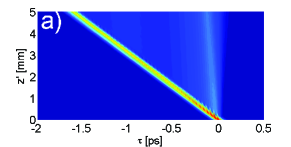
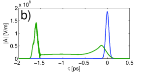
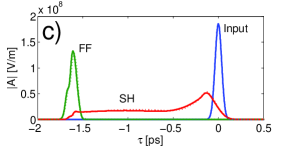
Figure 1: Propagation of a femtosecond pulse in a PPLT crystal. a) Evolution of the field amplitude $|A|$ from numerical solution of Eq. (Nonlinear envelope equation for broadband optical pulses in quadratic media). b) Electric field amplitude at the crystal output. c) Comparison between coupled wave solution (dotted curves) and $|A|$ filtered around fundamental and second harmonic (solid curves). The initial pulse has gaussian shape and the parameters are $T=60fs$, $I=10GW/cm^{2}$, $\lambda_{in}=1400nm$, $\lambda_{0}=2\pi c/\omega_{0}=700nm$, $d_{33}=\chi_{LT}^{(2)}/2=10.6pm/V$

In order to show the validity of our equation, we simulated the propagation of a femtosecond pulse in a $L=5mm$ long periodically poled lithium tantalate sample (PPLT). To model the refractive index dispersion we employed a Sellmeier model fitted from experimental data neslt and nonlinear coefficient is $d_{33}=\chi_{LT}^{(2)}/2=10.6pm/V$. In the numerical code we inserted the exact dispersion relation $k(\omega)$. We assumed a first order quasi phase matching (QPM) grating, with a period $\Lambda=17.4\mu m$. We thus allowed a periodic variation of the nonlinear coefficent $\chi^{(2)}$=$\chi^{(2)}(z)=2/\pi\chi^{(2)}_{LT}e^{i2\pi/\Lambda z}$+c.c.. We injected a $T=60fs$ FWHM long gaussian pulse, centered around $1400nm$, with $I=10GW/cm^{2}$ peak intensity. The corresponding residual phase mismatch is $\Delta k=2k(\omega_{in})-k(2\omega_{in})=10000m^{-1}$, where $\omega_{in}$ is the carrier frequency of the input pulse. In the simulation we set the reference frequency $\omega_{0}$ to be equal to the second harmonic of the input pulse: in this way the second harmonic is stationary in the reference frame $(z^{\prime},\tau)$.
Figure 1a) shows the evolution of the electric field envelope amplitude $|A|$ from numerical solution of Eq. (Nonlinear envelope equation for broadband optical pulses in quadratic media). We can see the typical scenario of the propagation of femtosecond pulses in highly group velocity mismatched (GVM) process: the fundamental frequency (FF) pulse generates its second harmonic (SH) during propagation, and the generated SH pulse has the typical shape of a initial peak followed by a long tail, whose duration is fixed by the product between GVM and crystal length. Figure 1b) shows the electric field envelope amplitude at the end of the crystal. It can be seen a peak that corresponds to the faster frequency components located around FF, followed by a long tail that ends with a second lower peak. This long pulse corresponds to the generated SH components. The SH pulse is smooth, indicating that no beating with eventual FF components is present. Whereas in the residual FF pulses centered around $\tau\approx-1.6ps$, there is a clear fast oscillation, indicating that FF and SH components are superimposed.
To test the results, we simulated the same set-up with a standard coupled wave model Conforti07 , by inserting the values of first and second order dispersion evaluated at FF and SH. To compare the results we filtered $A$ around FF and SH. Figure 1c) shows the electric field amplitudes at the end of the crystal. The results of the two models are practically indistinguishable. It is worth noting that this simulation shows the validity of Eq. (Nonlinear envelope equation for broadband optical pulses in quadratic media) over a bandwidth of $\omega_{0}$.

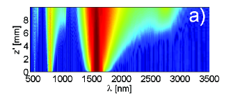
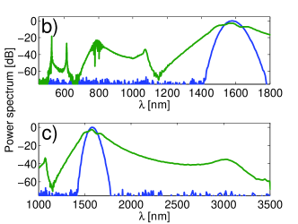
Figure 2: Propagation of a femtosecond pulse into a PPLN sample. a) Evolution of the power spectrum (in dB) from numerical solution of Eq. (Nonlinear envelope equation for broadband optical pulses in quadratic media). b) Power specrum at the crystal output in the visible and NIR range. c) Power specrum at the crystal output in the infrared range. The division into separate spectral region is made to facilitate the comparison with experimental data Langrock07 . The initial pulse has gaussian shape and the parameters are $T=50fs$, $I=15GW/cm^{2}$, $\lambda_{in}=1580nm$, $\lambda_{0}=2\pi c/\omega_{0}=700nm$, $d_{33}=\chi_{LN}^{(2)}/2=27pm/V$

As a second example we consider the propagation of a femtosecond pulse into a highly mismatched periodically poled lithium niobate (PPLN) sample, that was demonstrated experimentally to generate an octave spanning supercontinuum spectral broadening Langrock07 . To model the refractive index dispersion we employed a Sellmeier model fitted from experimental data jundt and nonlinear coefficient is $d_{33}=\chi_{LN}^{(2)}/2=27pm/V$. In the numerical code we inserted the exact dispersion relation $k(\omega)$. We assumed a QPM grating with a period $\Lambda=30\mu m$ (phase matched for second harmonic generation at around $2\mu m$ fundamental wavelength). We included higher order QPM terms, since the huge bandwidth can phase match different spatial harmonics. We injected a $T=50fs$ FWHM long gaussian pulse, centered around $1580nm$, with $I=15GW/cm^{2}$ peak intensity. In the simulation we set the reference wavelength $\lambda_{0}=700nm$. Figure 2a) shows the evolution of the spectrum during the propagation into a $L=7mm$ crystal. We can see a consistent broadening and redshift of the FF part of the spectrum that, at the end of the crystal, reaches an octave-spanning bandwidth from $1200nm$ to $3000nm$. We can also see the generation of spectral components at the second and third harmonics. At the second harmonic the spectrum initially broadens and has an evolution ruled by highly mismatched SHG. When the FF broadening reaches the first order quasi phase matching wavelength at around $2\mu m$, the more efficient conversion process generates a spike at around $1\mu m$. Figure 2 b) shows the visible and the near infrared (NIR) part of the spectrum at the crystal output. We can see a broadband second and third harmonic of the broadened laser spectrum, and the presence of some spikes given by the quasi phase matching of high order spatial harmonics of the grating. We verified that the two spikes at the third harmonic correspond to the third and fifth order QPM for the process $\omega+2\omega\rightarrow 3\omega$. We can also see a spectral overlap between the harmonics of the broadened laser spectrum, that can be exploited to achieve carrier-envelope-offset phase slip stabilization Langrock07 , that is of paramount importance for frequency metrology applications.
Figure 2c) shows the infrared spectrum at the output. This spectrum exhibits more than an octave spanning between $1300nm$ and $3000nm$ at the $-40dB$ spectral power lever with respect to the peak power level. The spectral components near the zero GVM wavelength around $3000nm$ are generated more efficiently.
All the features described above compares surprisingly well with the experimental results of Langrock et al. Langrock07 , even if we simulate a slightly different environment. In fact we use a bulk PPLN sample and not a RPE PPLN waveguide. The effect of waveguide is to slightly modify the power levels and the crystal dispersion: a detailed simulation of the real set-up is out of the scope of this Letter. It is worth noting that numerical modelling of such phenomena without our model is an irksome job since (i) time domain Maxwell equation solvers require a prohibitive computational effort and (ii) coupled wave approaches cannot be used in the presence of overlapping among frequency bands of different field components.

In conclusion we have derived a robust nonlinear envelope equation describing the propagation in dispersive quadratic materials. Thanks to a proper formal definition of the complex envelope, it is possible to treat pulses of arbitrary frequency content. A proper definition of envelope is crucial for second order nonlinearities, due to the generation of frequency components around zero. Computationally it is possible to accurately evolve optical pulses of arbitrarily wide band over a meter scale physical distance, which is a few order of magnitude longer than those accessible by Maxwell equation solvers.

References

- (1) R. W. Boyd, Nonlinear Optics, (Academic Press, 2003), 2nd ed.
- (2) T. Brabec and F. Krausz, Phys. Rev. Lett. 78, 3282 (1997).
- (3) T. Brabec and F. Krausz, Rev. Mod. Phys. 72, 545 (2000).
- (4) M. Geissler et al., Phys. Rev. Lett. 83, 2930 (1999).
- (5) A. V. Husakou and J. Herrmann, Phys. Rev. Lett. 87, 203901 (2001).
- (6) M. Kolesik, J. V. Moloney and M. Mlejnek, Phys. Rev. Lett. 89, 283902 (2002).
- (7) G. Genty, P. Kinsler, B. Kibler and J. M. Dudley, Opt. Express 15, 5382 (2007).
- (8) P. Kinsler and G. H. C. New, Phys. Rev. A 67, 023813 (2003).
- (9) J. Moses and F. W. Wise, Phys. Rev. Lett 97, 073903 (2006).
- (10) C. Langrock, M. M. Fejer, I. Hartl, and M. E. Fermann, Opt. Lett. 32, 2478 (2007).
- (11) S. Haykin, Communication System, (John Wiley & Sons, 2001), 4th ed.
- (12) A. Bruner et al., Opt. Lett. 28, 194 (2003).
- (13) M. Conforti, F. Baronio, and C. De Angelis, Opt. Lett. 32, 1779 (2007).
- (14) D. H. Jundt, Opt. Lett. 22, 1553 (1997).