Variational quantum tomography with incomplete information by means of semidefinite programs

Abstract

We introduce a new method to reconstruct unknown quantum states out of incomplete and noisy information. The method is a linear convex optimization problem, therefore with a unique minimum, which can be efficiently solved with Semidefinite Programs. Numerical simulations indicate that the estimated state does not overestimate purity, and neither the expectation value of optimal entanglement witnesses. The convergence properties of the method are similar to compressed sensing approaches, in the sense that, in order to reconstruct low rank states, it needs just a fraction of the effort correspondig to an informationally complete measurement.

I Introduction

All we can know about a quantum system can be compactly represented by its state or density matrix, i.e., a trace one positive operator ($\rho$). The observable properties of the system are represented by Hermitian operators ($O$), and their expectation values are given by the rule: $Tr(\rho O)$. Consider the system is defined on a Hilbert space of dimension $d$. In this case, the state ($\rho$) is a $d\times d$ Hermitian matrix, or a real $d^{2}$ dimensional vector in the Hilbert-Schmidt space. As the state is normalized ($Tr(\rho)=1$), it has just $d^{2}-1$ independent real parameters, so it is in fact a $d^{2}-1$ dimensional real vector. Therefore, a carefully chosen set of $d^{2}-1$ independent measurements, in the sense that it forms a complete basis in the Hilbert-Schmidt space, allows for the reconstruction of the state. This approach is usually referred to as quantum tomography.

There are many methods to estimate a quantum state (for a review, see, for example, QSE ). An important class of these methods is known as maximum-likelihood quantum tomography (MaxLik) (see, for example, ML0 ; ML1 ; ML2 ; ML3 ). MaxLik is a statistical inference approach which yields probability distributions as close as possible to the measured frequencies. Nonetheless, these probability distributions frequently correspond to non-positive operators, due to the always present experimental imprecisions. It is important to stress that our method does not follow this line. Our heuristic consists of performing a variational search in the state space for the best trace one positive operator compatible with the measured data. Note also that MaxLik cannot guarantee that fake entanglement be not attributed to the system Horodecki . Our numerical simulations indicate that the method we propose does not overestimate entanglement. Another important aspect of our method is that it can be solved exactly, for it can be cast as a linear convex optimization problem, while the usual algorithms for quantum state tomography, though convex, are non-linear, and the actual algorithms implementing them can be plagued with many local minima.

To perform the complete set of measurements necessary to reconstruct the quantum state of a moderately sized system could be impossible in practice. As an example, consider the experimental generation of the 8-qubit entangled state reported by Häffner et al. Blatt . To tomograph the 8-qubit system, 65536 projectors needed to be measured ($2^{16}$), and the computational effort to apply MaxLik to such a state is discouraging, though it was done. But the tomography of a larger system could be inaccessible experimentally, and yet we would like to assess its properties. The exponential growth of the Hilbert space is insurmountable, in this respect. Using the Maximum Entropy Inference Principle of Jaynes Jaynes (MaxEnt), one can estimate a quantum state out of incomplete information. In this approach, one searches for the maximum entropy state, compatible with the measured data Buzek . This state corresponds to maximum ignorance with respect to the unmeasured set of observables forming the complete basis for the density operator. The Horodecki Horodecki showed an example where the direct application of MaxEnt yielded fake entanglement, i.e., the reconstructed state was entangled, while the available data were compatible with a non-entangled state. Our method can also estimate a state out of incomplete information, and with the advantage of not overstimating entanglement, as indicated by our simulations.

Another interesting aspect of our method is that it can identify incompatible data. Suppose a set of complete measurements are being performed, aiming a quantum state reconstruction. It can happen that, for a particular complete measurement, some parameters of the experimental setup have fluctuated to a point of changing the quantum state, but it went unnoticed by the experimentalist. In this case, data for different states have been collected. When our method is applied to these measurements, the algorithm will detect that the data are incompatible with a single quantum state. Then some of the data can be discarded, and the state can be reconstructed.

In the next section, we develop a variational method to estimate a state, which relies on incomplete and noisy information of the quantum state. The method we obtain has the particular form of a linear convex optimization problem, known as Semidefinite Program (SDP), for which efficient and stable algorithms are available Boyd ; sedumi ; yalmip . Though this unfortunate name can suggest a kind of black-box computational algorithm, a SDP is not so. It consists of minimizing a linear objective under a linear matrix inequality constraint, precisely,

minimize $c^{\dagger}x$

$$subject\,\,to\left\{F(x)=F_{0}+\sum_{i=1}^{m}x_{i}F_{i}\geq 0,\right.$$ (1)

where $c\in C^{m}$ and the Hermitian matrices $F_{i}\in C^{n\times n}$ are given, and $x\in C^{m}$ is the vector of optimization variables. $F(x)\geq 0$ means that $F(x)$ is a positive matrix. The problem defined in Eq.1 has no local minima. When the unique minimum of this problem cannot be found analytically, one can resort to powerful algorithms that return the exact answer sedumi . To solve the problem in Eq.1 could be compared to finding the eigenvalues of a Hermitian matrix. If the matrix is small enough or has very high symmetry, one can easily determine its eigenvalues, but in other cases some numerical algorithm is needed. Anyway, one never doubts that the eigenvalues of such a matrix can be determined exactly. We point out that we have successfully used SDPs before, in the development of powerful methods to construct entanglement witnesses rov1 ; rov2 ; rov4 ; rov3 .

After discussing the methodology, we present a section with numerical examples that we consider representative, namely, a full rank highly symmetric two-qutrit density matrix, and a pure (rank one) five-qubit state. Our method works equally well in these two extreme cases. Then we show reconstruction of four-qubit mixed states of all ranks, in order to have a better taste of the convergence properties of our method. These numerical examples suggest that our method converges very fast for low rank states, or for states that, though of high rank, have very high symmetry. These convergence properties are similar to recent introduced approaches in compressed sensing Eisert . To reconstruct, with high fidelity, full rank states with no symmetry, an informationally complete measurement is needed. But even in these difficult cases, our method can yield reasonable lower bounds to entanglement out of incomplete information rov3 . We illustrate this feature by evaluating optimal entanglement witnesses rov1 ; rov2 ; rov4 ; rov3 in qubit-qutrit full rank states, with increasing number of measurements. Besides the numerical examples, we have also successfully tested our approach in a real experiment, where entangled qutrits were generated in a quantum optics setup Lima .

II Theory

The state of a quantum system is represented by its density matrix $\rho$, which is a $d^{2}-1$ dimensional real vector in the Hilbert-Schmidt space. Therefore, we can write it as:

$$\rho=C_{0}I+\sum_{l=1}^{d+1}\sum_{i=1}^{d-1}C_{il}P_{i}^{l}=C_{0}I+\sum_{\lambda=1}^{d^{2}-1}C_{\lambda}P_{\lambda},$$ (2)

where the $P_{i}^{l}=P_{\lambda}$ are Hermitian operators, forming a complete basis in the Hilbert-Schmidt space, $I$ is the identity, and $\lambda$ is just a convenient compact index.

Now, for concreteness, we assume the operators in each class $l$ are rank one projectors, forming a complete measurement, i.e.,

$$\begin{array}[]{l}I=\displaystyle{\sum_{i=1}^{d}}P_{i}^{l},\\ \\ Tr(P_{i}^{l}P_{j}^{l})=\delta_{ij}.\end{array}$$ (3)

$C_{0}$, which is not an independent parameter, in this case is given by $C_{0}=(1-\sum_{\lambda=1}^{d^{2}-1}C_{\lambda})/d$. Note that, in Eq.2, we use just $d-1$ projectors from each complete measurement labelled by $l$ (for the $d$ probabilities sum to one). Besides being convenient for our calculations, this basis also has the minimum number of projectors necessary to expand a Hermitian matrix with fixed trace, but the method we derive is not basis dependent. For instance, if one chooses to expand the state in a SU basis, like a generalized Bloch representation,

$$\rho=\frac{1}{d}I+\sum_{i=1}^{d^{2}-1}r_{i}\sigma_{i}\,,$$ (4)

to obtain the coefficients $r_{i}=Tr(\rho\sigma_{i})$, one should consider the spectral decomposition $\sigma_{i}=\sum_{j=1}^{d}\alpha_{ij}|i_{j}\rangle\langle i_{j}|$, and we are back to the measurement of projectors, $Tr(|i_{j}\rangle\langle i_{j}|\rho)$. But now, instead of the $d^{2}-1$ projectors of Eq.2, one has $d\times(d^{2}-1)$ projectors, i.e., one complete measurement for each operator $\sigma_{i}$. The use of POVMs (Positive Operator Valued Measure) also poses no difficulties, for it consists of measurements of rank one projectors again.

We assume that from a set of $d^{2}-1$ projectors (or observables), forming a complete basis in the Hilbert-Schmidt space (the space of linear operators), just $N(<d^{2}-1)$ have been measured. We refer to measured and unmeasured projectors (observables) as the known and unknown sets, respectively. Now we introduce the following cost operator (the sum of the projectors in the unknown set), which can be thought of as a Hamiltonian:

$$H=\sum_{\lambda=N+1}^{d^{2}-1}P_{\lambda}.$$ (5)

We want a trace one positive operator, which minimizes the cost function:

$$E=Tr(H\tilde{\varrho})=\sum_{\lambda=N+1}^{d^{2}-1}q_{\lambda},$$ (6)

where $q_{\lambda}$ are positive numbers corresponding to the projections of $\tilde{\varrho}$ on the unknown set. Our variational principle now reads:

$$\delta E=Tr(H\delta\tilde{\varrho})=0.$$ (7)

The Lagrangian for this problem reads:

$$\begin{array}[]{ll}L=&E+\alpha[Tr(\tilde{\varrho})-1]+\displaystyle{\sum_{\lambda=1}^{N}}\beta_{\lambda}[Tr(\tilde{\varrho}P_{\lambda})-p_{\lambda}]+\\ &\displaystyle{\sum_{\lambda=N+1}^{d^{2}-1}}\gamma_{\lambda}[Tr(\tilde{\varrho}P_{\lambda})-q_{\lambda}],\end{array}$$ (8)

where $\alpha$, $\beta_{\lambda}$, and $\gamma_{\lambda}$ are Lagrange multipliers corresponding to the constraints on the quantum state.

Eq.2 in matrix form reads

$$\rho=C^{T}P,$$ (9)

where $C$ is a column vector with the real coefficients $C_{\lambda}$, and $P$ a column vector collecting the matrices $P_{\lambda}$. Consider the overlap matrix $S$, with elements $S_{\mu\nu}=Tr(P_{\mu}P_{\nu})$, and the column vector $\mathcal{P}$, with elements $p_{\lambda}=Tr(\rho P_{\lambda})$. Then we have

$$C=S^{-1}\mathcal{P}.$$ (10)

Only when the probabilities in $\mathcal{P}$ are exact, the vector $C$ yields a positive operator, by means of Eq.9. But it is never the case, in practice. The frequencies obtained from an experiment are noisy, thus:

$$Tr(\rho P_{\lambda})\in[p_{\lambda}-\varepsilon,p_{\lambda}+\varepsilon],$$ (11)

with $\varepsilon$ positive, and hopefully small.

To account for Eq.11 in our algorithm, we introduce the additional constraints:

$$\begin{array}[]{l}Tr(\tilde{\varrho}P_{\lambda})\geq(1-\Delta_{\lambda})p_{\lambda},\\ Tr(\tilde{\varrho}P_{\lambda})\leq(1+\Delta_{\lambda})p_{\lambda},\\ \Delta_{\lambda}\geq 0,\,\,\,\lambda\in[1,N].\end{array}$$ (12)

Again, we want to determine a trace one positive operator $\tilde{\varrho}$, with minimum $\Delta_{\lambda}$. It is important to note that Eq.12 is not to be interpreted as any kind of statistical treatment. By minimizing $\Delta_{\lambda}$, we are simply adjusting the frequencies obtained in the laboratory, such that we get a positive matrix by means of Eqs.9 and 10. This works only when Eq.11 is valid for all frequencies. If some frequencies came from another state, say $Tr(\rho_{other}P_{\lambda})$, then the algorithm will diverge, and we have identified incompatible data. To build an appropriate Lagrangian for this problem, we introduce positive numbers $v_{\lambda}$ and $w_{\lambda}$, which should be minimized, and rewrite Eq.12 as:

$$\begin{array}[]{l}Tr(\tilde{\varrho}P_{\lambda})-(1-\Delta_{\lambda})p_{\lambda}=v_{\lambda},\\ (1+\Delta_{\lambda})p_{\lambda}-Tr(\tilde{\varrho}P_{\lambda})=w_{\lambda}.\end{array}$$ (13)

The Lagrangian now reads:

$$\begin{array}[]{ll}L=&E+\displaystyle{\sum_{\lambda=1}^{N}}(\Delta_{\lambda}+v_{\lambda}+w_{\lambda})+\alpha[Tr(\tilde{\varrho})-1]+\\ &\displaystyle{\sum_{\lambda=N+1}^{d^{2}-1}}\gamma_{\lambda}[Tr(\tilde{\varrho}P_{\lambda})-q_{\lambda}]+\\ &\displaystyle{\sum_{\lambda=1}^{N}}\{\zeta_{\lambda}[(1+\Delta_{\lambda})p_{\lambda}-Tr(\tilde{\varrho}P_{\lambda})-w_{\lambda}]+\\ &\eta_{\lambda}[Tr(\tilde{\varrho}P_{\lambda})-(1-\Delta_{\lambda})p_{\lambda}-v_{\lambda}]\},\end{array}$$ (14)

where $\zeta_{\lambda}$ and $\eta_{\lambda}$ are additional Lagrange multipliers. Note that this Lagrangian defines a convex problem. We want to minimize a linear function, constrained by matrix inequalities. Our variable is $\tilde{\varrho}$, and the search space is restricted to the cone of positive matrices. This is a typical convex optimization problem, known as Semidefinite Program (SDP), as described in the Introduction (Eq.1). SDPs have a unique minimum, and can be solved very efficiently Boyd . Our SDP reads:

minimize $(E+\sum_{\lambda=1}^{N}\Delta_{\lambda})$

$$subject\,\,to\left\{\begin{array}[]{l}\tilde{\varrho}\geq 0,\\ Tr(\tilde{\varrho})=1,\\ \Delta_{\lambda}\geq 0,\\ Tr(\tilde{\varrho}P_{\lambda})\geq(1-\Delta_{\lambda})p_{\lambda},\\ Tr(\tilde{\varrho}P_{\lambda})\leq(1+\Delta_{\lambda})p_{\lambda},\,\,\,\forall\lambda\in[1,N]\,.\end{array}\right.$$ (15)

Now we have concluded the derivation of our method. Eq.15 returns a state $\tilde{\varrho}$ which is the optimal approximation to the unknown state $\rho$.

III Applications

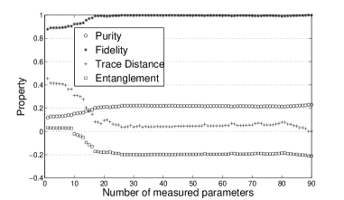
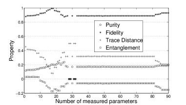
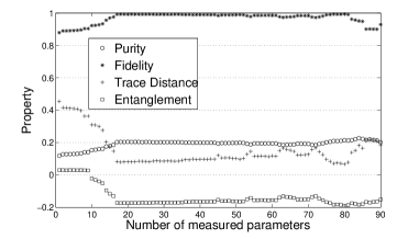
Figure 1: Estimation of some properties and reconstruction of a two-qutrit full rank Werner state ($\beta=-0.8$, cf. Eq.16). We plot Purity, $Tr(\tilde{\varrho}^{2})$, Fidelity, $Tr(\sqrt{\rho^{\frac{1}{2}}\tilde{\varrho}\rho^{\frac{1}{2}}})$, Trace Distance, $\frac{1}{2}Tr|\tilde{\varrho}-\rho|$, and entanglement, $Tr(W_{\tilde{\varrho}}\tilde{\varrho})$ ($W_{\tilde{\varrho}}$ is the trace-one optimal entanglement witness), against the number of measured projectors. The measurements have statistical errors of up to 50%, according to a uniform distribution. In the last two panels, we introduced measurements from another Werner state ($\beta=+0.8$), to show that the algorithm is capable to identify incompatible data (see text for details).

Figure 2: Reconstruction of a five-qubit low entangled pure state. We plot Purity, $Tr(\tilde{\varrho}^{2})$, Fidelity, $Tr(\sqrt{\rho^{\frac{1}{2}}\tilde{\varrho}\rho^{\frac{1}{2}}})$, Trace Distance, $\frac{1}{2}Tr|\tilde{\varrho}-\rho|$, and entanglement, $Tr(W_{\tilde{\varrho}}\tilde{\varrho})$ ($W_{\tilde{\varrho}}$ is the trace-one optimal entanglement witness), against the number of measured projectors. Note that the exact state is recovered with just 160 measurements out of the total of 1056, that would be necessary to completely span the Hilbert-Schmidt space.

Now we would like to illustrate the use of Eq.15. As the examples show, our method does not overestimate purity and neither the expectation value of optimal entanglement witnesses rov1 ; rov2 ; rov4 ; rov3 , and it can also identify incompatible data. The examples also show that few measurements are needed to reconstruct both low rank states, and full rank states with high symmetry (Figs. 1, 2 and 3). In Figs. 1, 2 and 3, the set of measurements we chose for the state expansion is mutually unbiased bases (MUB) Ivanovic ; Wootters , in the sense that any two vectors of different complete measurements have the same overlap’s absolute value. As demonstrated by Wootters et. al Wootters and Ivanovic Ivanovic , this is the best informationally complete projective measurement one can do. It is optimal both in the statistical sense and in the number of projectors to be measured. The POVMs that would be equivalent to MUBs are the Symmetrically Informationally Complete POVMs (SIC-POVM) povm . But while the MUBs are known for all Hilbert spaces which have dimension of power of a prime, SIC-POVMs, though conjectured to exist in all dimensions, are known just in a few particular cases. In Fig. 4, we used the SU(6) basis, to illustrate that our method works with any kind of basis.

Our first example is a highly mixed 2-qutrit Werner state Werner (purity=0.23), which is full rank, and has entanglement -0.21, according to its optimal trace one entanglement witness rov1 ; rov2 . The explicit expression of this state is:

$$\rho=\frac{I+\beta F}{9+3\beta},$$ (16)

with $-1\leq\beta\leq 1$. $\rho$ is separable for $\beta\geq-\frac{1}{3}$. $F$ is a swap operator for two qutrits,

$$F=\sum_{i,j=1}^{3}|ij\rangle\langle ji|.$$ (17)

For two qutrits, we have ten complete measurements, with nine projectors in each one. In Fig.1, we plot, against the number of measured projectors, purity, fidelity and trace distance to the true or exact state, and the witnessed entanglement ($Tr(W_{\tilde{\varrho}}\tilde{\varrho})$ - the more negative is this expectation value, the more entangled is the state). In the calculations of entanglement, we use an optimal trace one witness, obtained with techniques developed in rov1 ; rov2 ; rov4 ; rov3 . The optimal entanglement witness has to be calculated for each state individually. The (simulated) measured frequencies (Eq.11) have statistical errors of up to 50%, according to a random uniform distribution. In the first panel, one can see that with about twenty measurements, from a total of ninety, we have a practically perfect estimation of the entanglement, and the state was reconstructed with high fidelity, or low trace distance. Note that all the properties we are calculating converge monotonically, never been overestimated. In the second panel, the third complete measurement (indexed 19 to 27) corresponds to a different Werner state. Note that we had convergence up to the $18^{th}$ projection, and then all the properties started to diverge, to resume convergence again in the fourth measurement. In the last panel, the incompatible data was moved to positions 81 to 90, and one can see convergence for the measurements before this. The fluctuations seen in all the panels are due to the large statistical errors we imposed, added to the fact that without all the complete measurements, there is always the possibility of a family of close states to fit the data.

To highlight the efficiency of our method, in Fig.2 we applied it to a a five-qubit low entangled pure state (it is a normalized random vector with 32 complex coefficients). In principle, one needs to perform 33 complete measurements (1056 projectors) to reconstruct such a state, but we needed just five (160 projectors). The entanglement plotted in the figure is the genuine five-party one, given by the trace one optimal entanglement witness rov1 ; rov2 ; rov4 ; rov3 . The tomography calculation took six seconds in a laptop, with a 2.8GHz processor, and 3GB of RAM, running MATLAB under Linux. The five-party entanglement calculation was more expensive, and took about forty minutes.

Fig.3 illustrates the convergence properties of our method, as the rank of the density matrices increases. For a system of four qubits (Hilbert-Schmidt space dimension of 256), we consider one hundred random density matrices of each rank, varying from pure states (rank one) to full rank states (rank 16). We plot the average number of measurements to reconstruct the state with high fidelity ($Tr|\rho-\tilde{\varrho}|<10^{-6}$), against the rank. In the figure we also indicate the minimum (Best Case) and maximum (Worst Case) number of measurements needed in the reconstruction, in each sample. We see that the state reconstruction needs very few measurements for low rank states, and it can need all the measurements for high rank states. This behavior is similar to the compressed sensing approach reported in Eisert .

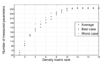
Figure 3: Reconstruction of random four-qubit entangled states of all ranks. The average number of measurements needed to a highly faithful reconstruction ($Tr|\rho-\tilde{\varrho}|<10^{-6}$) is plotted against the rank of the state. For each rank, it is employed a sample of one hundred states. For each sample, it is also plotted the minimum (Best Case) and maximum (Worst Case) number of measurements needed.

As a last example, we consider a qubit-qutrit system. The states will be expanded in the 36 SU(6) observables ($\sigma_{i}$) forming an informationally complete basis in the Hilbert-Schmidt space (cf. Eq.4). The Hamiltonian (cf. Eq.5) to be used in Eq.15 is formed by the eigenprojectors of the $36-N$ unmeasured $\sigma_{i}$ (cf. Eq.4). For $10^{3}$ random full-rank density matrices ($\rho_{i}$), we plot, against the number of measured observables, the average trace distance ($10^{-3}\sum_{i=1}^{1000}Tr|\tilde{\varrho_{i}}-\rho_{i}|/2$), and average fraction of entanglement, defined as follows. The entanglement of a state is $E(\rho)=Tr(W_{\rho}\rho)$, if this expectation value is negative, and zero otherwise. $W_{\rho}$ is the optimal trace one entanglement witness for the state $\rho$, calculated with the techniques described in rov1 ; rov2 ; rov4 ; rov3 . Thus, the Entanglement plotted in the figure is given by $10^{-3}\sum_{i=1}^{1000}E(\tilde{\varrho_{i}})/E(\rho_{i})$. The full rank states will need all the 36 measurements to be reconstructed with high fidelity, for they have no symmetry. Even though, Fig.4 shows that a non null lower bound to the entanglement is obtained with less measurements, and of course this bound tends to the correct entanglement as the number of measurements increases.

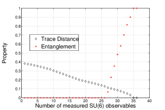
Figure 4: Reconstruction of $10^{3}$ full rank random qubit-qutrit entangled states. We plot the fraction of the true entanglement, on average, as the number of measurements increases (see text for details). The average trace distance to the true state is also plotted. We see that an almost perfect reconstruction is possible only with all the measurements, but non null lower bounds to the entanglement are obtained with less measurements.

IV Conclusion

We developed a method that yields an estimate ($\tilde{\varrho}$) of a unknown quantum state ($\rho$), without the need to perform an informationally complete measurement. Our numerical simulations indicate that our method does not overestimate entanglemnt, and does not underestimate purity. These quantities tend to the true values, as the number of measurements increases towards an informationally complete measurement. Low rank states, or high rank states with high symmetry can be reconstructed with high fidelity, using few measurements. This is simply because the number of independent parameters in such density matrices is much less than $d^{2}$, the dimension of the Hilbert-Schmidt space. Note that it is a line of investigation we started in rov3 , in the context of entanglement detection with few measurements. The method can be useful in the study of larger systems, where an informationally complete measurement is out of question. In this respect, we note that the convergence properties of our method is similar to the compressed sensing approach recently introduced in Eisert .

We conclude by mentioning that our method has been successfully employed in a real experiment reported in Lima . We also mention that we have extended our method to the problem of process tomography processo .

Acknowledgments - We thank C.H. Monken, S.P. Walborn and P.H Souto Ribeiro for the discussions. We also acknowledge Fernando G.S.L. Brandão and the referee for pointing out a mistake, in the manuscript, concerning lower bounds of expectation values.

Financial support by the Brazilian agencies FAPEMIG, and INCT-IQ (National Institute of Science and Technology for Quantum Information).

References

- (1) M. Paris, J. Rehacek (Eds), Quantum State Estimation., Lect. Notes Phys. 649 (Springer, Berlin Heidelberg 2004), DOI 10.1007/b98673.
- (2) Z. Hradil, J. Rehacek, J. Fiurasek, M. Jezek, “Maximum-Likelihood Methods in Quantum Mechanics”, in M. Paris, J. Rehacek (Eds), Quantum State Estimation., Lect. Notes Phys. 649 (Springer, Berlin Heidelberg 2004), DOI 10.1007/b98673, pp. 59-100.
- (3) G.M. D’Ariano, D.F. Magnani, P. Perinotti, Phys. Lett. A, 373, 111-115 (2009).
- (4) G.M. D’Ariano, P. Perinotti, P., Phys. Rev. Lett., 98, 020403 (2007).
- (5) J. Rehacek, Z. Hradil, E. Knill, A.I. Lvovsky, Phys. Rev. A, 75, 042108 (2007).
- (6) R. Horodecki, M. Horodecki, P. Horodecki, Phys. Rev. A, 59, 1799-1803 (1999).
- (7) E.T. Jaynes, Phys. Rev. 106, 620-630 (1957).
- (8) V. Buzek, “Quantum Tomography from Incomplete Data via MaxEnt Principle”, in M. Paris, J. Rehacek (Eds), Quantum State Estimation., Lect. Notes Phys. 649 (Springer, Berlin Heidelberg 2004), DOI 10.1007/b98673, pp. 189-230.
- (9) H. Häffner, W. Hänsel, C.F. Roos, J. Benhelm, D. Chek-al-kar, M. Chwalla, T. Körber, U.D. Rapol, M. Riebe, P.O. Schmidt, C. Becher, O. Gühne, W. Dür, R. Blatt, Nature, 438, 643-646 (2005).
- (10) S. Boyd, L. Vandenberghe, Convex Optimization, (Cambridge University Press, Cambridge, 2000).
-
(11)
J.F. Sturm, Optim. Methods and Software 11,
625-653 (1999);
SEDUMI: http://fewcal.kub.nl/sturm/softwares/sedumi.html. - (12) J. Löfberg, YALMIP : A Toolbox for Modeling and Optimization in MATLAB, Proceedings of the CACSD Conference, 2004, Taipei, Taiwan, (unpublished) http://control.ee.ethz.ch/~joloef/yalmip.php.
- (13) F.G.S.L Brandão, and R.O. Vianna, Phys. Rev. Lett. 93, 220503 (2004).
- (14) F.G.S.L. Brandão, and R.O. Vianna, R.O., Int. J. Quantum Inf. 4, 331-340 (2006).
- (15) F.G.S.L. Brandão, and R.O. Vianna, Phys. Rev. A, 70, 062309 (2004).
- (16) T.O. Maciel, and R.O. Vianna, Phys. Rev. A, 80, 032325 (2009).
- (17) D. Gross, Y. Liu, T. Flammia, T., S. Becker, J. Eisert, Phys. Rev. Lett. 105, 150401 (2010).
- (18) G. Lima, E.S Gómez, A. Vargas, R. O. Vianna, and C. Saavedra, Phys. Rev. A, 82, 012302 (2010).
- (19) R.F. Werner, Phys. Rev. A 40, 4277-4281 (1989).
- (20) I.D. Ivanovic, J. Phys. A: Math. Gen. 14, 3241 (1981).
- (21) W.K. Wootters, B.D. Fields, Ann. Phys. 191, 363-381(1989).
- (22) J. K. Renes, R. Blume-Kohout, A. J. Soctt, C. M. Caves, J. Math. Phys. 45, 2171 (2004).
- (23) T.O. Maciel and R.O. Vianna, Optimal estimation of quantum processes using incomplete information: variational quantum process tomography, arXiv:1007.2395.