Channel Capacities of an Exactly Solvable Spin-Star System

Abstract

We calculate the entanglement-assisted and unassisted channel capacities of an exactly solvable spin star system, which models the quantum dephasing channel. The capacities for this non-Markovian model exhibit a strong dependence on the coupling strengths of the bath spins with the system, the bath temperature, and the number of bath spins. For equal couplings and bath frequencies, the channel becomes periodically noiseless.

I Introduction

One of the fundamental tasks of quantum information theory is to determine the information transmission capacities of quantum channels Bennett and Shor (1998); Nielsen and Chuang (2000). The maximum amount of information that can be reliably transmitted over a channel, per channel use is known as its capacity Cover and Thomas (1991). Classical channels can be uniquely characterized by their capacity Shannon (1948). The situation in the quantum realm is significantly more involved, with various capacities required to characterize a quantum channel Bennett and Shor (2004).

Studies of quantum channel capacities can be broadly divided into those considering memoryless quantum channels, for which the output at a given time depends only upon the corresponding input and not upon any previous inputs Hausladen et al. (1996); Schumacher and Westmoreland (1997); Lloyd (1997); Bennett et al. (1997); Adami and Cerf (1997); Barnum et al. (1998); Bennett et al. (1999, 2002); Shor (2002); Holevo (2002); Liang (2002); Daffer et al. (2003); Shor (2004a); Kretschmann and Werner (2004); Devetak (2005); Giovannetti and Fazio (2005); Wolf and Pérez-García (2007), and quantum memory channels, where successive uses of the channel modify its properties and description Macchiavello and Palma (2002); Yeo and Skeen (2003); Macchiavello et al. (2004); Bowen and Mancini (2004); Arshed and Toor (2006); D’Arrigo et al. (2007); Plenio and Virmani (2007); Bayat et al. (2008). Another important distinction is between channels generated by Markovian vs. non-Markovian environments or baths. Markovian channels describe memoryless baths, while for non-Markovian channels bath memory plays a role H.-P. Breuer and F. Petruccione (2002); Breuer et al. (2009). Many quantum optical Carmichael (1993) and nuclear magnetic resonance systems Slichter (1996) are accurately described by Markovian channels, but the Markovian limit is always an approximation R. Alicki, D. A. Lidar, and P. Zanardi (2006). Non-Markovian effects are especially important in condensed matter systems, such as coupled electron or nuclear spins U. Weiss (1993). The master equations describing the dynamics of non-Markovian systems are often (though not always A. Shabani and D. A. Lidar (2005)) complicated integro-differential equations which are rarely exactly solvable H.-P. Breuer and F. Petruccione (2002). A channel can be memoryless yet non-Markovian. This situation arises when successive uses do not modify the channel, but a proper description of each use of the channel requires a non-Markovian treatment accounting for bath memory effects. In this work we investigate how non-Markovian effects modify channel capacities by studying an exactly solvable model of a non-Markovian memoryless channel: the Ising spin-star system H. Krovi, O. Oreshkov, M. Ryazanov, and D. A. Lidar (2007).

One reason to consider spin systems is that they are good candidates for the physical realization of quantum computation and communication, in part due to their relatively long relaxation and decoherence times Loss and DiVincenzo (1998); B. E. Kane (1998); Vrijen et al. (2000); Petta et al. (2005); Morton et al. (2008). Spin chains have attracted much recent interest as quantum communication channels Bose (2007). Capacities of a spin chain with ferromagnetic Heisenberg interactions were calculated by studying the qubit amplitude damping channel Giovannetti and Fazio (2005), and its successive use without resetting (quantum memory channel) was investigated for quantum and classical communication Bayat et al. (2008).

Different flavors of the spin-star system, with both diagonal and non-diagonal coupling, have been used to study topics such as entanglement distribution Hutton and Bose (2004), the dynamics of entanglement of two central spins Yuan et al. (2007), and analytically solvable models of decoherence H. Krovi, O. Oreshkov, M. Ryazanov, and D. A. Lidar (2007); Breuer et al. (2004); Hamdouni et al. (2006). However, spin-star systems are so far unexplored for quantum transmission of information, and this is our goal in the present paper. The system qubit in our communication model is represented by a spin located at the center of the star. It interacts with all non-central spins, comprising the environment, via Ising couplings. This provides a non-Markovian quantum dephasing channel whose dynamics can be solved exactly H. Krovi, O. Oreshkov, M. Ryazanov, and D. A. Lidar (2007). We allow arbitrary couplings between the system and environment spins and unlike the spin chain channels studied in Refs. Giovannetti and Fazio (2005); Bayat et al. (2008), obtain analytical expressions for the capacities of this model. We do not consider the quantum memory channel setting of successive channel uses, wherein a new spin is repeatedly introduced into the same channel D’Arrigo et al. (2007). Rather, we consider the parallel use setting of a memoryless channel Giovannetti and Fazio (2005), where $n$ messages (classical or quantum) are simultaneously transmitted over $n$ identical spin-star systems. Thus, in our treatment, non-Markovian memory effects are entirely associated with the non-Markovian dynamics of each spin-star system.

The organization of the paper is as follows. In Sec. II we give a brief review of quantum channels and their capacities. In Sec. III we describe the model of a quantum dephasing channel obtained by coupling a system spin via Ising interactions to a spin bath, and review its exact solution in the Kraus representation. In Sec. IV we present our communication model, calculate its capacities and study some limiting cases. Finally, in Sec. V we discuss the results and present our conclusions. Appendix A contains a technical calculation.

II Quantum Channel Capacities

Formally, a quantum channel $\mathcal{E}$ is a completely positive and trace preserving map (CPTP) of a quantum system from an initial system state $\rho_{S}$ to the final state $\mathcal{E}(\rho_{S})$ Nielsen and Chuang (2000); H.-P. Breuer and F. Petruccione (2002). Quantum channels arise by joint unitary evolution $U$ of the system and its environment or bath, followed by a partial trace ${\rm Tr}_{B}$ over the bath, if and only if system and bath start from a purely classically correlated initial state A. Shabani and D. A. Lidar (2009), such as a product state:

$$\rho_{S}\mapsto\mathcal{E}(\rho_{S})=\text{Tr}_{B}[U(\rho_{S}\otimes\rho_{B})U^{\dagger}].$$ (1)

Here $\rho_{B}$ is the initial state of the bath. The conjugate $\widetilde{\mathcal{E}}$ of a quantum channel $\mathcal{E}$ is defined as King et al. (2007),

$$\widetilde{\mathcal{E}}(\rho_{B})=\text{Tr}_{S}[U(\rho_{S}\otimes\rho_{B})U^{\dagger}].$$ (2)

A quantum channel is called degradable if it can be degraded to its conjugate, that is, there exists a CPTP map $\mathcal{T}$ such that $\widetilde{\mathcal{E}}=\mathcal{T}\circ\mathcal{E}$ Devetak and Shor (2005). We shall make use of degradable channels later on in this work.

Unlike classical channels at least four capacities are associated with quantum channels depending on the type of information transmitted (classical or quantum), protocols allowed, and auxiliary resources used Bennett and Shor (2004). We are interested in the classical capacity $C$, quantum capacity $Q$, and entanglement-assisted capacities $C_{E}$, $Q_{E}=C_{E}/2$ and $C_{E}^{\lim}$ of a quantum dephasing channel.

Let $S(\rho)=-{\rm Tr}[\rho\log_{2}\rho]$ denote the von Neumann entropy. The maximum amount of classical information reliably transmitted over a quantum channel is given by its classical capacity $C$ Hausladen et al. (1996); Schumacher and Westmoreland (1997),

$$C = \lim_{n\rightarrow\infty}\frac{C_{n}}{n},\quad C_{n}=\max_{p_{i},\rho_{S,i}\in\mathcal{H}_{S}^{\otimes n}}\chi$$ (3)

$$\chi = S[\mathcal{E}^{\otimes n}(\rho_{S})]-\sum_{i}p_{i}S[\mathcal{E}^{\otimes n}(\rho_{S,i})].$$ (4)

It depends on the largest set of orthogonal input states distinguishable during the transmission and not on the ability of a channel $\mathcal{E}$ to preserve phases of different superpositions. $C$ is the Holevo information $\chi$ Holevo (1973) maximized over all possible input ensembles $\rho_{S}=\sum_{i}p_{i}\rho_{S,i}$, where $\{p_{i}\}$ is a probability distribution and $\{\rho_{S,i}\}$ a set of quantum states (“quantum alphabet” belonging to the $n$-fold tensor product of system Hilbert spaces $\mathcal{H}_{S}$), in the limit $n\rightarrow\infty$ of parallel or successive channel uses. The limit can be avoided when the Holevo information is additive over channel uses, in which case the optimal ensembles which achieve the maximum in Eq. (3) are separable with respect to the $n$ uses and $C$ coincides with $\frac{C_{n}}{n}$ for all $n$, and in particular with $C_{1}$. Hastings recently provided counterexamples to the additivity of the minimum output entropy Hastings (2009), which implies by a result of Shor that the classical capacity is not always additive Shor (2004b).

The quantum capacity $Q$ is the maximum amount of quantum information transmitted by a quantum channel per channel use Lloyd (1997); Shor (2002); Devetak (2005),

$$Q = \lim_{n\rightarrow\infty}\frac{Q_{n}}{n},\quad Q_{n}=\max_{\rho_{S}\in\mathcal{H}_{S}^{\otimes n}}I_{c}$$ (5)

$$I_{c} = S[\mathcal{E}^{\otimes n}(\rho_{S})]-S[(\mathcal{E}^{\otimes n}\otimes\mathcal{I})(|\Phi\rangle\langle\Phi|)].$$ (6)

For a given number of channel uses $n$, it depends on the dimension of the largest Hilbert subspace of $\mathcal{H}_{S}^{\otimes n}$ that does not decohere during transmission. The quantum capacity $Q$ is the coherent information $I_{c}$ Schumacher and Westmoreland (1997), maximized over all possible input states. In Eq. (5), $|\Phi\rangle\in\mathcal{H}_{S}\otimes\mathcal{H}_{R}$ is a purification of $\rho_{S}$ obtained by appending a reference Hilbert space $\mathcal{H}_{R}$ to the system Hilbert space $\mathcal{H}_{S}$. The limit $n\rightarrow\infty$ is necessary as $I_{c}$ is super-additive Barnum et al. (1998), which makes the evaluation of $Q$ difficult. However, for degradable channels the coherent information$\ I_{c}$ reduces to the conditional entropy, which is subadditive and concave, from which it follows that for these channels $Q=Q_{1}$ (single-channel use) Devetak and Shor (2005). This is an important simplification, which enables the explicit calculation of $Q$ in a variety of interesting cases.

Entanglement is a useful resource in quantum information transmission. For example, it can be used to enhance the performance of quantum error correcting codes T.A. Brun, I. Devetak, M.-H. Hsieh (2006), to enhance quantum channel capacities by sharing entanglement between sender and receiver prior to communication Bennett and Wiesner (1992), or by encoding information into entangled states when making successive uses of the same channel Macchiavello and Palma (2002); Yeo and Skeen (2003); Macchiavello et al. (2004); Bowen and Mancini (2004); Arshed and Toor (2006); Plenio and Virmani (2007); Bayat et al. (2008). If the sender and receiver share unlimited prior entanglement, the maximum amount of classical information reliably transmitted over the quantum channel is given by its entanglement-assisted classical capacity $C_{E}$ Bennett et al. (1999, 2002); Holevo (2002). This quantity is obtained by maximization of the quantum mutual information for single channel use, which yields

$$C_{E}=\max_{\rho_{S}\in\mathcal{H}_{S}}\{S(\rho_{S})+S[\mathcal{E}(\rho_{S})]-S[(\mathcal{E}\otimes\mathcal{I})(|\Phi\rangle\langle\Phi|)]\}.$$ (7)

Here $|\Phi\rangle\in\mathcal{H}_{S}\otimes\mathcal{H}_{R}$ is the shared entangled state, which is also a purification of the input state $\rho_{S}\in\mathcal{H}_{S}$. The amount of pure-state entanglement consumed by this communication protocol is $S(\rho_{S})$ ebits per channel use, where $\rho_{S}$ maximizes Eq. (7). In contrast to the classical and quantum capacities, $C_{E}$ is additive Holevo (2002). The entanglement-assisted quantum capacity is given by $Q_{E}=C_{E}/2$, and can be attained by superdense coding Bennett and Wiesner (1992), and quantum teleportation C.H. Bennett, G. Brassard, C. Crépeau, R. Jozsa, A. Peres and W.K. Wootters (1993).

Shor has given a trade-off curve showing the classical capacity as a function of the amount of entanglement shared by the sender and receiver Shor (2004a). The end points of this curve are given by the classical capacity $C$ and the entanglement-assisted classical capacity $C_{E}$. If the amount of entanglement available $P$ is less than $S(\rho_{S})$, then the classical capacity assisted by limited entanglement is given by

$$C_{E}^{\lim} = \max_{\{\rho_{S,i},p_{i}\}}\sum_{i}p_{i}S(\rho_{S,i})+S[\mathcal{E}(\sum_{i}p_{i}\rho_{S,i})]$$ (8)

$$-\sum_{i}p_{i}S[(\mathcal{E}\otimes I)(|\Phi_{i}\rangle\langle\Phi_{i}|)],$$

subject to $\sum_{i}p_{i}S(\rho_{S,i})\leq P$. Here the maximization is over the probabilistic ensemble $\{\rho_{S,i},p_{i}\}$ where $\rho_{S,i}\in\mathcal{H}_{S}$, $\sum_{i}p_{i}=1$, $p_{i}\geq 0$, and as above the shared entangled states $|\Phi_{i}\rangle$ are purifications of $\rho_{S,i}$. The capacity $C_{E}^{\lim}$ reduces to the classical capacity $C$ given by Eq. (3) for $P=0$, as the constraint $\sum_{i}p_{i}S(\rho_{S,i})\leq P$ implies that $\rho_{S,i}$ must then all be pure states. For sufficiently large $P$ it gives the entanglement-assisted classical capacity $C_{E}$. The proof of additivity of $C_{E}^{\lim}$ is an open problem.

III Quantum Dephasing Channel

III.1 The Model

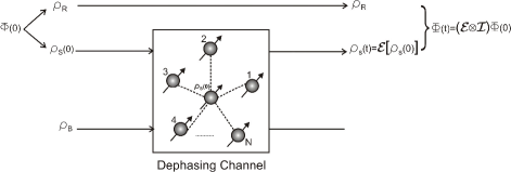
Figure 1: Communication protocol: a qubit passes through an Ising spin-star channel. This is repeated in parallel over many identical such channels.

We consider the case of an exactly solvable spin star system of $N+1$ localized spin-$\frac{1}{2}$ particles as shown in Fig. 1. The system input state $\rho_{S}(0)$ is carried by the central (system) spin. This spin interacts with $N$ noncentral spins comprising the bath. The bath spins do not interact with each other directly. The interaction between the system spin and bath is given by the Ising Hamiltonian

$$H_{I}=\alpha\sigma_{z}\otimes\sum_{n=1}^{N}g_{n}\sigma_{n}^{z},$$ (9)

where we work in $\hbar=1$ units, $g_{n}\in[-1,1]$ are dimensionless real-valued coupling constants, and $\alpha>0$ is the coupling strength having the dimension of frequency. The system and bath Hamiltonians are given by

$$H_{S} = \frac{1}{2}\omega_{0}\sigma^{z},$$ (10)

$$H_{B} = \frac{1}{2}\sum_{n=1}^{N}\Omega_{n}\sigma_{n}^{z}.$$ (11)

The frequencies $\omega_{0}$ and $\Omega_{n}$ are restricted to the interval $[-1,1]$, in frequency units. Initially, the total system is assumed to be in the product state

$$\rho(0)=\rho_{S}(0)\otimes\rho_{B},$$ (12)

with the bath in the Gibbs thermal state at inverse temperature $\beta=1/(kT)$ given by

$$\rho_{B}=\exp(-\beta H_{B})/\text{Tr}[\exp(-\beta H_{B})].$$ (13)

Since $\rho_{B}$ commutes with $H_{I}$ the bath state is stationary throughout the dynamics: $\rho_{B}(t)=\rho_{B}$. The state of the system qubit is obtained by performing a partial trace over the bath Hilbert space

$$\rho_{S}(t)=\text{Tr}_{B}\{U(t)\rho(0)U^{{\dagger}}(t))\},$$ (14)

where $U(t)=\exp[-it(H_{S}+H_{I}+H_{B})]$. The analytical solution of this model was worked out in detail in Ref. H. Krovi, O. Oreshkov, M. Ryazanov, and D. A. Lidar (2007), and we present a brief summary next.

III.2 Exact Solution

At any given time $t$, the state of the system qubit $\rho_{S}(t)$ can be written in the Kraus representation as K. Kraus (1977),

$$\rho_{S}(t)=\mathcal{E}(\rho_{S}(0))=\sum_{i,j}K_{ij}\rho_{S}(0)K_{ij}^{{\dagger}},$$ (15)

where the Kraus operators satisfy the completeness relation $\sum_{i,j}K_{ij}^{{\dagger}}K_{ij}=I_{S}$. After a transformation to the interaction picture defined by $H_{S}+H_{B}$, these operators can be expressed as

$$K_{ij}=\sqrt{\lambda_{i}}\langle j|\exp(-iH_{I}t)|i\rangle,$$ (16)

where we have introduced the spectral decomposition $\rho_{B}=\sum_{i}\lambda_{i}|i\rangle\langle i|$ of the initial bath state. For the Gibbs thermal state chosen here the eigenbasis states $\{|i\rangle\}$ are $N$-fold tensor products of the $\sigma^{z}$ eigenstates, which gives

$$\rho_{B}=\sum_{i}\frac{\exp(-\beta E_{i})}{Z}|i\rangle\langle i|,$$ (17)

where $E_{i}=\frac{1}{2}\sum_{n=1}^{N}\Omega_{n}(-1)^{i_{n}}$ is the energy of each bath eigenstate $|i\rangle$ ($i=i_{1},i_{2},\ldots,i_{N}$ is the binary expansion of the integer $i$, where $i\in[0,\ldots,2^{N}-1]$) and $Z=\sum_{i}\exp(-\beta E_{i})$ is the partition function. Therefore, the Kraus operators are

$$K_{ij}=\sqrt{\lambda_{i}}\exp(-it\alpha\widetilde{E}_{i}\sigma^{z})\delta_{ij},$$ (18)

with $\lambda_{i}=\exp(-\beta E_{i})/Z$, and $\widetilde{E}_{i}$ given by

$$\widetilde{E}_{i} = \sum_{n=1}^{N}g_{n}(-1)^{i_{n}}-\text{Tr}\{\sum_{n}g_{n}\sigma_{n}^{z}\rho_{B}\},$$ (19)

$$= \sum_{n=1}^{N}g_{n}[(-1)^{i_{n}}-\beta_{n}],$$

where $\beta_{n}=\tanh(-\frac{1}{2}\beta\Omega_{n})$. The CPTP map $\rho_{S}(0)\overset{\mathcal{E}}{\rightarrow}\rho_{S}(t)$ with the Kraus operators given by Eq. (18), represents a quantum dephasing channel, since the Kraus operators are diagonal in the reference basis $\{|0\rangle,|1\rangle\}\in\mathcal{H}_{S}$ (eigenstates of $\sigma^{z}$ with eigenvalues $\pm 1$) of the system. Moreover, as it corresponds to a non-Markovian model H. Krovi, O. Oreshkov, M. Ryazanov, and D. A. Lidar (2007), $\mathcal{E}$ represents a quantum dephasing channel with memory. We now determine the information transmission capacities of this channel.

IV Capacities of Quantum Dephasing Channel

IV.1 Classical Capacity

Dephasing channels have the characteristic property of transmitting states of a preferential orthonormal basis without introducing any error Nielsen and Chuang (2000). These basis states can be used to encode classical information, which makes these channels noiseless for the transmission of classical information D’Arrigo et al. (2007). Superpositions of the basis states will decohere, however, therefore dephasing channels are noisy for quantum information. For the dephasing channel ${\cal E}$ under consideration the preferential orthonormal basis is$\{|0\rangle,|1\rangle\}^{\otimes M}\in{\cal H}_{S}^{\otimes M}$, for $M$ parallel uses of the channel, i.e., $M$ classical bits can be transmitted noiselessly over $M$ copies of the channel.

IV.2 Quantum Capacity

Consider the communication system shown in Fig. 1. Quantum information is encoded into the system spin via a unitary transformation. The system spin is then transmitted to the receiver, over the spin-star channel. In general, one must perform the maximization of the coherent information $I_{c}$ over the $n$-fold tensor product Hilbert space ${\cal H}_{S}^{\otimes n}$. However, Devetak and Shor recently established dephasing channels as degradable channels Devetak and Shor (2005). Therefore the single channel-use formula $Q=Q_{1}$ applies, and the maximization as in Eq. (5) over the larger Hilbert space is avoided. Moreover, Arrigo et al. D’Arrigo et al. (2007) showed that for dephasing channels the coherent information $I_{c}$ is maximized by separable input states diagonalized in the reference basis. Therefore, we set the initial state of the system spin as

$$\rho_{S}(0)=\frac{1}{2}(|0\rangle\langle 0|+|1\rangle\langle 1|)=\frac{I}{2}.$$ (20)

Initially, the system spin $\rho_{S}(0)$ is coupled to a reference system $R$ such that the total system $SR$ is pure. The reference system does not undergo any dynamical evolution; it is introduced as a mathematical device to purify the initial state of the system spin. The joint initial state of the total system $SR$ is given by the maximally entangled state

$$|\Phi\rangle=\frac{1}{\sqrt{2}}(|00\rangle+|11\rangle).$$ (21)

Dephasing channels are unital channels, i.e., $\mathcal{E}(I)=I$, therefore the state of system spin is unaltered after interacting with the Ising bath

$$\rho_{S}(t)=\rho_{S}(0)=\frac{I}{2}.$$ (22)

However, the total system $SR$ decoheres as a result of the interaction and is mapped to a mixed state, whose diagonal elements (“populations”) are unaffected, but whose off-diagonal elements (“coherences”) are:

$$\rho_{SR}(t) = (\mathcal{E}\otimes\mathcal{I})(|\Phi\rangle\langle\Phi|)$$ (23)

$$= \sum_{i,j}(K_{ij}\otimes I)(|\Phi\rangle\langle\Phi|)(K_{ij}^{{\dagger}}\otimes I),$$

$$= \frac{1}{2}(|00\rangle\langle 00|+|11\rangle\langle 11|)$$

$$+\frac{1}{2}\sum_{i}\lambda_{i}(e^{-2i\alpha t\widetilde{E}_{i}}|00\rangle\langle 11|$$

$$+e^{+2i\alpha t\widetilde{E}_{i}}|11\rangle\langle 00|).$$

The quantum capacity $Q$ of the dephasing channel is now obtained by using Eq. (5), making use of the single channel-use formula $Q=Q_{1}$ and the fact that the coherent information is maximized by our chosen initial state $\rho_{S}(0)$:

$$Q = Q_{1}=\max_{\rho_{S}\in\mathcal{H}_{S}}S[\mathcal{E}(\rho_{S})]-S[(\mathcal{E}\otimes\mathcal{I})(|\Phi\rangle\langle\Phi|)]$$ (24)

$$= S[\mathcal{E}(I/2)]$$

$$-S[(\mathcal{E}\otimes\mathcal{I})(\frac{1}{\sqrt{2}}(|00\rangle+|11\rangle)\frac{1}{\sqrt{2}}(\langle 00|+\langle 11|))]$$

$$= S[I/2]-S[\rho_{SR}(t)].$$

This yields:

$$Q(t)=1+\sum_{k=1}^{4}{\large\chi}_{k}\log_{2}{\large\chi}_{k},$$ (25)

where ${\large\chi}_{1}={\large\chi}_{2}=0$ and

$${\large\chi}_{3}=\frac{1}{2}[1+\frac{1}{Z}|\Pi_{N}|],\quad{\large\chi}_{4}=\frac{1}{2}[1-\frac{1}{Z}|\Pi_{N}|],$$

are the eigenvalues of the state $\rho_{SR}(t)$, and where

$$\Pi_{N}(t)=\sum_{i=0}^{2^{N}-1}e^{-\sum_{n=1}^{N}(\frac{1}{2}\beta\Omega_{n}+2i\alpha tg_{n})(-1)^{i_{n}}}.$$ (26)

Next we calculate the entanglement-assisted capacities of the dephasing channel.

IV.3 Entanglement-Assisted Capacities

The communication protocol of entanglement-assisted capacities can also be described using Fig. 1. Prior to the communication the sender and receiver share a maximally entangled state given by Eq. (21). The first qubit of the entangled pair belongs to the sender: $\rho_{S}(0)={\rm Tr}_{R}(|\Phi\rangle\langle\Phi|)=I/2$, and interacts with the bath. Unlike the quantum capacity protocol, the second qubit is not a mathematical device and corresponds to the qubit in possession of the receiver prior to the communication. Therefore, it is again considered to have been transmitted over the identity channel.

Now note that in our case, since $S(\rho_{S})=1$ and $Q=Q_{1}$, it follows from Eqs. (5) and (7) that the quantum capacity is related to the entanglement-assisted classical capacity via the simple formula

$$C_{E}=1+Q=2+\sum_{i=1}^{4}{\large\chi}_{i}\log_{2}{\large\chi}_{i},$$ (27)

while the entanglement-assisted quantum capacity is

$$Q_{E}=\frac{C_{E}}{2}=1+\frac{1}{2}\sum_{i=1}^{4}{\large\chi}_{i}\log_{2}{\large\chi}_{i}.$$ (28)

Next, we are interested in the classical capacity assisted by limited entanglement. Consider the situation when instead of a maximally entangled state, an ensemble of orthogonal states

$$|\Phi_{1}\rangle = \cos\theta|00\rangle+\sin\theta|11\rangle,$$

$$|\Phi_{2}\rangle = \sin\theta|00\rangle-\cos\theta|11\rangle,$$

$$|\Phi_{3}\rangle = \cos\theta|01\rangle+\sin\theta|10\rangle,$$

$$|\Phi_{4}\rangle = \sin\theta|01\rangle-\cos\theta|10\rangle,$$ (29)

is shared prior to the communication, where $0\leq\theta\leq\frac{\pi}{4}$. As above the first and second qubits belong to the sender and receiver, respectively. We show in Appendix A that the classical capacity assisted by limited entanglement [Eq. (8)] is attained when all states $\{|\Phi_{i}\rangle\}_{i=1}^{4}$ are equiprobable, and that this yields:

$$C_{E}^{\lim} = -[\cos^{2}\theta\log_{2}\cos^{2}\theta+\sin^{2}\theta\log_{2}\sin^{2}\theta]+1$$ (30)

$$+\sum_{i=1}^{4}\omega_{i}\log_{2}\omega_{i},$$

with $\omega_{1}=\omega_{2}=0$ and

$$\omega_{3} = \frac{1}{2}[1+\{(\frac{2\cos\theta\sin\theta}{Z}|\Pi_{N}|)^{2}+\cos^{2}2\theta\}^{\frac{1}{2}}],$$

$$\omega_{4} = \frac{1}{2}[1-\{(\frac{2\cos\theta\sin\theta}{Z}|\Pi_{N}|)^{2}+\cos^{2}2\theta\}^{\frac{1}{2}}].$$ (31)

For $\theta=0$ the states given by Eq. (29) are product states and we recover the classical capacity which is equal to one. The capacity $C_{E}^{\lim}$ increases as we increase the value of $\theta$, attaining its maximum for $\theta=\frac{\pi}{4}$ for which the states are maximally entangled and Eq. (30) reduces to Eq. (27).

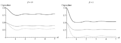
Figure 2: Capacities $C_{E}=1+Q$ (solid, thick), $Q_{E}=C_{E}/2$ (solid, thin) and $Q$ (dashed) of qubit coupled to an Ising spin bath with $N=4$, for random values of $g_{n}$ and $\Omega_{n}$. Left: $\beta=10$, right: $\beta=1$. See text for details.

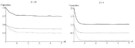
Figure 3: Same as Fig. 2, with $N=100$.

Plots of capacities for random values of couplings $g_{n}$ and bath frequencies $\Omega_{n}$, are given in Figs. 2 and 3. We generate real, random values of $g_{n}$ and $\Omega_{n}$ uniformly distributed in the interval $[-1,1]$ and plot average capacities for $50$ random ensembles. In Fig. 2, we plot the capacities of the system spin coupled to a bath with $N=4$ spins. We plot the capacities at low and high temperatures in order to study the effect of bath temperature. For low temperature ($\beta=10$), the bath is not too noisy and the system spin retains its coherence well. The capacities do not acquire their minimum values and partial recurrences occur, with an amplitude that diminishes over time. At high temperature ($\beta=1$) the capacities rapidly decrease to their minimum values and the recurrences are of smaller amplitude. As the system spin loses its coherence to the Ising bath, the entanglement shared between the sender and receiver is destroyed and $C_{E}$ is reduced to its minimum value of one. This corresponds to the qubit in possession of the receiver prior to the communication. The quantum capacity $Q$, which is a measure of the coherent information transmitted, is reduced to zero as the system spin decoheres completely. As we increase the number of bath spins to $N=100$, we observe a similar dependence on bath temperature. The main difference compared to the case of a small number of bath spins is the drastically diminished amplitude of the recurrences. As noted in Ref. H. Krovi, O. Oreshkov, M. Ryazanov, and D. A. Lidar (2007), this behavior is due to the averaging of the positive and negative oscillations which arise for different values of the parameters $g_{n}$ and $\Omega_{n}$.

IV.4 Limiting Cases

IV.4.1 Equal Couplings and Frequencies

If the bath spins have equal frequencies $\Omega_{n}\equiv\Omega$ $\forall n$, and couplings $g_{n}\equiv g$ $\forall n$ with the system spin then Eq. (26) reduces to

$$\Pi_{N} = \sum_{i=0}^{2^{N}-1}e^{-f(t)\sum_{n=1}^{N}(-1)^{i_{n}}}$$ (32)

$$= \sum_{k=0}^{N}\binom{N}{k}e^{(2k-N)f(t)}=(2\cosh[f(t)])^{N},$$

where

$$f(t)=\frac{1}{2}\beta\Omega+2i\alpha tg.$$ (33)

The second equality in Eq. (32) follows from the fact that the term $\sum_{n=1}^{N}(-1)^{i_{n}}=N-2k$ for $i$ with Hamming weight $k$, of which there are $\binom{N}{k}$ cases for $i\in[0,\ldots,2^{N}-1]$. Therefore $|\Pi_{N}|=2^{N}\sqrt{(\cos^{2}(2\alpha tg)\cosh^{2}(\frac{\beta}{2}\Omega)+\sin^{2}(2\alpha tg)\sinh^{2}(\frac{\beta}{2}\Omega))^{N}}$ is periodic with period $T_{p}=\pi/(2\alpha g)$, and the same is true of all the capacities computed above. At these times the bath spins destructively interfere and the dephasing channel becomes noiseless for information transmission. In the high temperature limit $\beta\Omega\rightarrow 0$, and $|\Pi_{N}|\rightarrow(2\cos(2\alpha tg))^{N}$, so that the capacities exhibit full periodic recurrences independently of $N$, in contrast to the results for random couplings and frequencies. Clearly, as $N$ gets larger, these recurrences become sharper, until in the limit $N\rightarrow\infty$ they become isolated peaks, as shown in the right-side panels of Figs. 4 and 5. In the low temperature limit $\beta\Omega\rightarrow\infty$ and $|\Pi_{N}|\rightarrow\exp(\frac{N}{2}\beta\Omega)$, but so does the partition function $Z=\sum_{i=0}^{2^{N}-1}e^{-\frac{1}{2}\beta\Omega\sum_{n=1}^{N}(-1)^{i_{n}}}=(2\cosh[f(0)])^{N}\rightarrow\exp(\frac{N}{2}\beta\Omega)$, so that ${\large\chi}_{3},{\large\chi}_{4}\rightarrow 1$, and all the capacities are saturated at their maximum values. For small, but finite temperatures, the capacities exhibit oscillations with an amplitude that grows with $N$, as can be seen in the left-side panels of Figs. 4 and 5. This is in contrast to the case of random couplings seen in Figs. 2 and 3; there destructive interference caused a cancellation of these oscillations, while in the case of equal couplings the capacity oscillations survive and grow with the number of bath spins, reflecting the increased information transfer from the system to the bath as a function of bath size.

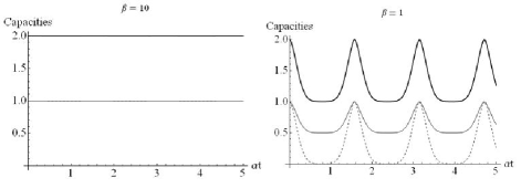
Figure 4: Capacities $C_{E}$ (solid, thick), $Q_{E}$ (solid, thin) and $Q$ (dashed) of a qubit coupled to an Ising spin bath with $N=4$, for $g_{n}=1$ and $\Omega_{n}=1$ $\forall n$. Left: $\beta=10$, right: $\beta=1$.

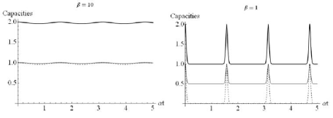
Figure 5: Same as Fig. 4, with $N=100$.

IV.4.2 Large $N$

Without symmetries in the coupling constants or frequencies the capacities rapidly decrease to their minimum values and we find no recurrences for $N\gg 1$, high temperature and uniformly distributed random values of $g_{n}$ and $\Omega_{n}$. However, partial recurrences occur in this situation for small temperature.

IV.4.3 Short Times

The capacities are flat initially and do not decay exponentially in the limit of short times $\alpha t\ll 1$, provided that the temperature and number of bath spins $N$ is not too large. This is somewhat similar to the Zeno behavior pointed out in Ref. H. Krovi, O. Oreshkov, M. Ryazanov, and D. A. Lidar (2007).

V Summary and Conclusions

We have studied an exactly solvable spin-star system for transmission of classical and quantum information. The information is encoded into a system spin which interacts with a spin-bath via arbitrary Ising couplings. We considered the “parallel uses” setting of a memoryless quantum channel, where multiple copies of the system spin are transmitted simultaneously via the same number of copies of the spin bath. As our model is described by the dephasing channel, classical information can be transmitted noiselessly, while the quantum capacity can be determined via the “single-letter” formula $Q=Q_{1}$, i.e., it suffices to consider a single copy of the spin-star system. We analytically determined the quantum capacities of this communication system, which exhibit a strong dependence on the couplings of the bath spins with the system, and on the bath temperature. The Ising spin bath becomes noisier as the temperature is increased, and the capacities rapidly deteriorate. For random couplings and frequencies, recurrences are of small amplitude and die out rapidly. However, for equal couplings and frequencies full periodic recurrences occur independently of the number of bath spins. These recurrences are a signature of the non-Markovian nature of the spin-bath. At low temperature the quantum capacities remain high when the number of bath spins is not too large.

Appendix A Derivation of the result for the classical capacity assisted by limited entanglement

We prove Eq. (30). Without loss of generality the ensemble of orthogonal states given by Eq. (29) can be assumed to appear with probabilities parametrized as

$$p_{1}(x_{1},x_{2}) = \cos^{2}x_{1}\cos^{2}x_{2},$$

$$p_{2}(x_{1},x_{2}) = \sin^{2}x_{1}\cos^{2}x_{2},$$

$$p_{3}(x_{1},x_{2}) = \cos^{2}x_{1}\sin^{2}x_{2},$$

$$p_{4}(x_{1},x_{2}) = \sin^{2}x_{1}\sin^{2}x_{2},$$ (34)

where $0\leq\theta,x_{1},x_{2}\leq\frac{\pi}{4}$. We will show by explicit calculation that for our pure dephasing model only the second term in Eq. (8) for the classical capacity assisted by limited entanglement depends on the parameters $x_{1},x_{2}$. Hence the maximization can be carried out, for fixed $\theta$, by maximizing only this second term.

The states input to the quantum dephasing channel obtained from Eq. (29) are

$$\rho_{S,1} = \text{Tr}_{R}(|\Phi_{1}\rangle\langle\Phi_{1}|)=\cos^{2}\theta|0\rangle\langle 0|+\sin^{2}\theta|1\rangle\langle 1|,$$

$$\rho_{S,2} = \text{Tr}_{R}(|\Phi_{2}\rangle\langle\Phi_{2}|)=\sin^{2}\theta|0\rangle\langle 0|+\cos^{2}\theta|1\rangle\langle 1|,$$

$$\rho_{S,3} = \text{Tr}_{R}(|\Phi_{3}\rangle\langle\Phi_{3}|)=\cos^{2}\theta|0\rangle\langle 0|+\sin^{2}\theta|1\rangle\langle 1|,$$

$$\rho_{S,4} = \text{Tr}_{R}(|\Phi_{4}\rangle\langle\Phi_{4}|)=\sin^{2}\theta|0\rangle\langle 0|+\cos^{2}\theta|1\rangle\langle 1|,$$

therefore, for all $\rho_{S,i}$

$$S(\rho_{S,i})=-[\cos^{2}\theta\log_{2}\cos^{2}\theta+\sin^{2}\theta\log_{2}\sin^{2}\theta].$$ (36)

This results in the following expression for the first term in Eq. (8):

$$\sum_{i}p_{i}(x_{1},x_{2})S(\rho_{S,i})$$

$$=-(\cos^{2}x_{1}\cos^{2}x_{2}+\sin^{2}x_{1}\cos^{2}x_{2}$$

$$\quad+\cos^{2}x_{1}\sin^{2}x_{2}+\sin^{2}x_{1}\sin^{2}x_{2})$$

$$\quad\times[\cos^{2}\theta\log_{2}\cos^{2}\theta+\sin^{2}\theta\log_{2}\sin^{2}\theta],$$

$$=-[\cos^{2}\theta\log_{2}\cos^{2}\theta+\sin^{2}\theta\log_{2}\sin^{2}\theta],$$ (37)

where we have used the normalization $\sum_{i=1}^{4}p_{i}(x_{1},x_{2})=1,\forall x_{1},x_{2}$. This yields the first term in Eq. (30).

Next we calculate the second term in Eq. (8). The output state is

$$\mathcal{E}(\sum_{i}p_{i}(x_{1},x_{2})\rho_{S,i})$$

$$=\sum_{i,j}K_{ij}(\sum_{i}p_{i}(x_{1},x_{2})\rho_{S,i})K_{ij}^{{\dagger}},$$ (38)

where

$$\sum_{i}p_{i}(x_{1},x_{2})\rho_{S,i}$$

$$=[\cos^{2}\theta(\cos^{2}x_{1}\cos^{2}x_{2}+\cos^{2}x_{1}\sin^{2}x_{2})$$

$$\quad+\sin^{2}\theta(\sin^{2}x_{1}\sin^{2}x_{2}+\sin^{2}x_{1}\cos^{2}x_{2})]|0\rangle\langle 0|$$

$$\quad+[\cos^{2}\theta(\sin^{2}x_{1}\sin^{2}x_{2}+\sin^{2}x_{1}\cos^{2}x_{2})$$

$$\quad+\sin^{2}\theta(\cos^{2}x_{1}\cos^{2}x_{2}+\cos^{2}x_{1}\sin^{2}x_{2})]|1\rangle\langle 1|$$

$$=(\cos^{2}\theta\cos^{2}x_{1}+\sin^{2}\theta\sin^{2}x_{1})|0\rangle\langle 0|$$

$$\quad+(\cos^{2}\theta\sin^{2}x_{1}+\sin^{2}\theta\cos^{2}x_{1})|1\rangle\langle 1|.$$ (39)

Since this state is diagonal (“classical”) it is invariant under the dephasing channel with Kraus operators given by Eq. (18). Therefore the eigenvalues of the output state (38) are

$$\upsilon_{1} = \cos^{2}\theta\cos^{2}x_{1}+\sin^{2}\theta\sin^{2}x_{1},$$

$$\upsilon_{2} = \cos^{2}\theta\sin^{2}x_{1}+\sin^{2}\theta\cos^{2}x_{1},$$ (40)

and

$$S[\mathcal{E}(\sum_{i}p_{i}(x_{1},x_{2})\rho_{S,i})]=-\sum_{i=1}^{2}\upsilon_{i}\log_{2}\upsilon_{i}.$$ (41)

Finally, we calculate the third term in Eq. (8):

$$(\mathcal{E}\otimes I)(|\Phi_{i}\rangle\langle\Phi_{i}|)$$

$$=\sum_{i,j}(K_{ij}\otimes I)(|\Phi_{i}\rangle\langle\Phi_{i}|)(K_{ij}^{{\dagger}}\otimes I),$$ (42)

which for all $|\Phi_{i}\rangle$ has eigenvalues $\omega_{1}=\omega_{2}=0$ and $\omega_{3},\omega_{4}$ are given in Eq. (31). The third term in Eq. (8) is thus

$$\sum_{i}p_{i}(x_{1},x_{2})S[(\mathcal{E}\otimes I)(|\Phi_{i}\rangle\langle\Phi_{i}|)]$$

$$=-\sum_{i=1}^{4}\omega_{i}\log_{2}\omega_{i},$$ (43)

where, as for Eq. (37), we have used the normalization $\sum_{i=1}^{4}p_{i}=1$. This yields the third term in Eq. (30).

Thus, indeed only the second term in Eq. (8) depends on $x_{1},x_{2}$, and for a given value of $\theta$, the classical capacity assisted by limited entanglement is maximized by maximizing Eq. (41). The maximum is attained when the output state (38) is fully mixed, i.e., when its eigenvalues $\upsilon_{1}=\upsilon_{2}=1/2$. This occurs when $x_{1}=x_{2}=\frac{\pi}{4}$, i.e., when we have an equiprobable ensemble of the states. This gives rise to the $1$ in Eq. (30).

References

- Bennett and Shor (1998) C. Bennett and P. Shor, IEEE Trans. Inf. Theory 44, 2724 (1998).
- Nielsen and Chuang (2000) M. Nielsen and I. Chuang, Quantum Computation and Quantum Information (Cambridge University Press, Cambridge, England, 2000).
- Cover and Thomas (1991) T. M. Cover and J. A. Thomas, Elements of Information Theory (Wiley, New York, 1991).
- Shannon (1948) C. Shannon, Bell Sys. Tech. J. 27, 379 (1948).
- Bennett and Shor (2004) C. H. Bennett and P. W. Shor, Science 303, 1784 (2004).
- Hausladen et al. (1996) P. Hausladen, R. Jozsa, B. Schumacher, M. Westmoreland, and W. K. Wootters, Phys. Rev. A 54, 1869 (1996).
- Schumacher and Westmoreland (1997) B. Schumacher and M. D. Westmoreland, Phys. Rev. A 56, 131 (1997).
- Lloyd (1997) S. Lloyd, Phys. Rev. A 55, 1613 (1997).
- Bennett et al. (1997) C. H. Bennett, D. P. DiVincenzo, and J. A. Smolin, Phys. Rev. Lett. 78, 3217 (1997).
- Adami and Cerf (1997) C. Adami and N. J. Cerf, Phys. Rev. A 56, 3470 (1997).
- Barnum et al. (1998) H. Barnum, M. A. Nielsen, and B. Schumacher, Phys. Rev. A 57, 4153 (1998).
- Bennett et al. (1999) C. H. Bennett, P. W. Shor, J. A. Smolin, and A. V. Thapliyal, Phys. Rev. Lett. 83, 3081 (1999).
- Bennett et al. (2002) C. Bennett, P. Shor, J. Smolin, and A. Thapliyal, IEEE Trans. Inf. Theory 48, 2637 (2002).
- Shor (2002) P. Shor, The quantum channel capacity and coherent information, Tech. Rep., Lecture Notes MSRI Workshop on quantum computation (2002), URL http://www.msri.org/publications/ln/msri/2002/quantumcrypto/s%hor/1/.
- Holevo (2002) A. S. Holevo, J. Math. Phys. 43, 4326 (2002).
- Liang (2002) X. T. Liang, Mod. Phys. Lett. 16, 19 (2002).
- Daffer et al. (2003) S. Daffer, K. Wódkiewicz, and J. K. McIver, Phys. Rev. A 67, 062312 (2003).
- Shor (2004a) P. W. Shor, Quantum Inf. Comput. 4, 537 (2004a).
- Kretschmann and Werner (2004) D. Kretschmann and R. F. Werner, New J. Phys. 6, 26 (2004).
- Devetak (2005) I. Devetak, IEEE Trans. Inf. Theory 51, 44 (2005).
- Giovannetti and Fazio (2005) V. Giovannetti and R. Fazio, Phys. Rev. A 71, 032314 (2005).
- Wolf and Pérez-García (2007) M. M. Wolf and D. Pérez-García, Phys. Rev. A 75, 012303 (2007).
- Macchiavello and Palma (2002) C. Macchiavello and G. M. Palma, Phys. Rev. A 65, 050301 (2002).
- Yeo and Skeen (2003) Y. Yeo and A. Skeen, Phys. Rev. A 67, 064301 (2003).
- Macchiavello et al. (2004) C. Macchiavello, G. M. Palma, and S. Virmani, Phys. Rev. A 69, 010303 (2004).
- Bowen and Mancini (2004) G. Bowen and S. Mancini, Phys. Rev. A 69, 012306 (2004).
- Arshed and Toor (2006) N. Arshed and A. H. Toor, Phys. Rev. A 73, 014304 (2006).
- D’Arrigo et al. (2007) A. D’Arrigo, G. Benenti, and G. Falci, New J. Phys. 9, 310 (2007).
- Plenio and Virmani (2007) M. B. Plenio and S. Virmani, Phys. Rev. Lett. 99, 120504 (2007).
- Bayat et al. (2008) A. Bayat, D. Burgarth, S. Mancini, and S. Bose, Phys. Rev. A 77, 050306 (2008).
- H.-P. Breuer and F. Petruccione (2002) H.-P. Breuer and F. Petruccione, The Theory of Open Quantum Systems (Oxford University Press, Oxford, 2002).
- Breuer et al. (2009) H.-P. Breuer, E.-M. Laine, and J. Piilo, Phys. Rev. Lett. 103, 210401 (2009).
- Carmichael (1993) H. Carmichael, An open systems approach to quantum optics, no. m18 in Lecture notes in physics (Springer-Verlag, Berlin, 1993).
- Slichter (1996) C. Slichter, Principles of Magnetic Resonance, no. 1 in Springer Series in Solid-State Sciences (Springer, Berlin, 1996).
- R. Alicki, D. A. Lidar, and P. Zanardi (2006) R. Alicki, D. A. Lidar, and P. Zanardi, Phys. Rev. A 73, 052311 (2006).
- U. Weiss (1993) U. Weiss, Quantum Dissipative Systems (World Scientific, Singapore, 1993).
- A. Shabani and D. A. Lidar (2005) A. Shabani and D. A. Lidar, Phys. Rev. A 71, 020101(R) (2005).
- H. Krovi, O. Oreshkov, M. Ryazanov, and D. A. Lidar (2007) H. Krovi, O. Oreshkov, M. Ryazanov, and D. A. Lidar, Phys. Rev. A 76, 052117 (2007).
- Loss and DiVincenzo (1998) D. Loss and D. DiVincenzo, Phys. Rev. A 57, 120 (1998).
- B. E. Kane (1998) B. E. Kane, Nature 393, 133 (1998).
- Vrijen et al. (2000) R. Vrijen, E. Yablonovitch, H. J. K. Wang, A. Balandin, V. Roychowdhury, T. Mor, and D. DiVincenzo, Phys. Rev. A 62, 012306 (2000).
- Petta et al. (2005) J. Petta, A. Johnson, J. Taylor, E. Laird, A. Yacoby, M. D. Lukin, C. Marcus, M. Hanson, and A. C. Gossard, Science 309, 2180 (2005).
- Morton et al. (2008) J. J. L. Morton, A. M. Tyryshkin, R. M. Brown, S. Shankar, B. W. Lovett, A. Ardavan, T. Schenkel, E. E. Haller, J. W. Ager, and S. A. Lyon, Nature 455, 1085 (2008).
- Bose (2007) S. Bose, Contemp. Phys 48, 13 (2007).
- Hutton and Bose (2004) A. Hutton and S. Bose, Phys. Rev. A 69, 042312 (2004).
- Yuan et al. (2007) X.-Z. Yuan, H.-S. Goan, and K.-D. Zhu, Phys. Rev. B 75, 045331 (2007).
- Breuer et al. (2004) H.-P. Breuer, D. Burgarth, and F. Petruccione, Phys. Rev. B 70, 045323 (2004).
- Hamdouni et al. (2006) Y. Hamdouni, M. Fannes, and F. Petruccione, Phys. Rev. B 73, 245323 (2006).
- A. Shabani and D. A. Lidar (2009) A. Shabani and D. A. Lidar, Phys. Rev. Lett. 102, 100402 (2009).
- King et al. (2007) C. King, K. Matsumoto, M. Nathanson, and M. B. Ruskai, Markov Process and Related Fields 13, 391 (2007).
- Devetak and Shor (2005) I. Devetak and P. W. Shor, Commun. Math. Phys. 256, 287 (2005).
- Holevo (1973) A. S. Holevo, Probl. Inf. Transm. 9, 177 (1973).
- Hastings (2009) M. B. Hastings, Nature Phys. 5, 255 (2009).
- Shor (2004b) P. W. Shor, Commun. Math. Phys. 246, 453 (2004b).
- T.A. Brun, I. Devetak, M.-H. Hsieh (2006) T.A. Brun, I. Devetak, M.-H. Hsieh, Science 314, 436 (2006).
- Bennett and Wiesner (1992) C. Bennett and S. Wiesner, Phys. Rev. Lett. 69, 2881 (1992).
- C.H. Bennett, G. Brassard, C. Crépeau, R. Jozsa, A. Peres and W.K. Wootters (1993) C.H. Bennett, G. Brassard, C. Crépeau, R. Jozsa, A. Peres and W.K. Wootters, Phys. Rev. Lett. 70, 1895 (1993).
- K. Kraus (1977) K. Kraus, Ann. of Phys. 64, 311 (1977).