2006
\degreesemester
\degreeDoctor of Philosophy
\chairProfessor Ignatius Arrogant
\othermembersProfessor Ivory Insular
Professor General Reference
\numberofmembers3
\fieldAboriginal Basketry
\campusBerkeley
Nonlinear Processes in Coronal Heating and Slow Solar Wind Acceleration
“…highly nonlinear problems of magnetohydrodynamics…are too difficult for exact analytical treatment and must be left to the mastication of computer wallahs.”
Donald Lynden-Bell, Mon. Not. R. Astron. Soc. 267, 146 (1994)
Acknowledgements.
This work has been supported in part by a fellowship of the Università degli Studi di Pisa. I am grateful to the many people who helped me throughout this work. Many thanks to my official and unofficial supervisors, Russell Dahlburg, Giorgio Einaudi, Steve Shore and Marco Velli. In particular I would like to thank Russ Dahlburg, who made possible a one year visit at Naval Research Laboratory. I would also like to thank the IPAM program “Grand Challenge Problems in Computational Astrophysics” at UCLA, where part of this work has been performed. The 3D visualization of the numerical simulations has been made easy (and possible) thanks to Viggo Hansteen, who has introduce me to OpenDX, a user-friendly program with which all the 3D figures and movies have been done. I would also like to thank Francesco Malara for the many stimulating and useful discussions we have had while I was writing the manuscript, and Zoran Mikic, Jon Linker and Roberto Lionello for their suggestions. Finally, I would like to thank the referees who have carefully read the manuscript: Claudio Chiuderi, Francesco Pegoraro and Dalton Schnack. I would also like to thank my friends and colleagues who have made less painful my stay in Pisa, in particular Andrea Dotti, Daniele Ippolito, Gianluca Lamanna and, last but not least, my cousin Massimo Romano who has patiently and repeatedly given me hospitality during the last few years.Part I Coronal Heating
Chapter 0 The Coronal Heating Problem
The Sun, our nearest star, is both the source of energy for life on Earth and a unique physics laboratory. Energy produced in the core of the Sun is transported to its surface and atmosphere. From here, through radiation and a flow of particles (the solar wind), it affects the Earth and forms the so-called heliosphere, a cavity inside the local interstellar medium which extends beyond the solar system boundaries.
The visible surface of the Sun, the photosphere, has a temperature of about and emits mostly visible light. High energy radiation (EUV, FUV, up to X-rays) is produced in the upper layers of the atmosphere: the chromosphere, the transition region and the Corona. On the other hand the steady production of this kind of radiation requires high temperatures, and the highest temperatures are localized in the Corona. Hence this gives rise to the so-called Coronal heating problem: Corona is counterintuitively much hotter (millions of degrees ) than the underlying photosphere. While there is general agreement that the magnetic field plays a fundamental role, and that the source of this energy derives from convective motions in the photosphere (which have more than enough energy), the debate currently focuses on what physical mechanisms can transfer, store, and dissipate this energy between the photosphere and the corona.
1 The Sun: its Interior and Atmosphere
The solar interior is conveniently separated into zones by the different physical processes at work. The pressure, density, and temperature decrease going outward, from the center up to the surface, located at 1 solar radius (). Energy is generated by nuclear reactions in the core, the innermost 25% of the radius. This energy is transported outward by radiation through the radiative zone and by convective flows through the convection region, the outermost 30%.
The convection zone is the outermost layer of the solar interior. It extends from a depth of about up to the visible surface. At the base of the convection zone the temperature is about . This temperature is low enough that the heavier ions are not totally ionized. This increases the cross section for the radiation, ultimately trapping more heat, which in turns makes the plasma unstable to convection. Convection occurs when the temperature gradient required to radiatively transport the energy is larger than the adiabatic gradient, i.e. the rate at which the temperature would fall if a volume of material expanded adiabatically while rising toward the surface. Where this occurs a parcel of plasma displaced upward will be warmer than its surroundings and will continue to rise, i.e. convection instability sets in. Convective motions are quite efficient in carrying heat to the solar surface, and while the plasma rises it expands and cools. At the visible surface the temperature drops to and the density to .
The photosphere is the visible surface of the Sun. Since the Sun is made of ionized gas, this surface is not sharply defined, and it is actually a layer about thick (very thin compared to the radius of the Sun). A number of features, which are relevant for coronal heating models, are observed in the photosphere, including the dark sunspots, the bright faculae, and granules.

Sunspots (Fig. 1) appear as comparatively isolated dark regions on the surface. They typically last for several days, although very large ones may live for several weeks. Sunspots are magnetic regions on the Sun characterized by a magnetic field of the order of about gauss, noticeably stronger that the surrounding field (a few gauss). Sunspots usually come in groups with pairs of spots, with opposite field polarity. The field is strongest in the umbra, the darkest part of the sunspots, while it is weaker and more horizontal in the penumbra, the brighter part surrounding the umbra. Temperatures in the dark centers of sunspots drop to about , compared to for the surrounding photosphere, due to the presence of the strong magnetic field which partially inhibits convective motions.
Faculae are bright areas that are most easily seen near the limb, or edge, of the solar disk. These are also magnetic regions but the field is concentrated in much smaller bundles than in sunspots. While the sunspots tend to make the Sun look darker, the faculae make it look brighter. During a sunspot cycle the faculae actually win out over the sunspots and make the Sun appear slightly (about 0.1%) brighter at sunspot maximum that at sunspot minimum.
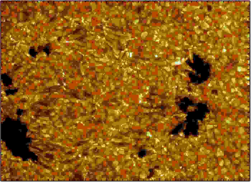
Granules (Fig. 2 and also Fig. 1) are small (their typical size is about ) cellular features that cover the entire Sun except for those areas covered by sunspots. These are the tops of convection cells where hot plasma rises up from the interior in the bright areas, spreads out across the surface, cools and then sinks inward along the dark lanes. Individual granules last for only about 8 minutes. The granulation pattern is continually changing as old granules are pushed aside by newly emerging ones (see movie from the Swedish 1-meter Solar Telescope). The average speed of the flow within the granules is , but it can reach supersonic speeds of more than . This flow, and its interaction with the magnetic field, generate waves which then propagates toward the upper layers of the atmosphere.
Supergranules are another flow pattern present in the photosphere, at a larger scale (about across) than granules. These features also cover the entire Sun and are continually evolving. Individual supergranules last for a day or two and have flow speeds of about .
The chromosphere is an irregular layer, thick, above the photosphere where the temperature rises from (the temperature minimum) at its base to about at the top. At these higher temperatures hydrogen emits light that gives off a reddish color (H emission). This colorful (chromo = color) emission can be seen in prominences that project above the limb of the sun during total solar eclipses. The chromosphere is the site of activity as well. Solar flares, prominence and filament eruptions, and the flow of material in post-flare loops can all be observed over the course of just a few minutes.
The transition region is a thin and very irregular layer of the Sun’s atmosphere that separates the chromosphere from the much hotter corona. The temperature changes rapidly from up to over a distance. Hydrogen is ionized at these temperatures and is therefore difficult to detect. Instead the light emitted by the transition region is dominated by such ions as C IV, O IV, and Si IV that emit light in the far ultraviolet region ( Å) of the solar spectrum that is only accessible from space.
2 The Solar Corona
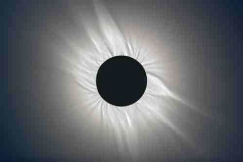
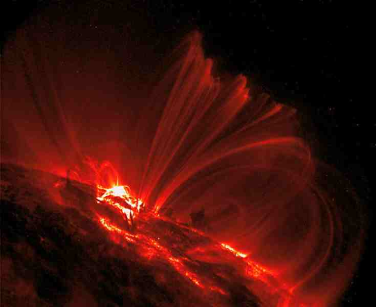
The Corona is the Sun’s outer atmosphere. Most of the visible light coming from the corona is light coming from the photosphere diffused trough Thompson scattering. This results in a faint emission compared to the photosphere, and it only becomes visible during total eclipses of the Sun, as shown in Fig. 3, or using a special instrument called coronagraph. The corona displays a variety of features including streamers, plumes, and loops. These features change from eclipse to eclipse and the overall shape of the corona changes with the sunspot cycle. However, during the few fleeting minutes of totality few, if any, changes are seen in these coronal features.
Early observations by Harkness and Young in 1869 of the visible spectrum of the corona revealed bright emission lines at wavelengths that did not correspond to any known materials. This led astronomers to propose the existence of “coronium” as the principal gas in the corona. The true nature of the corona remained a mystery until 1939, when Grotrian and Edlen identified the Fe XIV and Ni XVI lines in the corona. The corona is in fact heated to temperatures greater than . At these high temperatures both hydrogen and helium (the two dominant elements), and even minor elements like carbon, nitrogen, and oxygen are totally ionized. Only the heavier trace elements like iron and calcium are able to retain a few of their electrons. It is emission from these highly ionized elements that produces the spectral emission lines that were so mysterious to early astronomers.
The corona shines brightly in x-rays because of its high temperature. On the other hand, the cooler solar photosphere emits very few x-rays. This allows us to view the corona across the disk of the Sun when we observe the Sun in X-rays. To do this we must first design optics that can image x-rays and then we must get above the Earth’s atmosphere, which shields the Earth from this high energy radiations. In the early 1970s Skylab carried an x-ray telescope that revealed coronal holes and coronal bright points for the first time (these features were actually visible in earlier sounding rocket data, but they were not recognized). In the 1990s Yohkoh provided a wealth of information and images on the solar corona. Today SOHO and TRACE satellites are obtaining new and exciting observations of the Sun’s corona, its features, and its dynamic character.
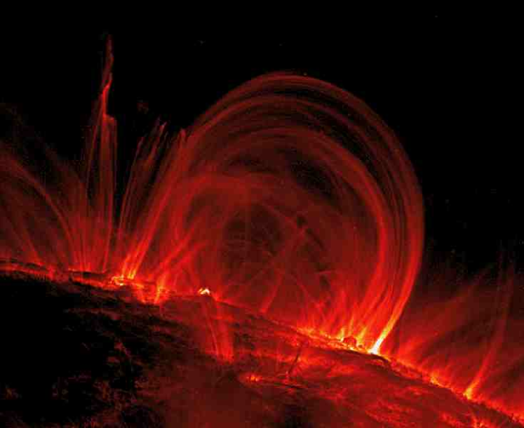
Coronal loops are found above sunspots and active regions. These structures are associated with the closed field lines that connect magnetic regions on the solar surface. Many coronal loops last for days or weeks but most change quite rapidly.
Coronal holes, where the corona is dark, were discovered when X-ray telescopes were first flown above the earth’s atmosphere to reveal the structure of the corona across the solar disc. They are associated with “open” magnetic field lines and are often found at the Sun’s poles (a region that is currently studied by the Ulysses mission). The high-speed solar wind is known to originate in coronal holes.
Different layers of the solar atmosphere are characterized by different features, but most of these features are connected one another by the magnetic field. At solar minimum the solar magnetic field is approximately a dipole field, with the magnetic axis aligned to the rotational axis, so that we have “open” magnetic field around polar regions and closed magnetic structures around the equator. This picture is, of course, an approximation and the major departures are at the large scales the presence of an heliospheric current sheet (a region where the magnetic field changes rapidly its polarity), and at smaller scales a more disordered structure, which becomes more important during solar maxima.
The origin of the solar magnetic field is an active field of research. Not being a solid body the surface of the Sun is characterized by differential rotation, i.e. the poles have a lower rotation rate than the equator. In fact, the rotation period is of 35 days at the poles and 25 days at the equator. Helioseismology has demonstrated that differential rotation extends down to the convection zone. The deeper zones, the radiative zone and the core, appear to rotate as a solid body. The mechanism, called magnetic dynamo, which leads to the formation of the solar magnetic field seems to be connected with convection. This intense magnetic field rises toward the solar surface due to magnetic buoyancy and emerges at the photosphere.
The organization of the magnetic field at the photospheric level gives rise to two different kind of regions, so-called “active regions” and “quiet-Sun regions”, as shown in Fig. 4.
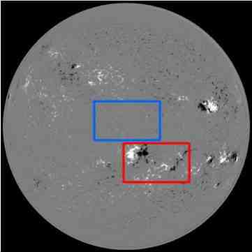
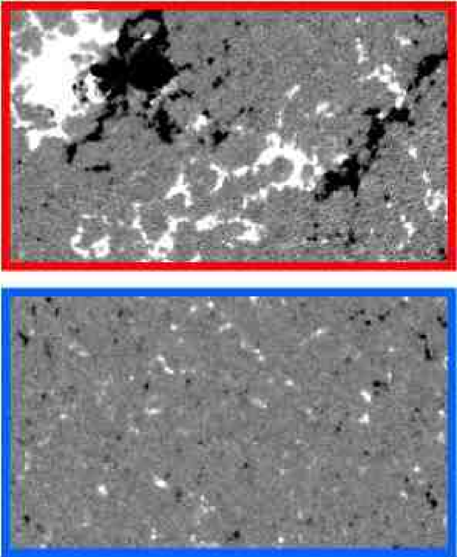
All the solar surface is characterized by a magnetic field with a mixed polarity, but in active regions the unipolar areas are bigger and the magnetic field stronger. This structure is commonly called a magnetic carpet. There is general agreement that the active region field is the direct result of the large-scale solar dynamo. The continuous presence of quiet-sun regions also during solar minima, when the number of active regions considerably decreases, suggests that this flux might be generated by local dynamo action just below the sun’s surface, driven by granular and supergranular flows [55, 18, 74, 51] The opposite polarity regions of the magnetic carpet are connected by closed magnetic field lines, extending up to the upper layers of the solar atmosphere, called loops. In correspondence of active regions, where the magnetic field is stronger, these loops shine bright in EUV and x-rays as shown in Fig. 5
The intimate relationship of the magnetic field and the structures of the outer atmosphere is illustrated in Figure 6 that shows images of the Sun at different wavelengths, corresponding to different temperatures and layers.

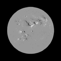
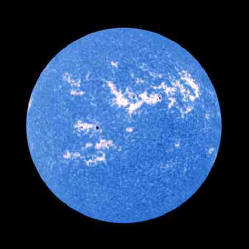
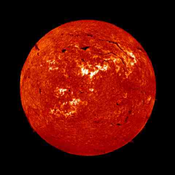
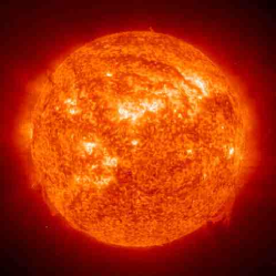


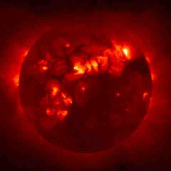
In particular the blue continuum image 6a shows the photosphere, image 6b is a magnetogram showing the line-of-sight component of the magnetic field (white for out-going directed field, black for in-going field), the upper photosphere shown in the light of Ca II K in image 6c, the chromosphere in line in image 6d, the transition region in the light of He II at 304 Å in image 6e, and then the corona seen in lines Fe IX 171 Å formed at in 6f, Fe XII 195 Å at in 6g, Fe XV 284 Å at in 6h, and in the soft x-ray region in 6i. The main information we have from these pictures is the correspondence between the regions of strong magnetic field at the photospheric level (6b) and the activity in all the upper layers of the solar atmosphere up to the X-ray corona. The main structures seen in Figure 6a are the sunspots. Emergence of the magnetic field at the photosphere 6b occurs in and near the spots and elsewhere. The upper photosphere 6c, chromosphere 6d, and transition region 6e show local brightening, heating, at the locations of strong magnetic field. The coronal images 6f-6i show a complex of loops. Note that all space is not covered by loops and that hotter temperature loops tend to be nested inside loops of cooler temperatures.
3 Overview of Coronal Heating Models
In the 1930s Edlen, Grotrian, and Lyot established that the solar corona has a temperature of the order of . After this, the fundamental step was done in the 1940s by Biermann [4], Alfvén [1], and Schwarzschild [83], who pointed out that the high temperatures of the corona are a direct consequence of the convective motions at the photospheric level. The convection does a mechanical work, which subsequently is transported and dissipated in the chromosphere and the corona.
As pointed out in the previous paragraphs, the solar corona consists of magnetically confined regions characterized by closed structures (loops) roughly located around the equator, and regions of “open” magnetic field (coronal holes) roughly located around the northern and southern poles. Observations of the solar corona in EUV and X-rays show that great part of this emission takes place in the closed structures. This is the reason for which the “open” magnetic regions, which look faint in this high-energy range of the spectrum, are called coronal holes. In fact they look like “holes” in an otherwise bright corona.
Whether the mechanism which heats open and closed magnetic regions may be similar or not, in this work we focus our attention on the magnetically confined regions of the solar corona.
The active X-ray corona has a temperature of , an electron and proton numerical density of about , and is magnetically confined in the gauss magnetic field of active regions. These high temperatures are maintained by a heat input of about [95].
In the 1940s Biermann, Alfvén, and Schwarzschild supposed that waves, generated at the photospheric level by convective motions, and then propagating upward into the corona, would have dissipated their energy leading to the high temperatures observed. Although the mechanisms which are able to transfer, store and dissipate the energy are still a matter of debate, the basic idea remains unchanged. The waves which are generated at the photospheric level include sound waves, gravitational waves, and magnetohydrodynamics waves. More recently it has been shown [64, 87, 90, 78] that all but Alfvén waves are dissipated and/or refracted before reaching the corona. Then, while these other waves contribute to chromospheric heating, it is only Alfvén waves which are able to reach the corona.
The Alfvén wave is a purely magnetohydrodynamic phenomenon, and it is essentially an oscillation due to magnetic field line tension. In fact transverse motions of the magnetic field lines cause a force that tries to restore them to straight-line form. Linearizing the equations of magnetohydrodynamics (hereafter MHD) in the simple case of a homogeneous plasma embedded in a homogeneous magnetic field , Alfvèn waves are found as a transverse incompressible wave, propagating in the direction of the wave vector with the dispersion relation:
| (1) |
where is the wave frequency, the Alfvén velocity, the wave vector modulus and is the angle between the magnetic field and the wave vector . Alfvén waves due to photospheric motions are expected to have periods comparable to the 300 seconds characteristic time of granules, whose characteristic dimension is of the order of and their velocity is of the order of . Shorter periods have been detected, but at noticeably reduced power levels.
Coronal loop length is of the order of km, with a typical sound speed of the order of , and Alfvén speed roughly 10 times larger, . An important parameter in plasma physics is the ratio between kinetic and magnetic pressure , that in the case of a coronal loop is of the order of , i.e. a coronal loop is a magnetic dominated system.
The basic problem with wave heating is that the wavelengths of an Alfvén wave with a period typical of photospheric motions are too large to match coronal loop lengths. In fact from the dispersion relation (1) (with ), for a period it follows a wavelength , which is of the same order as the length of the longest loops. Then they are quasi-static displacements of the magnetic fields rather than waves.
Traditionally the mechanisms responsible for coronal heating have been divided into two main groups: AC (alternate current) and DC (direct current).
1 High Frequency Models
AC heating models propose two different mechanisms, Phase mixing (Heyvaerts & Priest [43]) and resonant absorption (Davila [15]), in order to facilitate dissipation of these waves within about one wave-period. They both occur when Alfvén velocity is not uniform.
Phase mixing occurs when Alfvén waves propagate at different phase velocities along nearby fieldlines, making them come out of phase.
Resonant absorption occurs whenever the Alfvén velocity is nonuniform (e.g. if density is not uniform) in a loop cross section. The wave amplitude is enhanced in a narrow layer where the local Alfvén resonance frequency matches the frequency of the global loop oscillations. Gradients in the magnetic and velocity fields are very large in this layer, and the wave energy is easily dissipated by Ohmic and viscous processes.
2 Low Frequency Models
Alternatively it has been proposed (Parker [68], [69], [70], [71]) that the X-ray corona is heated by dissipation at the many small current sheets forming in a coronal loop as a consequence of the continuous shuffling and intermixing of the footpoints of the field in the photospheric convection. The formation of these current sheets is conjectured by Parker [72] in the following way. Consider a region , embedded in a uniform magnetic field aligned along the z-direction . Top and bottom boundaries are located at the planes and . Supposing that in the plane we have a zero velocity field, and that in an incompressible 2-D, i.e. , velocity pattern. A continuous mapping of the footpoints velocity pattern in the perpendicular magnetic field () is produced. This field spontaneously produces tangential discontinuities: the discontinuities appear in the initially continuous field at the boundaries between local regions of different winding patterns. The tangential discontinuities (current sheets) become increasingly severe with the continuing winding and interweaving, eventually producing intense magnetic dissipation in association with magnetic reconnection. Parker suggested that this dissipation is largely in the form of bursts of rapid reconnection. It is this sporadic explosive dissipation at the tangential discontinuities in the bipolar fields on the sun that creates the active X-ray corona. The heating occurs in bursts, which are estimated to involve individually . Such a burst is too small to be observable and he refers to the individual burst as a “nanoflare”, because it is 9 orders of magnitude smaller than a large flare of .
He eventually computes the energy input. Magnetic field lines connect the fixed footpoints at with the moving ones in , which move about with the velocity pattern imposed. The field lines have more or less a uniform deviation to the vertical, where
| (2) |
supposing . The vertical component of the field is , indicating with the orthogonal component we have
| (3) |
the field line tension opposes this movement with a stress of the order of , so that the work for unitary time and surface (the power) done by the photosphere is
| (4) |
The input flux then increases linearly with time. We know from observations that the input flux is of the order of . For a magnetic field , a velocity field , and a loop length , it follows from equation (4) that the observed input flux is reached at , when and (the so-called “Parker angle”). At this point it is conjectured that bursty rapid reconnection dissipates as rapidly as it is produced by the velocity forcing at the photosphere. In this way the input energy flux is on the average always of the order of .
Chapter 1 The Reduced MHD Model for Coronal Heating
A coronal loop (Figure 1) is a closed magnetic structure threaded by a strong axial field, with the footpoints rooted in the photosphere. This makes it a strongly anisotropic system; the measure of this anisotropy is given by the relative magnitude of the Alfvénic velocity compared to the typical photospheric velocity . So the photospheric velocity, that is the amplitude of the Alfvén waves that are launched into the corona, is very small compared to the axial Alfvén wave velocity.

To investigate the properties and dynamics of a so complex system such as a coronal loop, we make a simplified model which captures the essential features of a real loop. The main (indeed defining) feature of a loop is its strong axial field which serves as a guide for the Alfvén waves excited by photospheric motions. It is just the dynamics of these waves, propagating along the guide field, that we want to study. We first assume a simplified geometry, neglecting any curvature effect, and model a coronal loop as a “straightened out” cartesian box (Figure 1), i.e. as a parallelepiped with an orthogonal square cross section of size , and an axial length embedded in an axial homogeneous uniform magnetic field . For a quantitative numerical study, we next adopt the so-called “reduced MHD” equations to model the dynamics of the plasma (Kadomtsev & Pogutse [46], Strauss [88] and Montgomery [58, 59]). Magnetohydrodynamics (MHD) is used to study long-scale low-frequency phenomena in plasma physics. When a plasma is embedded in a strong magnetic field, a further simplified set of equations (“reduced”) are derived from the full set of MHD equations, to model the dynamics of the plasma.
In § 1 reduced MHD equations will be described in detail. In § 2 we give a brief review of current anisotropic MHD turbulence theory, a phenomenon naturally arising in an anisotropic environment such as a coronal loop threaded by a strong axial magnetic field. At last, in § 2 we describe the numerical parallel code that we have developed to solve the reduced MHD equations and that we have used to perform our numerical simulations.
1 Reduced Magnetohydrodynamics
The equations of reduced MHD have been derived in two different research fields. Kadomtsev & Pogutse [46] and Strauss [88] have derived these equations in the context of fusion research to model the dynamics of a plasma embedded in a strong magnetic field. They were specifically thinking about tokamaks, but their derivation is not strictly limited to the geometry of these devices. Montgomery [58, 59] has derived, in a different way, the same set of equations to study MHD turbulence in the presence of a strong magnetic field.
The equations derived by all these authors are exactly the same. This is a clear indication that when a plasma is embedded in a strong axial magnetic field the turbulence which naturally develops is strongly affected by the magnetic field, acquiring its anisotropic features (Montgomery [58, 59], Shebalin et al. [84]), and that the overall dynamics is well described by the equations of reduced MHD (Kadomtsev & Pogutse [46], Strauss [88]). We now derive these equations following Montgomery [59].
The equations of incompressible resistive MHD are:
| (1) | |||
| (2) | |||
| (3) | |||
| (4) | |||
| (5) |
where is a constant and uniform mass density, is the velocity field, the magnetic field, the electric current, the kinetic pressure, the speed of light. Using a simplified diffusion model, both the magnetic resistivity () and the shear viscosity () are constant and uniform.
We now derive the set of equations for a plasma embedded in a strong magnetic field directed along the axial direction . Let’s suppose the following ordering for the magnetic field:
| (6) |
where
| (7) |
We also suppose that gradient scales along the axial field direction are longer than perpendicular scales , an hypothesis which is actually one of the main results of modern anisotropic turbulence theory (see § 4). We introduce similar expansions for velocity, electric current and kinetic pressure:
| (8) | |||||
| (9) | |||||
| (10) |
Using as variables , and , the gradient operator can be written as
| (11) |
The magnetic field is expressed in terms of the vector potential :
| (12) |
with
| (13) |
and we choose the Coulomb gauge for its algebraic convenience.
Introducing the expansion (12) in the equation (2) for the magnetic field, after a few algebraic manipulations we obtain:
| (14) |
where is a scalar potential, resulting from pulling off a curl operator from eq. (2), for which we assume an expansion of the form
| (15) |
The momentum equation (1) becomes:
| (16) |
Considering the leading order contributions from (14), (15), (16), and from (3), (5) we have
| (17) | |||
| (18) | |||
| (19) | |||
| (20) |
Setting , (17) gives
| (21) |
Equation (18) implies that the has only the component along the axial direction
| (22) |
This with equation (20) implies that also has vanishing orthogonal components
| (23) |
Consequently from (12) for we have
| (24) |
so that has a vanishing axial component .
Considering the terms in (14) we have
| (25) |
Introducing the vorticity , and following the above expansion conventions, we have
| (26) |
After some algebra the terms of equation (16) can be written as
| (27) |
Finally, considering the -components of equations (25) and (27), we obtain the reduced MHD equations:
| (28) | |||
| (29) |
Finally, from of equation (19) we have
| (30) |
and considering the orthogonal component of equation (25)
| (31) |
From this last equation it follows , which inserted in (30) implies that, in the absence of a parallel flow at the boundaries, we have
| (32) |
1 Dimensionless Form and Boundary Conditions
The equations of reduced MHD (28)-(29) written for the transverse fields and in dimensional form are:
| (33) | |||
| (34) | |||
| (35) | |||
| (36) |
where is a constant and uniform mass density. To render the previous equations in dimensionless form, we notice that the magnetic fields and can be expressed in velocity dimensions by dividing by , i.e. considering the Alfvénic velocities. As characteristic quantities we use the perpendicular length of the computational box , the typical photospheric velocity , and the related crossing time . The dimensionless equations are then given by:
| (37) | |||
| (38) | |||
| (39) | |||
| (40) |
where is the ratio between the axial Alfvénic velocity and the photospheric velocity, i.e.
| (41) |
and
| (42) |
are the kinetic and magnetic Reynolds numbers.
Introducing the velocity and magnetic potentials and
| (43) |
| (44) |
| (45) |
equations (37)–(38) in terms of potentials are written as:
| (46) | |||
| (47) |
where the poisson bracket of two functions and is defined as:
| (48) |
Using equations (43) it can be shown that:
| (49) |
Using these relations, equations (46)-(47) can be rewritten as:
| (50) | |||
| (51) |
In turbulence theory the fundamental variables are the Elsässer variables
| (52) |
in terms of which, and supposing the Reynolds numbers to have the same values , the reduced MHD equations (37)-(40) are:
| (53) | |||
| (54) | |||
| (55) |
where is the total pressure, and is linked to the nonlinear terms by incompressibility (55):
| (56) |
An analysis of equations (53)-(55) gives us a qualitative preview of the results which will be obtained both numerically and analytically in the following chapters. The linear terms in equations (53)-(55)
| (57) |
show that fields present an Alfvén wave propagation along the axial field direction. In particular describes waves propagating in the direction of , and in the opposite direction; both at the Alfvén wave velocity . This wave propagation is present also when the nonlinear terms become important, and transport energy from the photospheric boundaries into the system.
As boundary conditions at the photospheric surfaces () we impose a velocity pattern which mimics photospheric motions. In terms of the Elsässer variables the velocity is the sum
| (58) |
In terms of characteristics this gives rise to a “reflection” of the Alfvén waves at the boundaries, where we can only impose a condition on the incoming wave (alternately and ). To mimic photospheric motions we impose a velocity pattern on the top and bottom planes. In terms of the Elsässer variables to impose a velocity pattern means using the constraint
| (59) |
Since and are, respectively, waves propagating toward the inside and the outside of the computational box, this is a “reflection” condition on these waves, i.e.
| (60) |
| (61) |
At the boundary the value of the incoming wave is equal to the negative value of the outgoing wave plus twice the value of the velocity at the photosphere.
A fundamental feature of the nonlinear terms (and also the pressure term (56)) is the absence of self-coupling, i.e. the nonlinear interaction depends by the counter-propagating fields , and if one of the two fields were zero there would be no nonlinear dynamics at all. This is the basis of the so-called Alfvén effect, which is described in § 2, and is the basis of anisotropic turbulence phenomenology.
2 Conservation Laws
MHD theory provides a number of conservation laws which play an important role in turbulence theory. We are mainly interested in the Energy, Cross Helicity, and Magnetic Helicity. Turbulence is usually studied with the hypothesis of periodicity in all three spatial directions. In our case along the direction of the axial field this condition breaks down. The flux terms which are usually neglected become important. In this paragraph we write the conservation laws for the three aforementioned quantities, including the flux terms and restricting our attention to the reduced MHD equations.
Multiplying the momentum equation (37) by and the magnetic field equation (38) by we obtain:
| (62) | |||
| (63) |
On the other hand from
| (64) |
it follows that
| (65) | |||
| (66) | |||
| (67) |
In this way equations (62)-(63) can be rewritten as
| (68) | |||
| (69) |
The first term between square brackets in the right hand side of equation (68) is orthogonal to and hence its scalar product with is zero. Furthermore
| (70) |
and
| (71) |
| (72) |
We can now write for the energy density, summing equations (68) and (69)
| (73) |
The following relations hold:
| (74) |
| (75) |
| (76) |
where
| (77) |
We can now write
| (78) |
The Poynting Flux is given by:
| (79) |
So using equation (64) we have
| (80) |
and the component along the axial direction is
| (81) |
At last we can write
| (82) |
Calling the total Energy , the Ohmic dissipation rate , and the viscous dissipation rate (which is the enstrophy divided by the Reynolds number )
| (83) | |||||
| (84) | |||||
| (85) |
and the integral of the Poynting flux given by
| (86) |
where the signs have been chosen so that is positive when we have energy entering the system and negative when it leaves. We can write the integral of equation (82)
| (87) |
Another important conserved quantity is cross helicity , defined as:
| (88) |
Multiplying the momentum equation (37) by and the magnetic field equation (38) by , after a few algebraic manipulations we obtain
| (89) |
When taking the integral over the volume the first and second terms in square brackets do not contribute because their only components lie in the orthogonal plane where we have periodic boundary conditions. But the third term cannot be neglected and we thus obtain
| (90) |
Given a magnetic field and its vector potential for which , in MHD the magnetic helicity is usually defined as
| (91) |
but this definition is, in general, not gauge invariant. In fact taking a gauge transformation gives
| (92) |
Now equation (91) is gauge invariant, but only when the surface integral (92) vanishes. This condition is satisfied when the normal component of the magnetic field vanishes at the boundary surface. For our coronal loop this condition does not apply, and definition (91) cannot be used. An alternative expression has been proposed by Finn and Antonsen [25] (see also Berger and Field [3])
| (93) |
where is a reference field to be chosen suitably. To satisfy gauge invariance and should have the same normal component at the surface boundary.
In the reduced MHD case we show that, even if it were possible to give a gauge invariant definition of the magnetic helicity, it would not have a physical meaning. In reduced MHD the field is decomposed as , where is constant and uniform. We choose the vector potential and . We have only 4 terms which may contribute to an expression like (93), but only one of them is not null. In fact
| (94) | |||
| (95) | |||
| (96) | |||
| (97) |
Integrating over the volume equation (95) vanishes because of the periodic boundary conditions of , so only equation (97) does not vanish. On the other hand, when integrating over the volume, this term is the zero frequency component of , i.e. a constant which can always be subtracted through a gauge transformation.
In full ideal MHD magnetic helicity is a conserved quantity, but in reduced MHD it does not seem to have a physical meaning. While in 2D MHD magnetic helicity is zero but any moment of is conserved, in reduced MHD this does not apply. We rewrite for convenience equation (46) with :
| (98) |
When the derivative term is zero, this equation becomes the 2D MHD equation, and it easily follows that any moment of is conserved when . In the reduced MHD case the divergence gives a vanishing contribute (as it does for 2D MHD):
| (99) |
because the normal component of the velocity is zero at the photospheric surfaces, and the remaining boundary surfaces are periodic. The presence of the derivative term breaks the conservation of , except for , but in this case it is again a function which can be subtracted from through the gauge transformation
| (100) |
so that for
| (101) |
2 Anisotropic MHD Turbulence
Wherever a fluid is set into motion turbulence tends to develop. When the fluid is electrically conducting, turbulent motions are accompanied by magnetic field fluctuations. Although plasmas are abundant in the universe (it is said that 99% of the baryonic material in the universe is in the plasma state), conducting fluids are rare on earth, where electrical conductors are usually solid. Hence it is not surprising that magnetohydrodynamic turbulence (Biskamp [5]) has received attention only recently, after that hydrodynamic turbulence has been studied at length (Frisch [29]).
A milestone in turbulence theory is the work by Kolmogorov [47] on the scaling properties of hydrodynamic turbulence, where he finds the well-known power spectrum for total energy. The presence of the magnetic field strongly affects the properties of turbulence. While it is possible through a Galilean transformation to subtract a mean (or local) velocity field, this transformation has no effect at all on the magnetic field (a mean global or a local one).
Since the pioneering work of Iroshnikov [45] and Kraichnan [48] (hereafter IK) there has been a lot of debate on which are the main properties of MHD turbulence. The Alfvén effect, which arises from the fact that only oppositely propagating Alfvén waves interact, and the hypothesis of homogeneity and isotropy lead to a scaling for the energy spectrum, which differs from the Kolmogorov scaling in the hydrodynamic case (Kolmogorov [47], Obukhov [63]).
The anisotropy of MHD turbulence is one the properties characterizing the recent debate (Shebalin et al. [84], Sridhar & Goldreich [86], Goldreich & Sridhar [33], Montgomery & Matthaeus [60], Goldreich & Sridhar [34], Cho & Vishniac [11], Maron & Goldreich [54], Cho et al. [10]). There is broad agreement that the anisotropy of MHD strongly affects its properties, simply due to the presence of a magnetic field, and that the hypothesis of homogeneity and isotropy must be relaxed.
Shebalin et al. [84] have shown that the energy cascade takes place mainly in the plane orthogonal to the static (DC) magnetic field, while it is weaker in the parallel direction. Sridhar & Goldreich [86] and Goldreich & Sridhar [33, 34] have shown that the anisotropy gets stronger at large wave-numbers, i.e. whilst the cascade takes place. These results have been numerically investigated and confirmed by Cho & Vishniac [11], Cho et al. [10].
1 Turbulent Cascade and Phenomenology of the Inertial Range
A characteristic property of fully developed turbulence is the presence of a broad range of different scales. Relevant physical quantities, such as energy, are excited within a certain spectral range , called the injection scale. Nonlinear interactions transfer these quantities in -space towards larger wavenumbers up to the dissipation scale , where a dissipative physical process is supposed to act as a sink for this energy flux.
The region in Fourier space between the injection and the dissipation scale
| (102) |
is called the ‘inertial range’. In this spectral range the turbulence develops solely under the influence of the internal nonlinear dynamics without being directly influenced by either the external injection of energy or by dissipative processes. Spectra in the inertial range exhibit power-laws, and the inertial range can be defined as the wavenumber range within which the spectrum has a power-law behavior.
What we have just described is called a direct cascade, but sometimes a flux of energy in the opposite direction occurs, i.e. from the injection scale towards smaller wavenumbers. This process is called inverse cascade, and when it occurs a second inertial range, besides (102), is found
| (103) |
The lower limit is usually determined by the size of the system .
We now briefly summarize the Kolmogorov phenomenology of the inertial range (K41). We explicitly consider the case of a direct cascade and of an isotropic system. The results that we will describe in the next chapter depart substantially from the K41 theory, but many concepts, ideas and notations are used also in anisotropic turbulence theory. Considering isotropic turbulence we can define the angle-integrated spectra in the following way:
| (104) |
where thanks to isotropy we consider only the scalar wavenumber .
The dynamics of turbulence is controlled by the rate at which energy is injected into the system at the injection scale , it is subsequently scattered along the inertial range with the transfer rate , and finally swept away from the system at the dissipation scale with the dissipation rate . For stationary turbulence all these spectral energy fluxes are equal
| (105) |
This equality still holds approximately when the injection energy rate changes in time, because the more rapid dynamics at the small scales in the inertial and dissipation ranges adjust the spectrum rapidly compared to the slower dynamics of the large scales. For convenience we divide the inertial range into a discrete number of scales ,
| (106) |
and the division is taken on a logarithmic scale , where is of the order of the large scale . The time taken for the transfer of energy between two neighboring scales and is given by , the so-called eddy turnover time of the eddy , for simplicity
| (107) |
Since the energy flux is constant across the inertial range, we can write
| (108) |
From this equality we can find the scaling
| (109) |
To obtain the energy spectrum we identify the eddy energy with the band-integrated Fourier spectrum
| (110) |
from which we obtain, substituting , the Kolmogorov spectrum
| (111) |
We remark again that the hypothesis of isotropy has been essential to obtain the K41 spectrum (111).
2 The Alfvén Effect
In the hydrodynamic case isotropy is normally justified, but for plasmas a magnetic field is always present. This introduces an anisotropy of the system which cannot be eliminated.
Four decades after Iroshnikov [45] and Kraichnan [48] presented their ideas on MHD turbulence, the debate on which physical mechanisms drive it is still active. Rewriting the equations of incompressible MHD (1)-(5) expressing magnetic field in velocity units, i.e. , and making them non dimensional choosing a characteristic velocity , a characteristic length , and the related crossing time , we have in terms of the Elsässer variables :
| (112) | |||
| (113) |
where we assumed the kinetic () and magnetic () Reynolds numbers, defined as
| (114) |
to be equal (). is the total pressure in dimensionless form, and it is tied to the fields by incompressibility (113):
| (115) |
In the following analysis we ignore the dissipative terms, because dissipation provided by , supposed it has a high value, takes place only at small spatial scales. A constant and uniform magnetic field in absence of fluid motions:
| (116) |
is a homogeneous solution of equations (112)-(113). A linear analysis of incompressible MHD shows that we have only Alfvén waves, in particular linearizing equations (112)-(113) with the equilibrium (116) yields:
| (117) |
Equations (117) show that describes Alfvén waves propagating toward positive at the speed , and describes Alfvén waves propagating at the same speed but in the opposite direction. A notable property of the Elsässer fields in equations (112)-(113) is the absence of self-coupling in the nonlinear term. In fact there is only cross-coupling of and . This property allows for a nonlinear generalization of the linear Alfvén waves described by equations (117). Singling out the equilibrium (116) ( in terms of Elsässer variables)
| (118) |
and requiring the generalized Alfvén wave to retain its transversality, i.e. , we have for the nonlinear term
| (119) |
This means that if one of the two Elsässer fields is zero the nonlinear term in equation (119) vanishes and equations (112)-(113) assume the linear form (117) for the remaining Elsässer field, even if its amplitude is not small. If at some time, like , and from equations (117) we have that the solution is , . If at time we had and , then the solution would be and . These nonlinear solutions are Alfvén wave packets of arbitrary form propagating nondispersively in the direction of the main field , and in the opposite direction. The dynamics are very simple as long as there is no spatial overlap (“collision”) between two oppositely moving packets and . Hence only Alfvén waves propagating in opposite directions along the guide field interact. This is the basis of the Alfvén effect introduced independently by Iroshnikov [45] and Kraichnan [48] who noted that the cascade of energy in MHD turbulence occurs as a result of collisions between oppositely directed Alfvén wave packets. This result is quite general for MHD, in fact the guide field need not be an external static field, but can also be the field in the large-scale energy-containing eddies.
3 The Iroshnikov-Kraichnan Formulation
To derive the results of IK theory we consider a statistically steady, isotropic excitation of amplitude , at the injection scale of the equilibrium defined by equations (116). The turbulent cascade produces Alfvén wave packets at scales traveling in opposite directions along the large-scale field. A fundamental hypothesis made by both Iroshnikov [45] and Kraichnan [48] is that the energy transfer in Fourier space is local and isotropic. At this point we restrict the discussion to weak velocity-magnetic-field correlation , which is the condition that applies to our model for a coronal loop and that we will discuss in more detail in the next chapter.
We distinguish between two important dynamical time scales, the time for distortion of a wave packet at scale by a similar eddy , i.e. the eddy turnover time
| (120) |
and the Alfvén time , which is the interaction time of the two oppositely moving wave packets. In general , so the interaction time of the two wave packets is much shorter than the non-magnetic eddy turnover time . The change in amplitude is small during a single collision of two wave packets since it is proportional to the interaction time:
| (121) |
During successive collisions these perturbations add with random phases and, given the diffusive nature of the process, the number of collisions for the small perturbations to build up to order unity (i.e. ) is
| (122) |
The energy-transfer time , which in hydrodynamic turbulence is just , is longer
| (123) |
Making the substitution in equation (108) we obtain for the spectral energy flux
| (124) |
From this we get the scaling
| (125) |
and identifying the eddy energy with the band-integrated Fourier spectrum (where ) we obtain the Iroshnikov-Kraichnan (IK) spectrum for MHD turbulence
| (126) |
which is less steep than the Kolmogorov spectrum (111). Using the scaling (125) in (122) we obtain for the number of collisions per energy transfer time:
| (127) |
As we proceed along the cascade toward smaller scales the number of collisions required for the fractional perturbations to build up to order unity increases, verifying the hypothesis (121) that we made at the beginning. Furthermore, during each collision the fraction of energy that cascades gets smaller with decreasing scale; in fact, from equations (121) and (122) we have that
| (128) |
In this sense we say that the cascade “weakens” at large wavenumbers.
4 Beyond IK: Fully Anisotropic MHD Turbulence
Isotropy is the underlying hypothesis used in the IK derivation of turbulence scaling properties (120)-(128). In particular we have imposed the condition that the wave packets are isotropic on the length-scale , also along the direction of the equilibrium magnetic field .
Only later it has been understood that the anisotropy due to the presence of the main axial field not only acts through the Alfvén effect, but has also a deep impact on the nonlinear dynamics, producing two different behaviors along the direction of the main field and in the orthogonal plane (Shebalin et al. [84], Sridhar & Goldreich [86], Goldreich & Sridhar [33], Montgomery & Matthaeus [60], Goldreich & Sridhar [34], Cho & Vishniac [11], Maron & Goldreich [54], Cho et al. [10]).
Shebalin et al. [84] used the reduced MHD equations (46)-(47) to numerically investigate the cascade properties of a 2D turbulent system embedded in a strong field directed along the -axis, considering the system invariant along the -direction, so to perform 2D numerical simulations in the - plane. As initial conditions they considered wave packets with an isotropic spectral distribution in the - plane, as in the IK theory, so that the isocontours of the spectral densities were circles at the beginning of the simulation. They found that the spectrum evolves anisotropically by transferring energy to modes perpendicular to far more rapidly than to modes with parallel to . In this way the initially circular spectral density contours elongated in the perpendicular direction. Even if it was not initially valid, the evolution proceeded toward the reduced MHD approximation. Even if the simulation was started with an isotropic initial condition, the temporal evolution was strongly anisotropic.
The isotropic hypothesis used for the IK phenomenology (120)-(128) is therefore neither consistent nor correct, as pointed out by Sridhar & Goldreich [86] and Goldreich & Sridhar [34]. In this sense Iroshnikov [45] and Kraichnan [48] have only partially implemented the consequences of anisotropy in MHD turbulence through the Alfvén effect, but the full consequences of anisotropy have been understood only later, and its elucidation is not yet complete.
To understand why perpendicular transfer is easier we present a simplified perturbative argument in order to estimate possible energy transfer between Alfvén wave modes. Introducing in incompressible MHD equations (112)-(113) the expansion
| (129) |
where is the homogeneous equilibrium (116), and are Alfvén waves of the form
| (130) |
where , and . Noting that from equation (115) the pressure gradient term has only second order terms, i.e.
| (131) |
at the second order we have
| (132) |
This equation has basically the same structure of the wave equation for , except for an effective driving term on the right, due to the linear Alfvén waves (130).
The most efficient mechanism for fast energy transfer between modes is resonant interactions occurring among triads of modes with wavenumbers , and related by the conditions
| (133) |
where . Shebalin et al. [84] noted that the only nontrivial solution of (133) requires that the -component of one member of the triad, e.g. , must be zero. This implies that waves with values of not present initially cannot be created during collisions between oppositely propagating wave packets. Hence there is no parallel, i.e. along , cascade of energy. Energy will cascade to large wavenumbers in the orthogonal plane , making the turbulence cascade anisotropic.
We can now derive the anisotropic version of the IK theory (120)-(128), taking into account that there is no cascade along the direction of the main magnetic field . We suppose again that the system is excited at the scale in a statistically steady and isotropic fashion such that . The absence of a parallel cascade implies that wave packets belonging to the inertial range have parallel scales and perpendicular scales . As previously supposed by IK, the Alfvén effect takes place and only counter-propagating wave packets interact. The wave packets are “long-lived” and they need many collisions to loose a significant amount of energy. We distinguish again between the eddy turnover time characterizing the cascade in the orthogonal plane,
| (134) |
where , and the Alfvén time , which is the interaction time of two oppositely propagating wave packets and . Now, because of the absence of cascade along , the Alfvén time is scale-independent, i.e. it does not depend on the scale :
| (135) |
The interaction time is still small compared to the eddy turnover time , so the energy loss of the eddy at the scale is small during a single collision
| (136) |
The number of collision that a wave packet at the scale must suffer for the fractional perturbation to build up to order unity is now
| (137) |
The energy-transfer time is again given by
| (138) |
while for the energy flux we have
| (139) |
From the previous equations we obtain the following scaling relation
| (140) |
and identifying the eddy energy with the band-integrated Fourier spectrum (where ) yields the anisotropic version of the IK spectrum for MHD turbulence
| (141) |
which exhibits the characteristic spectral index. Another difference with the IK formulation is given by the behavior of the number of collisions at small scales:
| (142) |
Contrary to IK, decreases with decreasing . When the number of collisions decreases at small scales we say that the turbulence “strengthens”. At a small enough scale the conditions (136)-(137) will not be satisfied, thus limiting the spectral range in which the spectrum applies.
Weak perturbation theory (Zakharov et al. [96]) deals with the effects of the nonlinear terms in equations (112)-(113) in a systematic, perturbative manner. When the nonlinear terms are ignored, the Fourier amplitudes and phases of the waves are constant in time. However, the nonlinearity makes the amplitudes change slowly over many wave periods. It is this slow change in the amplitudes that determines energy transfer among the linear modes. A kinetic equation for the rate of change of energy in a mode with wave-vector describes how other modes in the system affect the energy in this mode. To lowest order in the nonlinearity, the kinetic equation takes into account the interactions among modes taken three at a time, as shown in (133). When equations (133) is satisfied, one says that a 3-wave resonant interaction is allowed. When 3-wave resonant interactions are forbidden, because the 3-wave resonant coupling coefficients vanish, the effects of 4-wave resonant interactions must be considered.
Goldreich & Sridhar [34] showed that although the anisotropic IK formulation (134)-(142) describes a weak turbulence, in the sense that the fractional change in wave amplitude during each wave period is small, strains in the fluid are so strong that perturbation theory diverges. It turns out that not only 3-wave interactions contribute, but also higher order terms. At lowest order in perturbation theory, wave packets move along field lines. Thus the breakdown of perturbation theory can be understood physically by studying the geometry of the divergence of a bundle of field lines. Assume that the mean field lies along the direction, and consider wave packets with longitudinal scale , and transverse scale , with . For the turbulence to be weak we require the condition (136) to be satisfied, i.e.
| (143) |
so that . The rms inclination of the local field is , so that after a single collision between two wave packets taking place along the longitudinal scale , the wave packet will suffer an orthogonal displacement . Given the diffusive nature of the process after collisions the wave packet has traveled a distance in the longitudinal direction, suffering an rms orthogonal displacement
| (144) |
The distance along over which increases by a factor of order , i.e. , is
| (145) |
The perturbative expansion converges if the energy spectrum is cut off at small wavenumbers, below (Sridhar & Goldreich [86], Goldreich & Sridhar [34]). In this case it is shown that 3-wave resonant contributions vanish and 4-wave interactions must be considered. For a system with a finite longitudinal extension , such as a coronal loop, this means that for a sufficiently weak perturbation , we move from the anisotropic IK phenomenology (134)-(142) to a new one based on 4-wave resonant interactions that we now briefly describe. The elementary interactions involve scattering of two waves:
| (146) |
Using and the -component of the equation for conservation, Sridhar & Goldreich [86] proved that this scattering process leaves the ’s components unaltered. This implies that waves with values of that are not present in the external stirring cannot be created by resonant 4-wave interactions. The absence of a parallel cascade implies that wave packets belonging to the inertial range have parallel scales , and perpendicular scales . The phenomenology of this new cascade based on 4-wave interactions is very similar to the anisotropic IK phenomenology describe by equations (134)-(142), and can be derived in the same way with a few modifications. The Alfvén effect takes still place, so that only counter-propagating wave packets interact, and the wave packets need many collisions to loose energy significantly. The eddy turnover time and the Alfvén time are defined in the same way (see equations (134) and (135)) and have the same meaning, but now the fractional loss is different from what computed in (136), and from perturbation theory (Sridhar & Goldreich [86], Goldreich & Sridhar [34]) we have that:
| (147) |
The number of collision that a wave packet at the scale must suffer for the fractional perturbation to build up to order unity is now
| (148) |
so the energy-transfer time is
| (149) |
and for the spectral energy flux we obtain
| (150) |
From the previous equations the scaling relation
| (151) |
or equivalently
| (152) |
are obtained. Identifying the eddy energy with the band-integrated Fourier spectrum where we obtain the spectrum for MHD turbulence bases on 4-wave interactions:
| (153) |
As in the case of the anisotropic IK phenomenology (134)-(142) the number of collisions
| (154) |
decreases at small scales and the turbulence becomes stronger.
The previous scalings (134)-(142) and (147)-(154) are based respectively on 3-waves and 4-waves resonant interactions. These scalings can be generalized to the case of single collisions of -waves. The derivation is very similar to what we have already done, and we briefly describe it. We suppose again that the system is weakly excited () at the scale , and that -waves resonant interactions produce a perpendicular cascade. The interaction time is small compared to the eddy turnover time , so that the energy loss of the eddy at the scale is small during a single collision, and is given by (see Goldreich & Sridhar [34])
| (155) |
The number of collisions is now
| (156) |
the energy-transfer time
| (157) |
and the spectral energy flux
| (158) |
From the previous equations we obtain the following scaling relation
| (159) |
or equivalently
| (160) |
and the anisotropic spectrum for MHD turbulence based on single -waves resonant interactions is
| (161) |
The spectral index spans from and for the cases that we have already treated ( and ), and has a lower limit of as . A common feature for the number of collisions
| (162) |
is the “strengthening” of the turbulence at small scales, for all .
A parameter that characterizes weak turbulence is (see eq. (143)):
| (163) |
which, for weak turbulence, is small . At a sufficiently small scale along the cascade the turbulence will get strong enough so that , and just collision (see eq. (156)) with another wave packet of comparable size will result in a fractional change in wave amplitude of order one, i.e. from equations (155)-(156). The same result is obtained if the perturbation at the injection scale is strong enough, i.e. so from eq. (163) we have . In this case wave packets lose their identity after they travel one wavelength along the field lines. Consequently the eddy turnover time and the Alfvénic time are the same,
| (164) |
where , which is called a “critical balance” (Goldreich & Sridhar [33]). Consider an eddy of dimensions and along the directions parallel and orthogonal to the mean magnetic field. Because of the turbulent transfer to smaller perpendicular scales, shrinks and the eddy becomes more elongated, leading to sheet-like structures limited only by dissipation. The spectral cascade takes place mainly in the orthogonal plane with constant energy flux across the inertial range
| (165) |
Combining this relation with equation (164) we obtain
| (166) |
where we define the scale . This relation shows also that this anisotropy increases toward smaller scales, the ratio
| (167) |
gets bigger for larger (smaller ).
For the spectrum the original K41 phenomenology (107)-(111) is valid, with a slight modification to account that the cascade takes place in the orthogonal plane. But this analogy is only formal, because now we discard isotropy; in particular, the Alfvén effect takes place and the cascade occurs mainly in the orthogonal plane. The eddy turnover time and the energy transfer time now are the same
| (168) |
and since the energy flux is constant across the inertial range, we can write
| (169) |
yielding the scaling
| (170) |
So from the band-integrated Fourier spectrum in the orthogonal plane (i.e. with )
| (171) |
we recover the Kolmogorov spectrum
| (172) |
but now only in the orthogonal plane.
Chapter 2 The Numerical Code
A numerical code, written in Fortran 90 and parallelized with MPI, has been developed to solve the non-dimensional reduced MHD equations (46)-(47), that we rewrite here for convenience:
| (1) | |||
| (2) |
The computational domain is a parallelepiped () with an orthogonal (, ) square cross section of size , and an axial () length , with the normalization (because of our choice for the length-scale to render equations dimensionless shown in § 1), and (see Figure 1). In the orthogonal planes ( and directions) periodic boundary conditions are used coupled with a Fourier pseudo-spectral numerical method (Canuto et al. [8]). In the axial direction , a velocity pattern is imposed at the top and bottom boundaries (see equations (60)-(61)), and a central finite difference scheme of the second order is used. Time is discretized with a third-order Runge-Kutta method coupled with an implicit Crank-Nicholson scheme for the diffusive terms.
When investigating turbulence, the diffusive terms provide a sink for the flux of energy at small scales. One of the problems present when performing a numerical investigation is the limitation on the number of grid points. While the Reynolds numbers and have large values in most physical problems of interest, the number of points is necessarily limited when performing a numerical simulation which, in turns, restricts the Reynolds numbers to low values. Thus, diffusion is not limited to small scales, but also affects the large scales. If one of the purposes of the numerical investigation is to study the inertial range behavior, even with a resolution of points in the planes, the inertial range is disturbed by diffusion. In numerical studies of turbulence it is often practical to use higher-order diffusion operators, or hyperdiffusion:
| (3) |
where the exponent is called dissipativity. In this way dissipation is strongly concentrated at the small scales, and the dissipative pollution of the inertial range is avoided. We have performed simulations with both normal diffusion () and hyperdiffusion with dissipativity .
1 Fourier Transform and Spatial Derivatives
Suppose is a complex periodic function of period , defined on a uniformly spaced grid of points:
| (4) |
Indicating with the value of the function at the point , i.e. , the discrete Fourier transform at the wavenumber can be defined as (see Numerical Recipes [77]):
| (5) |
to which corresponds the inverse Fourier transform
| (6) |
Since the only differences between (5) and (6) are changing the sign in the exponential and dividing the result by N, a routine for calculating the discrete Fourier transform can also, with slight modifications, calculate the inverse transform.
Although equation (5), the discrete Fourier transform, seems to be an process (i.e. to compute the values of the function it would require to compute operations), an efficient algorithm called the fast Fourier transform or FFT (Numerical Recipes [77]) requires only operations. The FFT algorithm became generally known in the mid-1960s, from the work of Cooley and Tukey, and nowadays it is broadly used in scientific computing. FFTs are generally available as library subroutines and the focus is mainly on achieving the best possible performance on a computing platform. We have chosen to use the FFTW library (Frigo & Johnson [28], see also http://www.fftw.org), which is Free Software distributed under the GNU General Public License. FFTW is typically faster than other publicly-available FFT implementations and is competitive with vendor-tuned libraries that are tuned to work efficiently on specific CPUs. In this way we have achieved our goal to have a cross-platform portable code with a good performance.
From equations (4) and (6), it easily follows that the spatial derivative computed at the point is given by
| (7) |
Hence, to compute the derivative we first compute the Fourier coefficients , then we multiply them by the factor , and finally we perform the inverse Fourier transform (6) with these modified coefficients. The precision of this pseudo-spectral method is much higher than that of an ordinary finite difference scheme. Even with relatively few grid points the computed value of the derivative is almost exact, with the error mainly due to the precision of the numerical processor (see Canuto et al. [8]).
Time evolution is performed in Fourier space, rather than in coordinate space, so that we solve the Fourier transform of the reduced MHD equations (46)-(47). Extending the notations introduced in (4), (5) and (6) to 2 dimensions, and noting that in our case , we can write for a generic function :
| (8) |
and , are intergers ranging from to . Introducing this expansion for the magnetic and velocity potentials, respectively and , in (46)-(47) we obtain the reduced MHD equations in Fourier space:
| (9) | |||
| (10) |
where and . Note that to compute the Fourier components of the Poisson brackets, e.g.
| (11) |
we must first compute the inverse Fourier transform of and , then calculate the Poisson bracket in real space, and finally obtain its Fourier transform.
When hyperdiffusion (3) is used in Fourier space, the diffusive term is always linear, and the only thing that changes is the power of the -factor:
| (12) |
Since Crank-Nicholson schemes are well-suited for the time advancement of linear terms, time evolution is performed with a third-order Runge-Kutta method (for the nonlinear terms and the -derivatives) coupled with an implicit Crank-Nicholson scheme for the diffusive terms. To prevent numerical instabilities due to aliasing of the solutions, we truncate the Fourier transforms outside a circle of radius in the - plane, where is the number of modes and the resolution in the real domain in the - plane (e.g. equation (8)). For time integration we require that the time-step satisfies the CFL (Courant-Friedrichs-Levy) condition in the - plane as well as in the direction. This check is performed by a subroutine which dinamically adapts the value of the time-step.
2 Message-Passing Interface and Parallel Computing
To investigate some of the most interesting problems in physics, astrophysics, and engineering, challenging numerical computations are required. In numerical studies of turbulence we have already remarked that high grid resolutions are a necessity. For instance, if we had not performed some numerical simulations using hyperdiffusion (3) and a numerical grid with points (these are more than millions grid points! ), most of the conclusions presented in this thesis would have been unattainable.
Serial computers are not suitable to perform this kind of simulation, and it is necessary to use a parallel computing system, i.e. a computer with more than one processor for parallel processing (commonly referred to as high-performance computers or supercomputers). These machines are used to perform numerical simulations of phenomena too complex to be reliably investigated by analytical methods, such as fully nonlinear problems, and/or very difficult or impossible to reproduce in a laboratory (unfortunately such as a coronal loop or most of the astrophysical problems of interest).
There are many different kinds of parallel computers. One major way to classify parallel computers is based on their memory architectures. Shared memory parallel computers have multiple processors accessing all available memory as a global address space. They can be further divided into two main classes based on memory access times: Uniform Memory Access (UMA), in which access times to all parts of memory are equal, or Non-Uniform Memory Access (NUMA), in which they are not. Distributed memory parallel computers also have multiple processors, but each of the processors can only access its own local memory. There is no global memory address space; but the processors communicate with each other through an intercommunication network, which can have many different topologies including star, ring, tree, hypercube, fat hypercube (a hypercube with more than one processor at a node), an n-dimensional mesh, etc.. Parallel computing systems with hundreds of processors are referred to as massively parallel.
The Message Passing Interface (MPI) is a computer communication protocol (see [26, 27, 38, 2], and also http://www.mpi-forum.org). The message-passing model posits a set of processes that have only local memory but are able to communicate with other processes by sending and receiving messages. It is a defining feature of the message-passing model that data transfer from the local memory of one process to the local memory of another requires operations to be performed by both processes. Although the specific communication network is not part of the computational model it is one of the more delicate points in parallel computing, often representing the bottleneck to the performance of a numerical code. The challenge is always to try building intercommunication networks (also called switches) that keep up with speeds of advanced single processors. Faster computers require faster switches to enable most applications to take advantage of them.
MPI is an attempt to collect the best features of many message-passing systems that have been developed over the years and to improve and standardize them. MPI is a library, not a language. It specifies the names, calling sequences, and results of subroutines to be called from Fortran, C and C++ programs. Programs are compiled with ordinary compilers and linked with the MPI library. It is emerging as a standard for communication among the nodes running a parallel program on a distributed memory system, although MPI can also be used on shared memory computers. Its advantage over older message passing libraries is that it is both portable (because MPI has been implemented for almost every distributed memory architecture) and fast (because each implementation is optimized for the hardware on which it runs).
The message-passing model fits well on separate processors connected by a communication network. Thus, it matches the hardware of most of today’s parallel supercomputers. Where the machine supplies extra hardware to support a shared-memory model, the message-passing model can take advantage of this hardware to speed up the rate of data transfer. Message passing has been found to be a useful and complete model in which to express parallel algorithms. It provides control when dealing with data locality and, by controlling memory references more explicitly than any of the other models, the message-passing model makes it easier to locate erroneous memory reads and writes.
But the most compelling reason why message passing will remain a permanent part of the parallel computing environment is performance. As modern CPUs have become faster, management of their caches (divided in many levels) and the memory hierarchy in general has become the key to getting good performance. Message passing provides a way for the programmer to explicitly associate specific data with processes and thus allow the compiler and cache-management hardware to function fully. Indeed, one advantage distributed-memory computers have over even the largest single-processor machines is that they typically provide more memory and more cache. Memory-bound applications can exhibit superlinear speedups when ported to such machines and, even on shared-memory computers, the message-passing model can improve performance by providing more programmer control of data locality in the memory hierarchy.
For these reasons message-passing has emerged as one of the more widely used paradigms for implementing parallel algorithms. Although it has shortcomings, message-passing comes closer than any other paradigm to being a standard approach for the implementation of parallel applications. Message-passing has only recently, however, become a standard for portability. Before MPI, there were many competing variations on the message-passing theme, and programs could only be ported from one system to another with difficulty.
3 Code Parallelization
The numerical code has been developed to solve equations (9)-(10), which are the reduced MHD equations in Fourier space. As already noted in § 1, at each time-step the Fourier transforms of the fields and their inverse transforms must be computed to calculate the Poisson brackets. As shown in (5) and (6) to compute the value of a Fourier transform at one point along a given direction, we must know the values of the function in all grid points along that direction. This makes the Fourier transform an intrisically non-parallel computation. In fact if the values of the function along that direction were assigned to different processors, at each time-step all these processors would have to communicate these values to one processor which would compute the Fourier transform. Communications between processors is not very fast and then we want to minimize it.
Although there are algorithms which parallelize the fast Fourier transform more or less efficiently, as a first step we have avoided this, taking advantage of the fact that we use a finite difference scheme of the second order along the direction. These schemes are very well suited for parallelization, because to compute the value of the derivative of a function in one point we only need to know the values of the function in a few neighboring points. In the case of our central finite difference scheme of the second order only the values of the two neighboring points are required. We have decomposed our computational box, which is a parallelepiped (see Figure 1) of dimensions with a grid of points, into slices along the direction. So the grid points lying on a - plane at are assigned to the same processor and no communication is required to perform the numerical computations in the plane, including the FFT. To compute the -derivatives, where the two neighboring points belong to the same slice, no communication is needed. This always happens except for the points at the top and bottom boundary - planes of a single slice. From each slice the values of the functions in these two boundary planes must be communicated, at each time step, respectively and exclusively to the processors to which have been assigned the next and previous slices of the computational box.
The next task is to decide how to assign processes to each part of the decomposed domain. Handling this assignment of processes to regions is one of the services MPI provides to the programmer because the best (or even a good) choice of decomposition depends on the details of the underlying hardware. As noted in § 2, the processors of a supercomputer are linked by an interconnection network through which communication takes place. These networks can have many different topologies. Most of these topologies are complicated, and especially on massively parallel computers, when the code uses many processors it is very unlikely that each of these processors can communicate directly with all the others. Given our choice for the decomposition of the computational box, ideally we would like the processors which have been assigned to two neighboring slices of the computational box could communicate directly between themselves. In general the description of how the processes in a parallel computer are connected to one another is often called the topology of the computer (or more precisely, of the interconnection network). In most parallel programs, each process communicates with only a few other processes; the pattern of communication is called an application topology or virtual topology.
It might seem that simply assigning processes in increasing rank from the bottom is the best approach. On some parallel computers, however, this ordering can degrade performance. It is hard for anyone but the vendor to know the best way for application topologies to be fitted onto the physical topology of the parallel machine. MPI allows the vendor to help optimize this aspect of the programming through implementation of the MPI topology functions. MPI allows the user to define a particular application, or virtual, topology. An important virtual topology, the Cartesian topology, is a decomposition in the natural coordinate (e.g. ) direction. Although topology functions are sometimes treated as an exotic and advanced feature of MPI, they make many types of MPI programs easier to write. We implemented a one dimensional Cartesian Topology, and found it very useful. In this way MPI assigns the slices of the decomposed computational box to processes such that the topology of the underlying interconnection network and the topology of the communication in the numerical code match in the best possible way.
4 Performance Evaluation
Two quantities which are commonly used to quantify the performance of a numerical code on a parallel machine are the so-called speedup and efficiency.
A parallel system is defined as the implementation of a parallel algorithm on a specific parallel computer. The dimension of the problem is the number of operations required by the fastest known serial algorithm, and is equivalent to the concept of computational complexity.
We distinguish between the serial execution time , the time interval between the beginning and the end of the execution of the program on one single processor, and the parallel execution time , the time interval between the beginning of the execution and the instant of time in which the last processor ends the execution. The serial execution time is basically a function of the computational complexity , while the parallel execution time depends on , the number of processors used , and the kind of interconnection network present in the supercomputer. The speedup for a parallel system is defined as the ratio of the serial to the parallel execution time:
| (13) |
It could be naively thought that if the execution time on a single processor is , then the execution time on processors should be , in which case for the speedup we would obtain the linear behavior
| (14) |
Unfortunately this relation is rarely found, and when it happens, the reason is not because processors perfectly distribute among themselves the work-load.
In fact, as already partially remarked, there may be many different sources of overhead. The first, obvious, source is that when a numerical code is parallelized, it is usually necessary to change the structure of the code itself, adding some extra computations with respect to the serial version of the code. Other important sources of overhead are the communications and the imbalance of the work-load among the processors. But, especially for computations involving large data-sets (e.g. high-resolution simulations with a lot of grid points), parallelization has the advantage of splitting the computational box among many processes so that each process is assigned a relatively small number of grid points. In this way each single processor has to execute fewer computations, but – more importantly – since the data occupy a smaller amount of memory, the processors can manage their caches in a more efficient way. Sometimes the cache-management improves dramatically, leading to so-called superlinear speedups, i.e. to speedup values which exceed the linear behavior (14) .
In general the competition between the improved cache-management and the overhead due to the communication over the interconnection network determines the performance of a numerical code on a parallel system.
Efficiency is defined as the ratio of the speedup (13) to the number of processors
| (15) |
Its value, typically included between zero and one (except for superlinear algorithms for which ), estimates how efficiently the processors are used, compared to the time wasted in communication and synchronization. Algorithms with linear speedup (14) and those running on a single processor have , while many algorithms that are difficult to parallelize have that approaches zero as the number of processors increases.


Figure 1 shows two speedup curves for our numerical code relatively to the SGI Altix 3000 supercomputer at Naval Research Laboratory. This computer has a total of 64 Intel Itanium2 processors with 1.3 GHz of clock speed and 3 MB of cache memory per processor. They are interconnected with a Myrinet network. In most of the simulations we have performed we have typically used two different numerical resolutions, a lower resolution grid with points and a higher resolution one with points. The speedup for the lower resolution case is shown on the left in Figure 1. An almost linear behavior is shown up to twelve processors, while for an higher number of processors the performance starts to decrease. On the other hand using the higher resolution grid, the ratio between computations and communication grows favorably for computations, and the corresponding speedup curve, shown on the right in Figure 1, actually exhibits an approximate linear behavior up to thirty processors.
The property of a good performance over a wide range of processors is called scalability. We have achieved our goal of developing a cross-platform portable parallel code with a good scalability.
Chapter 3 Linear Analysis
In this chapter we present the results of our numerical and analytical investigations. We make a Cartesian model (see § 1) of a coronal loop, i.e. the loop is “straightened out” so that the computational box is a parallelepiped (see Figure 1) of unit square cross section and axial length (with overall dimensions ). The dynamics of the plasma are studied using the dimensionless equations of reduced MHD (46)-(47) that we repeat here for convenience:
| (1) | |||
| (2) |
where is the ratio between the axial Alfvénic velocity (associated to the strong, uniform, homogeneous field ) and the typical rms photospheric velocity
| (3) |
From observations (see § I) we know that the typical photospheric magnetic field is of the order of gauss, the typical numerical electron density (i.e. a mass density ), and for the photospheric motions , so the Alfvén velocity is , and the dimensionless ratio (3) .
In (1)-(2) we have supposed that the magnetic and kinetic Reynolds numbers are equal (). The velocity and magnetic scalar potentials, respectively and , are linked to the orthogonal components of the physical fields by
| (4) |
and to the axial component of the electric current () and of the vorticity () by
| (5) |
In the orthogonal - planes periodic boundary conditions are imposed, while in the direction at the top () and bottom () planes — that represent the two photospheric cross-sections to which a coronal loop is anchored — a velocity pattern is imposed, i.e. the velocity potential is specified.
As initial conditions we specify the velocity patterns on the bottom and top planes and , and . The potentials and inside the computational domain are set to a small perturbation. The parallel numerical code (see § 2) solves the Fourier transform of reduced MHD equations (9)-(10) using normal diffusion or hyperdiffusion (see equations (3) and (12)) with dissipativity .
In § 3 we present the linear analysis of our system, which is characterized by the propagation of Alfvén waves, while in § 5 the phenomenology of the turbulent dynamics which develops in the nonlinear stage is discussed. Finally in § 4 the numerical simulations are presented.
1 Boundary Conditions and Linearity
The velocity forcing imposed at the boundaries produces Alfvén waves that propagate into the computational box. The scalar fields and associated with these waves are small and since the Poisson brackets are quadratic in these terms — so their contribution is negligible respect to the linear terms — the initial stage of the dynamics is linear. Linearizing the equations (1)-(2), and neglecting for the moment the dissipative terms, yields
| (6) |
Introducing , the analogs of the Elsässer variables (52) for the scalar potentials:
| (7) |
equations (6) can be written as
| (8) |
These wave equations show that describes a wave propagating towards negative , while waves propagating towards positive . In terms of these Elsässer variables, the boundary conditions need be expressed only for the incoming wave, i.e. at the bottom () and at the top (). The imposition of the velocity potential patterns and respectively in and is then achieved by the reflection condition:
| (9) | |||
| (10) |
Introducing the column-vector and the square matrix
| (11) |
equations (8) can be written as
| (12) |
indicating with the operator:
| (13) |
linear equations (12), or equivalently (8) can be written as . Because of linearity, if and are solutions, then is also a solution. If , have respectively the stream-functions , and , as boundary velocity potentials (9)-(10), then a simple calculations shows that the boundary conditions satisfied by the new solution
| (14) |
are, indicating with , the boundary stream-functions of the solution :
| (15) | |||
| (16) |
which is simply the linear combination of the boundary conditions for the solutions and . We will use the property (15)-(16) many times in the following paragraphs. In particular, if is the bottom plane forced solution with , , and is the top plane forced solution with , then the function is the solution that satisfies the boundary conditions
| (17) |
This result allows us to investigate the two one-sided solutions separately, the two-sided solution results simply from their sum.
2 One-sided Problem: Time Independent Forcing
Considering at first only time-independent velocity patterns, calling the crossing time of an Alfvén wave for the axial length , the solution to the linear equations (8) with the top boundary forcing
| (18) |
is given by
| (19) | |||
| (20) | |||
| (21) |
while
| (22) | |||
| (23) | |||
| (24) |
and are step functions “propagating” towards negative and positive , starting from one side and reaching the other one distant in the time . For example, indicating with the step function
| (25) |
referring to the time interval (19)
| (26) |
so that the point moves from at time to at time , at the speed . In the same fashion, referring to the time interval (22)
| (27) |
so that the point moves from at time to at time , at the speed .
To understand why the solution to the problem (8) with the one-sided boundary condition (18) has the structure shown in (19)-(24), consider the first interval of time in equation (19) . At time the boundary condition in causes a wave to propagate towards negative , while the boundary condition in does not excite any wave to propagate towards positive . Hence the solution during this first time interval is:
| (28) |
which are exactly equations (20)-(21) for . When at time the wave reaches the boundary conditions (18) read:
| (29) |
which cause the wave to continue propagating towards negative , and a new wave to originate from (at time ) and propagate towards positive (reaching at time ). This is described by equations (23)-(24) for , i.e.
| (30) |
The iteration of these arguments finally leads to equations (19)-(24).
Solution (19)-(24) shows that “reflection” boundary conditions (18) result in a wave propagation in our computational box that causes the amplitude of the scalar fields to grow of the value at each interval of time corresponding to an Alfvénic crossing time . In terms of the velocity and magnetic potentials equations (19)-(24) yield:
| (31) | |||
| (32) | |||
| (33) |
and
| (34) | |||
| (35) | |||
| (36) |
From these equations we note that while the velocity potential is a step function that bounces back and forth with the amplitude , the magnetic potential is characterized by a propagating wave and grows roughly linearly in time gaining a factor at each time-interval . From equations (4) we obtain for the velocity and magnetic fields:
| (37) | |||
| (38) | |||
| (39) |
and
| (40) | |||
| (41) | |||
| (42) |
where is the velocity forcing imposed at the top boundary plane . Equations (37)-(42) show that this velocity forcing results in a mapping of the boundary velocity inside the computational box for both the magnetic and velocity fields. The difference is that while the velocity is bounded to its boundary value , the magnetic field does not satisfy this condition and grows linearly in time, its amplitude gaining a factor at each Alfvénic crossing time .
3 Physical Interpretation
The physical interpretation of equations (37)-(42) is simple. The photospheric motions imposed at the boundary plane cause the footpoints of the magnetic field-lines (which are almost straight because of the strength of the dominant axial magnetic field) to move. As a result Alfvén waves, of amplitude equal to the velocity forcing , are launched into the computational box and reflected at the boundaries. Because of the boundary conditions the magnetic field grows roughly linearly in time, while the velocity field is bounded to its boundary value. Like in the Parker picture (see § 2), the shuffling of the field-lines footpoints causes the field-lines to braid. But differently from that picture we make explicit from equations (37)-(42) that the braiding of the magnetic field-lines takes place through Alfvén wave propagation. This is a phenomenon that naturally happens for a system embedded in a strong axial field, in both the linear and nonlinear stages. On the other hand this simple observation leads to one of the main original results of this thesis: since the field-line braiding is due to propagating Alfvén waves then the nonlinear stage dynamics (which will be analized in § 5) is described by anisotropic turbulence (see § 4) due to the “collisions” of counter-propagating Alfvén waves packets.
4 Two-sided Problem: Time Independent Forcing
In § 2 we have obtained the solution for the linearized equations (8) with a velocity forcing at the top boundary
| (43) |
Using the same techniques, the solution with a velocity forcing at the bottom boundary
| (44) |
is the following:
| (45) | |||
| (46) | |||
| (47) |
and
| (48) | |||
| (49) | |||
| (50) |
And finally, the general two-sided solution with velocity patterns at the bottom boundary plane and at the top boundary plane , is given by
| (51) | |||
| (52) | |||
| (53) |
and
| (54) | |||
| (55) | |||
| (56) |
5 One-sided Problem: Time Dependent Forcing
Solutions (19)-(24) can be generalized to the case of a time-dependent forcing:
| (57) | |||
| (58) | |||
| (59) |
and
| (60) | |||
| (61) | |||
| (62) |
These equations describe the propagation and reflection of the Alfvén waves originating from the boundary . It can be easily checked that when the stream-function is time-independent equations (57)-(62) coincide with (19)-(24).
Most of the energy of photospheric motions is at low frequency () and at spatial scales of . But a small fraction of their energy is also present at smaller spatial scales and higher frequencies. It is therefore interesting to perform an analysis of a Fourier component
| (63) |
Substituting this expression in the previous equations (57)-(62) we note that, in general, the waves which are continuously injected and reflected in the computational box will be out of phase, so their sum will be of the order of . The only exception to this behaviour is when they are in phase. This happens when the terms that are integer multiples of , arising in the cosine terms from the substitution (63) in (57)-(62) and which are the only ones to differentiate among them the terms in the summations, are equal to an integer multiple of , so that they can be removed. The term with integer to be a integer multiple of requires the “resonant” condition
| (64) |
to be satisfied. Using , the corresponding frequencies are given by
| (65) |
At the frequency equations (57)-(62) yield:
| (66) | |||
| (67) | |||
| (68) |
while
| (69) | |||
| (70) | |||
| (71) |
In terms of potentials, remembering that we have
| (72) | |||
| (73) | |||
| (74) |
and
| (75) | |||
| (76) | |||
| (77) |
The main result of these calculations is that, when present, these so-called resonances grow linearly in time with their amplitude proportional to time and to the forcing function (63) , i.e. to the amplitude of the boundary motions at the corresponding resonant frequency. This implies that as long as the energy fraction of the high frequency components is small, their contribution to the linear dynamics, and hence also to the nonlinear dynamics, is and remain small.
6 Effects of Diffusion
In all the previous calculations we have neglected the effect of diffusion. In general diffusion is not very important when the Reynolds numbers are very high but numerically we use lower values so that it can affect the solutions that we have found (even at large scales). In particular diffusion is more important when the linear stage lasts for long times. The mathematical algebra is simplified if we consider the physical fields averaged in time, on scales bigger than the Alfvénic crossing time . For example from equations (37)-(42) we have
| (78) |
While diffusion will only slightly change the shape in of the velocity field in (78), it has a stronger effect on the magnetic field which would otherwise grow linearly in time. Here we describe briefly such effect. Linearizing equation (1) retaining the diffusive term, in terms of the magnetic and velocity fields we have
| (79) |
We use the general boundary conditions , respectively in and , but now we take into account that our forcing velocity has only components at the injection scale. In dimensionless form, the cross-section or our numerical box is a unit square of lenght , and the injection scale is . For example, one of the forcing patterns we use is with , corresponding to the wavelength . For this pattern the relation is exact, but it is still approximately valid when we consider velocity patterns which result from the linear combination of components with , i.e. . For the integration of equation (79) we use the ansatz . This is justified because the magnetic field is always the result of the mapping of the boundary velocity forcing, as found in the calculations without diffusion. Then integrating (79) over , dividing by the length , using the boundary conditions and , we obtain for the field averaged in :
| (80) |
and indicating with , and with the diffusive time-scale and with the Alfvénic crossing time, the solution is given by:
| (81) |
| (82) |
So that the magnetic energy and the ohmic dissipation rate are given by
| (83) |
| (84) |
where is the rms of , and with the rms of the boundary velocities and fixed to we have . Equation (84) implies that the heating rate for unitary volume grows quadratically in time for a time small compared to the resistive time , while on this diffusive time scale the heating rate saturates to a value that is proportional to the value of the Reynolds number and the square of the axial Alfvénic velocity.
7 Energy Balance
As shown in § 2 the energy equation to which our system obeys is
| (85) |
where
| (86) | |||
| (87) |
is the total energy, and are respectively the ohmic and viscous dissipation rates. is the surface integral of the Poynting flux (79)
| (88) |
In reduced MHD (see § 1) the fields are decomposed in orthogonal and axial components , . The only dynamical fields are the orthogonal components of the magnetic and velocity fields and , and in particular the velocity is supposed to have a vanishing axial component (at least in the first order contribution of the expansion described in § 1, in particular see (32)). So the only boundaries of the computational box that contribute to the surface integral of the Poynting flux are the top (, with velocity ) and bottom (, with velocity ) planes, while the contributions from the other planes cancel each other because of periodicity. This implies that the only term on the right hand side of equation (88) that gives a contribution is the last one, because the other one has vanishing component along . The axial component of is then given by
| (89) |
and the total flux of energy from the boundaries is given by (87), where the signs have been chosen so that is positive when we have energy entering the system and negative when it leaves.
One of the results of the anisotropic turbulence theory and an hypothesis of the reduced MHD expansion is that the spatial structures are elongated in the axial direction, because the cascade is strongly reduced in that direction. As shown in the linear analysis (see § 2) the boundary conditions limit the velocity to its boundary value, while the magnetic field grows to a higher value (see equations (37)-(42)), so that in both the linear and nonlinear stages the magnetic field is the dominant field and its variation along the direction is weak.
We can so approximate the magnetic field as uniform along the axial direction in the flux integral (88):
| (90) |
and indicating with , with but , we have
| (91) |
2D spatial periodicity in the orthogonal planes allows us to expand the velocity and magnetic fields in Fourier series, e.g.
| (92) |
Then using this expansion in (91) we have
| (93) |
This equation shows that energy flux entering the system is proportional to the sum of the scalar product of the Fourier amplitudes of the velocity and magnetic fields at the same absolute wavenumber . From observations we know that most of the energy of photospheric motions is at the characteristic scale of a granule while shorter wavelengths have a reduced power level. Supposing that a turbulent cascade takes place, this implies that the Fourier components of the magnetic field are smaller at higher wavenumbers. In this way both the velocity and magnetic field amplitudes entering in the sum (93) decrease at high wavenumbers, so that the contributions to the flux from scales smaller than the injection one are noticeably smaller and we neglect them.
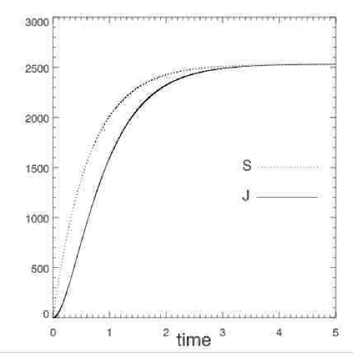
We now use the linear solution (51)-(56) for the two-sided problem with velocity patterns and , respectively in the boundary planes and . Averaging over time-scales bigger than the Alfvénic crossing time, the magnetic field for this solution can be approximated as
| (94) |
and from (87) we can write for the injection energy rate
| (95) |
so that during the linear stage the injection energy rate is always positive.
Chapter 4 Numerical Simulations
Since Parker [67, 72] proposed his nano-flare scenario for coronal heating a number of numerical experiments have been carried out to investigate this idea, with particular emphasis on its possible relationship with the power-law distribution of observed emission events at optical, ultraviolet and x-ray wavelengths of the quiet solar corona. Mikic et al. [56], Longcope & Sudan [53] and Hendrix & Van Hoven [42] carried out simulations using a 3D “straightened out” loop and imposing photospheric shearing given by alternate direction flow patterns. They showed that a complex coronal magnetic field results from the photospheric field line tangling and although the field does not — strictly speaking — evolve through a sequence of static force-free equilibrium states, magnetic energy nonetheless tends to dominate the kinetic energy. In this system, which may be thought of as evolving in a special regime of MHD turbulence, the field is restructured into current sheets elongated along the axial direction.
The numerical investigation of the Parker scenario has been challenging since the beginning. The reasons are the large aspect ratio of a coronal loop, and because the two different time-scales — along the axial direction (the Alfvénic crossing time ) and the perpendicular direction (the non-linear time ), with — together require a large number of grid points. High-resolution simulations are also a necessity when investigating turbulence since this takes place at high Reynolds numbers. Turbulent systems are in fact characterized by a transition to the turbulent state which is not detected at small Reynolds numbers. A limitation of the first simulations carried out during the late 1980s and the early 1990s was their low resolution. While the results of these simulations mostly agreed among themselves, the interpretations that were given did not, and there was not a clear evidence in favor of one of them.
To investigate the turbulent nature of this model with higher resolution, and to carry out long-time simulations necessary to define the statistics of heating events, Einaudi et al. [22] first carried out 2D numerical simulations of incompressible magnetohydrodynamics (MHD) turbulence using a random large scale magnetic forcing function to mimic the forcing exerted in three dimensions by the photosphere. The simulations displayed flux tube behaviour similar to the first 3D simulations, confirmed also in 2D simulations by Dmitruk et al. [16]. These 2D simulations were extended to longer times by Georgoulis et al. [32], and showed for the first time how the magnetically dominated turbulence in the 2D system displays bursts in the dissipation (intermittency) which follow a power law behaviour in total energy, peak dissipation, and duration with indices similar to those determined observationally in X-rays.
Recently Gudiksen & Nordlund [39, 40] have performed numerical simulations of the Parker scenario, modeling a large part of the solar corona with a more realistic geometry. While this approach has advantages when investigating the coronal loop dynamics within its neighboring coronal region, modeling a larger part of the solar corona drastically reduces the number of points occupied by the coronal loops. Thus, these simulations have not been able to shed further light on the physical mechanism responsible for the coronal heating.
In order to further investigate the underlying physical processes at work, we return to the simpler cartesian 3D model, performing numerical simulations with the highest resolution and longest duration to date. In section § 1 we describe the numerical simulations performed with a vortex-like velocity pattern and in § 2 those performed with a sheared velocity pattern. In § 5 we analyze in the framework of anisotropic turbulence theory the results of the simulations.
| Run No. | v, s | n, h | , | ||||
|---|---|---|---|---|---|---|---|
| 1 | v | 200 | n | 800 | 508 | ||
| 2 | v | 200 | n | 400 | 1061 | ||
| 3 | v | 200 | n | 200 | 10 | 2172 | |
| 4 | v | 50 | h | 10 | 196 | ||
| 5 | v | 200 | h | 10 | 453 | ||
| 6 | v | 400 | h | 10 | 77 | ||
| 7 | v | 1000 | h | 10 | 502 | ||
| 8 | s | 200 | n | 800 | 551 | ||
| 9 | s | 200 | n | 400 | 4123 | ||
| 10 | s | 200 | n | 200 | 2356 |
1 Vortex-like Velocity Pattern
In this paragraph we show the results of 3D numerical simulations modeling a coronal layer driven by a forcing velocity pattern constant in time. On the bottom and top planes (respectively and ) we impose two independent velocity forcings, resulting from the linear combination of large-scale eddies. The velocity potential at each boundary is given by
| (1) |
where and , with (corresponding aspect ratio equal to ). The wave number values and used are all those in the range , so that the injection wavenumber is and the corresponding injection scale . and are two sets of random numbers whose values range between 0 and 1
| (2) |
and are independently chosen for the two boundary surfaces.
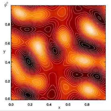

The velocity field follows from equation (4), and the normalization in equation (1) has been chosen so that the rms value of the corresponding velocity is , i.e.
| (3) |
The initial condition is given by the strong uniform axial field specified by the value of the corresponding Alfvénic speed (3). We have performed simulations with different values of .
1 Simulations with
We start showing the results of a numerical simulation performed with , a numerical grid with points and a Reynolds number and . In Figure 1 we show the two boundary velocity patterns (equations (1)) for this simulation which result from a specific random choice of the amplitudes (2). The total duration is roughly axial Alfvénic crossing times (). To remark how challenging these kind of simulations are this simulation has used grid points and time-steps which, using a order runge-kutta, correspond to substeps in which the derivatives have been computed in all the grid points.
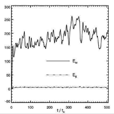
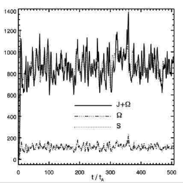
Fig. 2a shows the total magnetic () and kinetic () energies in the loop as a function of time, and Fig. 2b shows both ohmic () and viscous () dissipations and the Poynting flux (the energy that for unit time is injected into the system). All these quantities at first grow following roughly the linear behaviour described by the equations (51)-(56), until time when nonlinearity sets in. The system results magnetically dominated both for energy (magnetic energy is times bigger than kinetic energy ) and dissipation (ohmic dissipation rate is times viscous dissipation ).
In the fully nonlinear regime a statistically steady state is reached, in which the Poynting flux , i.e. the energy which is continuously injected for unit time into the system at the boundaries by the field-line tangling due to the photospheric forcing, balances the energy which is dissipated for unity of time. On the other hand, as previously stated, the Poynting flux, depends not only on the forcing velocity imposed at the boundaries, but also on the value of the magnetic field generated inside the system. This is the reason for which this system must be considered a self-organized system. In fact the balance between Poynting flux and dissipation is reached by letting the magnetic field grow at the opportune value.
In the absence of dynamical evolution, magnetic energy and ohmic dissipation would follow the curves (83)-(84) saturating on a time-scale given by respectively to the values and , well beyond the levels reached in the simulation.

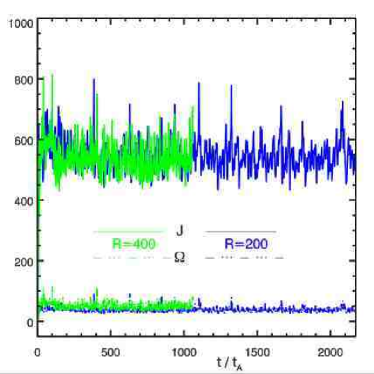
In order to verify the temporal stability of the steady state found in the fully nonlinear regime we have performed other numerical simulations, always with the value for the axial Alfvénic speed, but with lower resolutions and Reynolds numbers to reach longer durations, namely with and with . In this earlier simulations no diffusion along the axial direction was used, i.e. . Time durations are respectively and . In Fig. 3 we show the magnetic and kinetic energies, and the ohmic and viscous dissipation rates as a function of time for these simulations. The results of the previous simulation, which was carried out with a higher resolution, but for a shorter duration, are fully confirmed, and in particular in the nonlinear regime a steady state is reached. In particular the integral quantities, i.e. total energies and dissipation rates, are intermittent in time.
Fig. 3b shows another very interesting result. Ohmic and viscous dissipation rates for the simulations with and roughly overlap. Having a dissipation rate independent of the Reynolds number is a property of turbulent systems where the injection, transfer and dissipation rates are equal (see eq. (105)) and independent of the Reynolds numbers beyond a threshold. The value of the threshold is determined by the diffusion time at the large scale, which must be larger than the nonlinear time-scale. The diffusion time at the scale is , so that at the injection scale for our lowest resolution simulation with the diffusion time is which we can suppose to be beyond the nonlinear timescale. On the other hand both this time-scales depend quadratically on , so that with our lowest resolution we might be just beyond the threshold.
We use hyperdiffusion (see (3)) to eliminate the diffusive effects at the large scales with a dissipativity exponent . In this case the diffusive time at the scale is given by . Numerically we require the diffusion time at the resolution scale , where is the number of grid points, to be the same for both normal and hyperdiffusion, i.e.
| (4) |
So for a grid with 512 points — which has required a Reynolds number with normal diffusion — and a dissipativity , the required hyperdiffusion gives . From equation (73) we find that for a generic dissipativity , including also a diffusive term along the axial direction with Reynolds number , dissipation rate is given by
| (5) |
In general because of the anisotropy of the system , for example in the high-resolution simulation shown in Figure 2 we have even though the values of the Reynolds numbers used are . For normal diffusion the dissipation rate (see equations (73)-(78)) is approximated by , with the ohmic and viscous dissipation rates as defined in (84)-(85).
We have then performed a numerical simulation using hyperdiffusion, with dissipativity , grid points. After a few tests we have used and a Reynolds number for the parallel diffusion . This simulation confirms the results with ordinary diffusion. In Fig. 4 we plot the dissipation rates for the 4 simulations

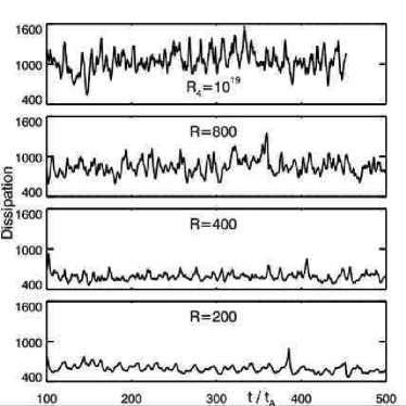
with 3 different Reynolds numbers and hyperdiffusion. The simulations with and do not use parallel diffusion () while those with and hyperdiffusion have . The dissipation rates roughly overlap, in particular those performed with the same numerical methods, i.e. those which implement or not parallel diffusion. We also note that these four simulations do not differ solely for the value of the Reynolds numbers, the number of grid points, and the implementation of parallel diffusion: in each simulation the coefficients that define the spatial shape of the forcing boundary velocities (see eqs. (1)-(2)) are chosen randomly, and are always different. Thus, the four simulations shown in Fig. 4a refer to four different velocity patterns, although all of them have an rms value of (see (3)). The small differences are probably due to this difference more than to the different Reynolds numbers. To further investigate the independence of the dissipation rate on Reynolds numbers it will be necessary to perform these numerical simulations using the same spatial pattern for the boundary velocities and parallel diffusion for all of them. The diffusion time at the large scales has a tremendous increase between and , going from up to , so that the results shown in Figure 4 demonstrate that there is at most a very small variation in the dissipation rates once the diffusion time at the large scales is beyond a threshold.

Figure 4b shows a close-up of the dissipation rates as a function of time at different Reynolds numbers and with hyperdiffusion. At increasing higher Reynolds numbers the function clearly exhibits more fine structures at smaller time-scales. This is a typical feature of a transition to turbulence.
In order to check the validity of these results it is important that the energy equation (85) is numerically well satisfied. Although this equation is not directly integrated by the numerical code, it follows from the equations that are integrated, so that there could be a numerical discrepancy. Indicating with the quantity
| (6) |
which analytically should be equal to , we define as the numerical energy conservation error the absolute value of the normalized quantity . In Figure 5 we plot as a function of time for the numerical simulations just described. The value of is at most 2.5%, with an average of 1.8% for decreasing to 0.15% for , while for and the average errors are respectively 0.9% and 0.4%. Hence the energy conservation equation (85) is numerically very well satisfied.
We now briefly examine the 3D structure of the physical fields. One of the hypothesis of reduced MHD is that during time evolution the orthogonal magnetic field is small compared to the axial component. The orthogonal field component always fluctuates around a value which is roughly the of the the axial field (see Figure 2a) thus verifying this hypothesis. In Fig. 6-7 we show the magnetic field lines, a view from the side and from the top of the computational box respectively. For an improved visualization the box has been rescaled, but it should be noted that the computational box is ten times longer in the axial direction () than in the orthogonal plane. Consequently it can be verified that the magnetic field lines are only slightly bent. In both figures we show the field lines of the orthogonal magnetic field in the mid-plane. The structure of the orthogonal magnetic field is almost invariant in the axial direction and it is structured in magnetic islands. In particular, no boundary layer is present. The lines of the total magnetic field which bend most are those which happen to be at the outskirts of the magnetic islands, where the orthogonal magnetic field is enhanced. Current sheets develop, extended along the axial direction, as shown in Fig. 8-9, and in these thin sheets the energy flux is finally dissipated.
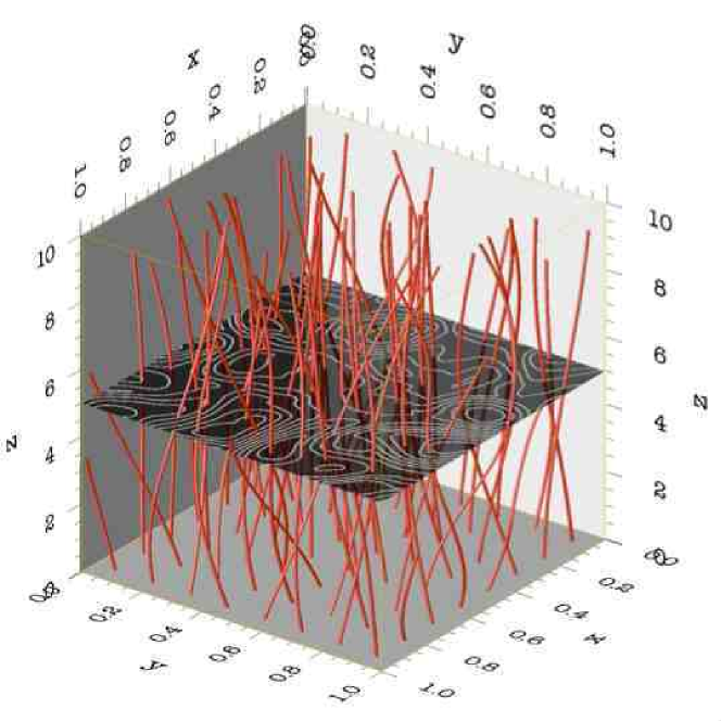

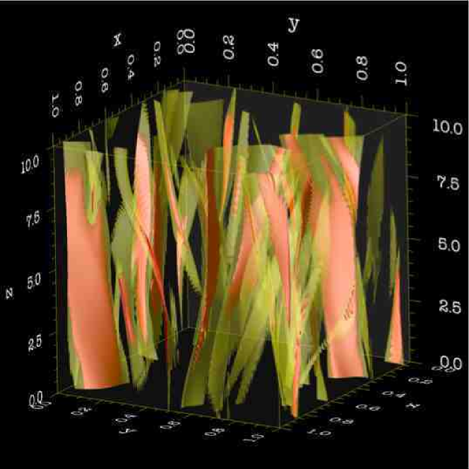

2 Spectral Properties
In this paragraph we discuss the dynamics of our system using its spectral quantities in more detail. We show how the current sheets shown in Figures 8-9 are formed and study the long-time dynamics behaviour.
In turbulence the fundamental physical fields are the Elsässer variables . The analysis of the weak and strong anisotropic turbulence presented in § 4 has been carried out assuming weak velocity-magnetic-field correlation at all scales . This property basically follows from the symmetry in of both the reduced MHD equations (53)-(56) and the boundary conditions used (60)-(61), as shown in § 1, and will be used in all § 5 to perform our nonlinear analysis. The Elsässer variables are associated with the corresponding energies
| (7) |
related to the kinetic and magnetic energies , and to the cross helicity
| (8) |
by
| (9) |
so that the low-correlation of the fields requires . Figure 10a shows this quantity as a function of time for the simulation with , , . The cross helicity fluctuates around zero, with a variation of at most 4% with respect to total energy and an average of 0.54%. Alternatively for a magnetically or kinetically dominated systems, in which one of the two energies exceeds the other, the correlation function is defined as
| (10) |
This quantity is shown as a function of time in Figure 10b. It fluctuates around zero with an average of and a maximum of . Hence the velocity-magnetic-field correlation is very small when the whole computational box is considered. We present a more detailed correlation analysis later in this paragraph.
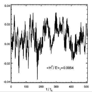
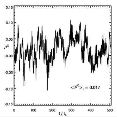
In Figures 11 we show the spectra for run 1. Unless otherwise specified the spectra are one-dimensional, averaged in the axial direction. We define the Fourier transform of a function as
| (11) |
where
The discrete form of Parseval’s theorem gives:
| (12) |
For example considering the energy spectra
| (13) |
Even if is discrete in our case, it is useful to use a continuum formalism through the substitution
| (14) |
In this way we can write the energies as:
| (15) |
and finally integrating along we have , and in the discrete case
| (16) |
In Figure 11a we show the spectrum for run 1.
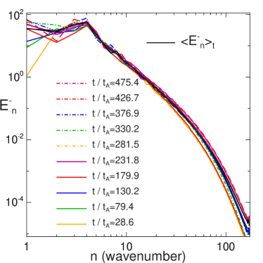

In different colors the spectrum at different times is displayed, while the black line shows the time average of the spectrum performed on a total duration of Alfvénic crossing times. A well-developed spectrum is formed with a peak at , which is the injection scale. This is a clear proof that this system is turbulent and that an energy cascade exists. Figure 11b shows the time averages spectra of the kinetic, magnetic and energies. As expected almost completely overlap, while they are barely distinguishable from the magnetic energy spectrum. The kinetic energy spectrum has noticeably smaller values, and in particular the mode at the injection scale is fixed by the boundary forcing velocity as we show later in this paragraph.
Figure 12 shows a close-up of the time-averaged spectrum. Even if run 1, for which this spectrum has been calculated, used a grid with points and a Reynolds number an inertial range is barely formed and diffusion affects the spectrum at least up to . On the other hand energy is injected at the scale at small wavenumbers, so in this kind of simulation it is very difficult to obtain a well-developed inertial range because very few points are left. Two lines corresponding to energy spectra and are drawn for reference.

In order to study the properties of the inertial range we have used hyperdiffusion, that we will describe in a moment. But now we want to analyze how the current sheets elongated along the axial direction shown in Figures 8-9 are generated.
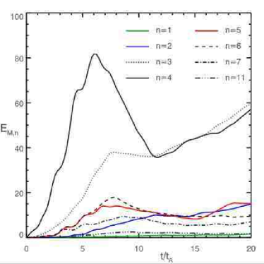
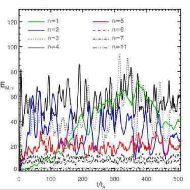
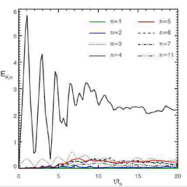


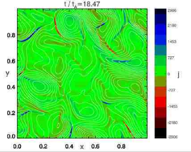
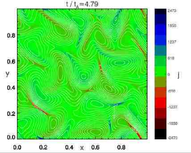


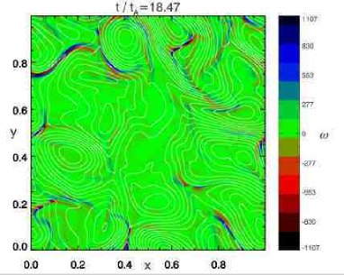
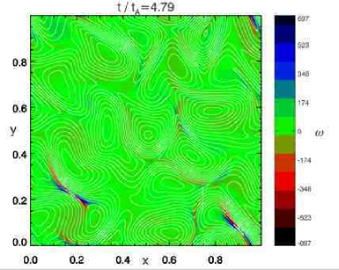
In Figures 13a and 13c we show the first modes and mode for the magnetic and kinetic energy spectra, for the first Alfvénic crossing times . In Figures 14 and 15 we show at selected times, covering the same time-interval, the axial component of the current and vorticity in the midplane . The modes at the injection scale follow the linear dynamics described by equations (51)-(56) until time . In particular the magnetic field and the current at time — i.e. just after time when the two counterpropagating front-waves reach the midplane — are mapping the photospheric velocities as predicted by our linear analys. Figures 1a and 1b show the two photospheric velocity patterns separately, while for comparison with Figure 14a we show the contour of the linear combination in Figure 16a.
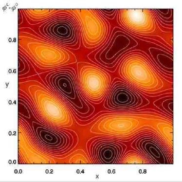

In particular the magnetic energy mode grows roughly quadratically in time, while the kinetic energy mode exhibits a sawtooth structure with a period . The dynamics are described by a cascade towards smaller scales. No instability of any kind is detected. In physical space this cascade corresponds to the formation of small scales which are organized in vortex-current sheets. This picture remains unaltered throughout the rest of the nonlinear stage. Energy is injected at the large scales () by photospheric motions and an energy cascade develops, which transports this energy from the large to the small scales where it is finally dissipated. Figures 14c and 15c show that during the nonlinear stage () the magnetic field exhibits a complex topology and that distorted current sheets are almost always present together with quadrupolar vorticity structures. These current sheets are subsequently subject to tearing, which leads to suppose that the dissipation mechanism is nonlinear magnetic reconnection in a turbulent environment.
An important question is what is the dissipation rate and how much it is influenced by the magnetic reconnection rate. Longcope & Sudan [53] suppose that the reconnection proceeds at a rate independent from the turbulent state of the system, which they completely neglect.
A similar behavior, i.e. microcurrent sheets formed by a turbulent cascade and then subject to tearing, has been detected in decaying 2D turbulence e.g. by Politano et al. [76]. Biskamp & Welter [7] and Biskamp & Schwarz [6] have also studied its influence on dissipation rates. In particular Biskamp & Schwarz [6] have performed the highest resolution 2D MHD simulations finding that the tearing mode occasionally occurs but its influence is rather weak. This is because this reconnection is taking place in a turbulent environment, so that the current sheets dynamics is influenced by the larger-scale dynamics.
Our numerical simulations leads us to suppose that whether or not the reconnection rate is influenced by the turbulent dynamics the tearings happen continuously, so that the energy flux trasported by the cascade is dissipated in many “microbursts”, so that the turbulent energy flux is dissipated in a statistically steady fashion.
In particular, the fact that the spectrum which is developed (see Figure 11) does not show any anomalous structure at smaller scales means that the rate at which energy is dissipated by magnetic reconnection is that at which energy flows along the inertial range. This scenario is reinforced by the fact that when we use hyperdiffusion the spectra that are found are consistent with those expected theoretically for weak anisotropic turbulence, as shown in the following paragraphs.
The only difference detected at longer times is the growth of the and modes for the magnetic energy (see Figures 13b), which show a tendency towards an inverse cascade, even though a complete inverse cascade never fully develops. This is a difference with the corresponding 2D simulations (Einaudi & Velli [21]), where at long times a complete inverse cascade leads to the coalescence of the magnetic islands. The kinetic energy mode at the injection scale fluctuates around an equilibrium value which is the average of its value during the linear regime, and indicates that the dynamics for the modes at do not depart dramatically from the linear behavior (51)-(56).
The inhibition of an inverse cascade is probably due to the stiffness of the magnetic field lines, which are only slightly bent along the axial direction. In fact the magnetic field line tension associated with these field lines inhibits the coalescence of the magnetic islands that form in the orthogonal planes. In Figure 17 we plot the first 4 modes for the magnetic energy with two different values of the axial Alfvénic velocity, respectively and . At the field line tension is smaller than for , and in fact in the first case an inverse cascade is clearly present (Figure 17a) while in the second it is not (Figure 17b).
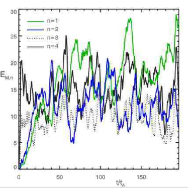
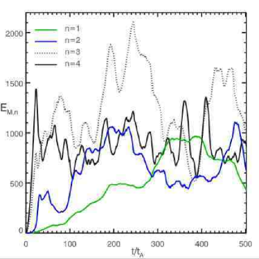
We show in Figure 16b some physical quantities averaged in the planes as a function of the axial direction . Both the magnetic and velocity fields are elongated along the axial direction, as is the current.

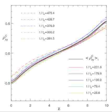
Finally in Figure 18a we show the magnetic helicity density integrated in the planes as a function of at selected times
| (17) |
The figure shows an almost linear behavior of as a function of , confirming the homogeneity of this system in the axial direction. is the axial component of the Poynting vector divided by the Alfvénic velocity (see eq. (89)), i.e.
| (18) |
so that energy is flowing from the boundaries into the computational box at a uniform rate. The energy equation (85) still holds for any slice of the computational box included between two planes so for any two slices of equal volume the rate of injection of energy and the dissipation rate are the same.
The velocity-magnetic field correlations in the planes , which is closely related to the cross helicity density , is defined as
| (19) |
In Figure 18b we show this quantity as a function of at selected times. As expected the velocity and magnetic field are more correlated at the boundaries, where the velocity is imposed as a boundary condition, than in the interior of the computational box.
3 Weak Turbulence Spectra
In order to resolve the inertial range we perfomed a series of high-resolution simulations using hyperdiffusion. The numerical grid was , and the axial Alfvénic velocities are . In Figure 19 we show the time-averaged energy spectrum for these simulations. The time averages have been performed over and respectively.
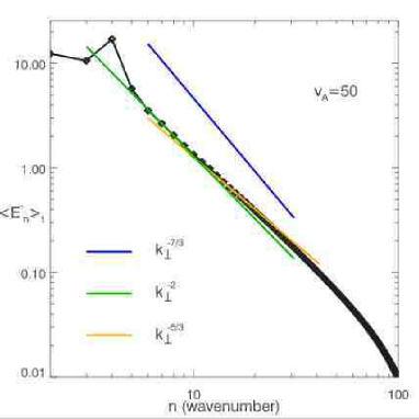
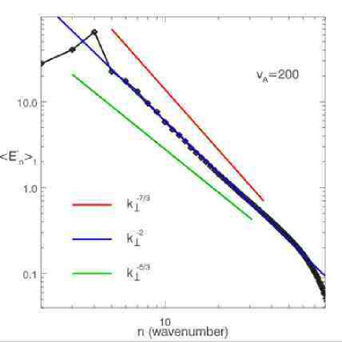
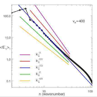

Comparing Figure 19b with Figure 11a we notice that a well-developed inertial range is now present, in contrast to the analogous case with normal diffusion. In the framework of the weak anisotropic turbulence theory that we have briefly surveyed in § 4 the spectral slopes are expected to increase from for strong turbulence, i.e. for turbulent regimes in which the perturbation and the mean field are similar, to steeper exponents as long as we proceed towards weaker regimes of turbulence, i.e. turbulent regimes in which the ratio of the perturbation over the mean field decreases. For weak turbulence the exponents are , i.e. . To distinguish between spectral slopes is usually a difficult task because the differences among them are relatively small. In the case of weak turbulence at increasing the difference between neighboring slopes becomes very small.
Consider Figure 19b, which is the run with the same value of the Alfvénic velocity that we have extensively considered in the previous paragraphs . This is the easiest case: while the line fits well the inertial range, the two neighboring slopes and clearly do not.
A very well known problem with hyperdiffusion is the so-called bottleneck effect (Falkovich [23], Lithwick & Goldreich [52]): the spectrum on scales slightly larger than the dissipation scales becomes flatter (in bilogarithmic scale a small bump appears). The energy, in effect, is backed up and the origin of this reflection is the rapid increase of diffusion at the small scales. Hyperdiffusion virtually removes diffusion from the large scales, but while normal diffusion slowly decreases the diffusion time towards the small scales, hyperdiffusion has a very steep decrease which increases with increasing dissipativity . We have used a mild exponent but the bottleneck effect is present visible, especially in the simulation with (Figure 19c) and (Figure 19d). In Figure 19c the spectrum is steeper than for and the slope that fits better the inertial range is while and certainly do not. Consider now Figure 19d where the spectrum for a simulation with the higher value is shown. Between and , the first slope fits better in the inertial range but and clearly do not fit the inertial range. The case with the lowest value of the Alfvénic velocity shown in Figure 19a. The spectrum shown is an average over Alfvénic crossing times. The slope fails in the inertial range, but and seem to fit the first part and the last part of the inertial range respectively. Actually we could consider if in this case it does develop an inertial range. The slope change which develops around is in a very advanced position towards the small wavenumbers respect to the others simulations to be the bottleneck effect. But we have no objective method to say if this is really a bottleneck effect. There is another possibility. As shown in § 4 all the weak turbulence scalings share the property that at smaller scales the turbulence gets stronger, and Goldreich & Sridhar [34] have proposed the possibility of multiple inertial ranges, where starting, for example, from a slope the system transitions at smaller scales to a stronger regime. If it is already difficult to distinguish numerically one inertial range, it is certainly far more difficult to distinguish among two. Nevertheless in Figure 19a either we have a bottleneck effect or it is this transition, and there is no objective method to decide. It would be certainly interesting to perform a numerical simulation with the same parameters but doubling the resolution.


As already shown, for this system so that . Hence the rms of the fields are also roughly the same, and we now consider the integral quantity
| (20) |
Figure 20a shows the relative ratio as a function of time while Figure 20b show for the four simulations considered in Figure 19. While the value of increases at higher values of , the relative ratio decreases. Hence the results shown in Figures 19-20 show that the our system is described by a weak anisotropic turbulence regime which gets weaker for higher values of the axial Alfvénic velocity .
The physical mechanism by which the system dynamically choses a value for different values of is self-organization. Both this mechanism and its consequences for coronal heating scalings are examined in § 5. We conclude this paragraph showing the dissipation rate as a function of time for the four simulations in Figure 21: the dissipation rate is higher for higher values of .

4 Strong Turbulence and Dissipation
In previous paragraphs we have shown the spectra of many physical quantities always considering the orthogonal variable, and summing over the axial direction.
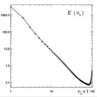

In our simulations we impose non-periodic boundary conditions, along the axial direction , but nevertheless the system results almost periodic, i.e. there are not strong variations along the axial direction. It is then possible to perform a fourier transform of the physical quantities also along the axial direction. As the functions are not strictly periodic we have to expect some “aliasing” at the small scales.
Consider the Fourier expansion (15) for the energies. If instead of summing along we perform the fourier transform we obtain the 2D analogue of the 1D spectra (16), and we can now write
| (21) |
where is the orthogonal wavenumber, and is the axial wavenumber for which also the component does not vanish. From the 2D spectra we easily obtain the 1D orthogonal and axial spectra and summing over the remaining variable, i.e.
| (22) |
In Figure 22 the spectra and at selected values of are shown. Figure 22a shows that already the first few modes have a sharp decrease in their values. Figure 22b shows that at least up to the presence of axial () modes is negligible.
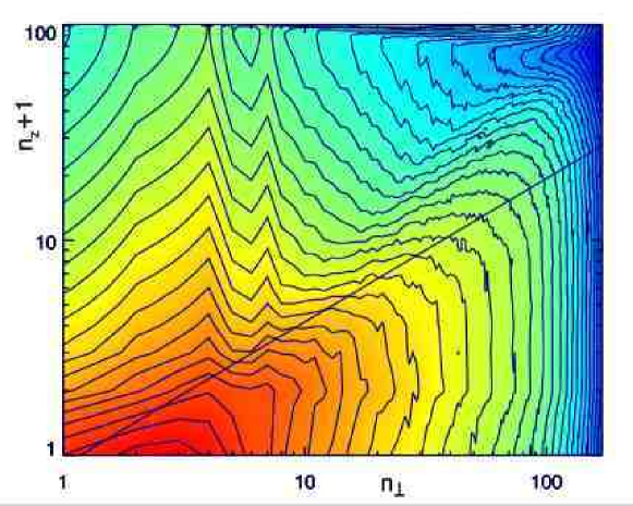
In Figure 23 are shown the contours of the natural logarithm of the 2D spectra. It is clearly shown that at small scales strong turbulence sets in, with the formation of small scales along the axial direction.
2 Sheared Velocity Pattern
In this section we consider the 3D evolution of a coronal layer driven by a time independent forcing pattern. A vanishing photospheric flow is imposed on the bottom plane ()
| (23) |
while on the top plane () the velocity pattern is a stationary photospheric shear flow aligned along the direction
| (24) |
where , and , with an aspect ratio of , i.e. . The initial condition is given by the strong uniform axial field with very small amplitude noise in the perpendicular velocity and magnetic fields. This case is interesting because the growing magnetic field induced in the corona (see equations (81)-(84)) by such motions is an equilibrium field at every instant. In other words, any dynamical evolution beyond the slow increase of magnetic energy with time must be due, at first, to instabilities arising in the system. A similar configuration was used by [44], who developed a semi-analytical quasi self-consistent “turbulent” model of coronal heating. The most interesting result from these simulations is that after the first energetic burst (due to a tearing instability), which releases the energy accumulated during the linear stage, the dynamics are turbulent once the nonlinear stage sets in and are similar for all to those which develop with a vortex-like forcing velocity pattern.
If there were no perturbation at all, at longer times diffusive terms would not be negligible even at large scales and the solution would be modified over diffusive time-scales. While diffusion will only slightly change the shape in of the velocity field, it has a stronger effect on the magnetic field which would otherwise grow linearly in time. We describe briefly such effect. From which the following expressions for the total magnetic energy and ohmic dissipation are obtained:
| (25) |
| (26) |
At first, for a time short compared to the resistive time , both quantities grow quadratically in time while they saturate on the diffusive time-scale. If non-linearity did not set in, the heating rate would saturate at a value that is proportional to the Reynolds number and the square of the axial Alfvénic velocity.
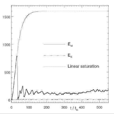
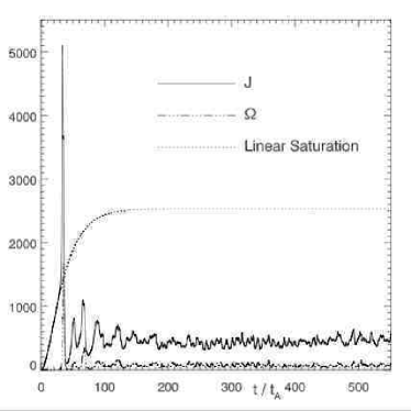
The results of a numerical simulation performed with grid points, a Reynolds number and carried on for roughly axial Alfvénic crossing times () are shown in Figs. 24 and 25. Fig. 24a shows the total magnetic and kinetic energies in the loop as a function of time, Fig. 24b shows ohmic and viscous dissipation, and Fig. 25 shows the total dissipation and the Poynting flux. Magnetic energy grows quadratically at first, reaching a maximum at
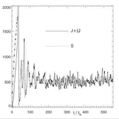
while the kinetic energy is much smaller and remains limited at longer times. In the absence of dynamical evolution, magnetic energy and ohmic dissipation would follow the curves (25)-(26) (as they actually do until when nonlinearity sets in), saturating on the diffusive time-scale , and shown by the dashed lines in Fig. 24. What occurs at is that reconnection begins in the sheared induced field. Given the periodicity of the system, the actual instability is a multiple tearing mode, which grows faster than the classical tearing mode. Until energy is stored in the large-scale magnetic field, while the kinetic energy is only a small fraction of the total energy. This energy is abruptly released in the reconnection event that gives rise to the first big burst in the heating rate that consequently lowers the magnetic energy. After this event a statistically steady state is reached. In this state the Poynting Flux balances the rate of energy dissipation, as shown in Fig. 25. On the other hand, as previously stated, the rate of energy injection into the system, i.e. the Poynting flux, depends on both the forcing velocity imposed at the boundaries and the magnetic field generated inside the system. This is why this system is self-organizing. The balance between Poynting flux input and dissipation rate is reached by letting the magnetic field grow at the “opportune” value, as it is shown in § 5.
Now we examine briefly the 3D structure of the physical fields. One hypothesis of reduced MHD is that during time evolution the orthogonal magnetic field is always small compared to the axial component. After the first big burst, where the ratio of the rms of the orthogonal field over the axial field reaches the , this component always fluctuates around a value which is roughly the . Thus the reduced MHD requirement is satisfied. In Fig. 26-27 we show the magnetic field lines,
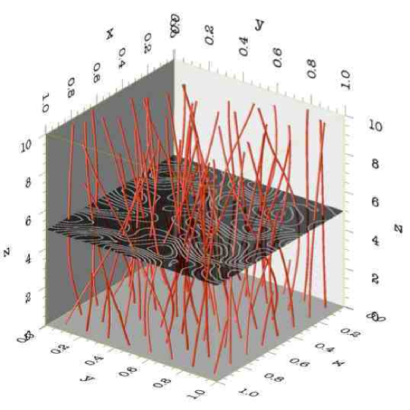

respectively a view from the side and from the top of the computational box. For an improved visualization the box has been rescaled. But it should be noted that the axial length is ten times the orthogonal length of the box. The magnetic field lines are only slightly bent. In both figures we show the field lines of the orthogonal magnetic field in the mid-plane. The structure of the orthogonal magnetic field is almost invariant in the axial direction and it is structured in magnetic islands. In particular no boundary layer is present. The field lines of the total magnetic field which bend more are those which happen to be inside the magnetic islands where the orthogonal magnetic field is enhanced. The magnetic island structure for the magnetic field gives rise to current sheets elongated along the axial direction, as shown in Fig. 28-29, where the energy flux is finally dissipated.
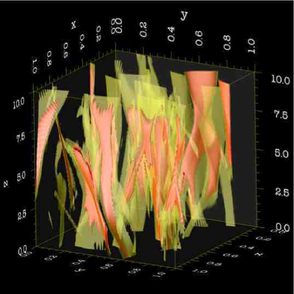
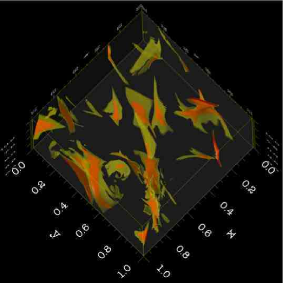
We have also performed other numerical simulations with different Reynolds numbers and spatial resolutions. In Figs. 30 we show the
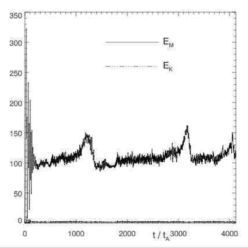
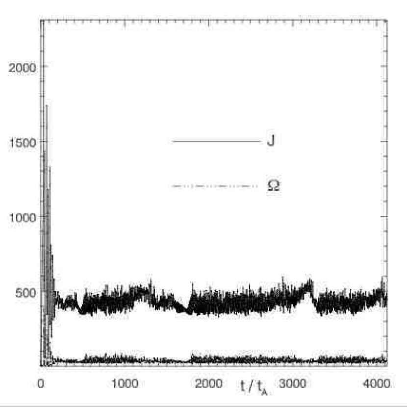
results of a very long simulation with grid points, a Reynolds number and carried on for more than . The results of the previous simulation, which was carried out with a higher resolution, but for a shorter duration, are fully confirmed. In particular the longer interval allows us to confirm that after the first reconnection event a steady state is finally established.
We have another very interesting result. In Fig. 31 we plot ohmic dissipation for 3 numerical simulations
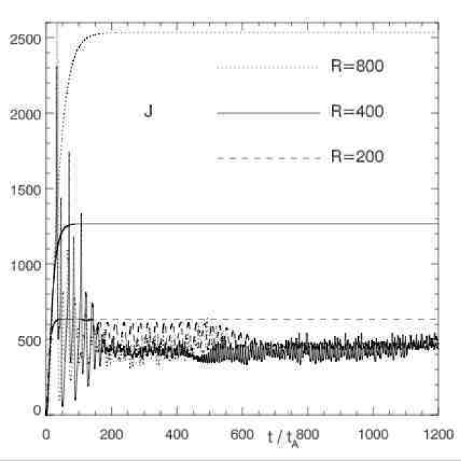
carried out with 3 different Reynolds numbers, and . As the Figure clearly shows they overlap. This supports our hypothesis that the dynamics are turbulent and that the dissipation is independent of the Reynolds number. In Fig. 32 a close-up of

the dissipation functions with time at different Reynolds number is shown. A clear transition to turbulence is present, the appearance of progressively more fine structure as the Reynolds number increases. Note that the dissipation is independent of the Reynolds number only beyond a threshold below which diffusion is important even at large scales, and consequently most of the energy is diffusively lost from the field at large scales before it can reach the small scales. In particular in the case of the sheared forcing considered in this simulation, if we decrease the Reynolds number below the diffusive time is so short that no instability can grow, and the system follows the linear saturation curves, showing no sign at all of nonlinear dynamics.
Chapter 5 Nonlinear Analysis: Self-Organized Anisotropic Turbulence
As already mentioned in § 3 one of the main original results of this work is the connection between the heating of closed magnetic structures in the solar corona and anisotropic turbulence. In an environment threaded by a strong axial magnetic field, Alfvén wave packets traveling in opposite directions are naturally present. In coronal loops they are excited by photospheric motions on scales of the order of the cross-length of a granule (). Their “collisions” give rise to a turbulent cascade which transfers energy from the large to the small scales, where it is finally dissipated, i.e. converted to heat and particle acceleration. Current sheets elongated in the axial direction are a feature found in most of the previous numerical simulations carried out to model a coronal loop. There have been many explanations about the formation of these structures. In the framework of anisotropic turbulence, these structures spontaneously develop. In fact the cascade of energy mainly takes place in the orthogonal planes while it is strongly reduced in the axial direction, so the turbulent transfer of energy to smaller perpendicular scales results in sheet-like structures elongated in the direction of the main field.
In this section we analyze our system using the theory of anisotropic turbulence, of which we have given a review of the current state in § 4. As it usually happens in most of turbulence theory, the system studied is modeled as a three-dimensional three-periodic one. Periodicity leads to the cancellation of all the flux terms at the boundary surfaces. In a realistic model of a coronal loop, the axial direction cannot be modeled as periodic, and in particular the energy flux originating from the photospheric surfaces is just the source of energy for the system, which of course cannot be neglected. The inclusion of the energy flux terms at the boundaries gives to the system the property to be self-organized. In fact while the amplitude of the perturbations is usually imposed to be “small” on some physical ground, in a coronal loop it is the system itself that sets this amplitude, as described in the following sections.
1 Self-Organization and Scalings
In a turbulent system energy is injected into the system at the rate at the scale , it is subsequently scattered along the inertial range with the transfer rate , and finally dissipated at the dissipation scale at the rate . For balance all these fluxes must be equal
| (1) |
This equality still holds approximately when, as in our case, changes in time, because the more rapid dynamics at the small scales in the inertial and dissipation ranges adjust the spectrum rapidly compared to the slower dynamics of the large scales. In our case the value of is given by (93), the integral of the Poynting flux at the boundaries, and the transfer rate is given by the anisotropic turbulence theory (see § 4). Both and depend on the value of the internal fields, so that the balance equality (1) fixes their value.
In our numerical simulations the injection scale is , that we approximate to in the following calculations. Elsässer variables are the fundamental variables in turbulence theory. The nonlinear terms in the equations of reduced MHD (53)-(56) are symmetric in the exchange of these two variables
| (2) |
while the linear terms simply describe a wave propagation in opposite directions for the two fields . Furthermore, in our case, the boundary conditions (60)-(61), that we rewrite for convenience,
| (3) |
| (4) |
are also symmetric in the exchange. In this way the rms values of are approximately equal at all scales, i.e. indicating with the rms value of the field at the scale
| (5) |
This is equivalent to say that we expect the cross helicity
| (6) |
to vanish. This is also confirmed by our linear analysis (see § 3) which has shown that the magnetic field is noticeably bigger than the velocity field, and by our numerical simulations (see Figure 10). As the velocity field is smaller than the magnetic field we can also approximate in the Poynting flux integral (93) the magnetic field at the injection scale with the Elsässer variable, i.e. , so that identifying the injections energy rate with S we have
| (7) |
The energy injection rate is directly proportional to the rms of the Elsässer fields at the injection scale . The velocity forcing at the boundaries injects energy with the rate (7) at the scale smaller than the axial lenght , developing a perturbation .
The strongly reduced cascade along the axial direction implies that the wave packets have size of the order along this direction, while in the ortogonal plane a turbulent cascade with the characteristics described in § 4 takes place. We now apply the theory of anisotropic turbulence (see § 4) to have the value of the transfer energy rate .
We start from the anisotropic version of the Iroshnikov-Kraichnan theory described in equations (134)-(142) and characterized by the orthogonal spectrum . Indicating with the eddy turn-over time and with the Alfvénic crossing time, the number of collisions for the fractional perturbation to build up to order unity is
| (8) |
so that the energy transfer time is given by
| (9) |
and the energy flux for unitary volume is given by
| (10) |
Usually the value of the spectral flux or equivalently of the perturbation at the large scale are fixed to a “small” value on some physical ground. In our model this value is self-consistently established. Multiplying equation (10) by the volume in order to have the total flux, and considering the injection scale we have
| (11) |
This is the flux of energy that leaves the injection scale towards the small scales, and that is supposed to have a constant value along all the inertial range. Equations (7) and (11) show that the system is self-organized. In fact both and depend by , the rms value of the Elsässer variables at the injection scale , so that the internal dynamics depends by the injection of energy and the injection of energy depends by the internal dynamics. As shown in
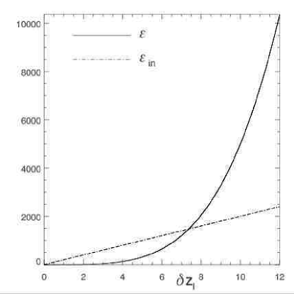
Figure 1 the two fluxes satisfy the equality condition (1) only for the value
| (12) |
For a value of the perturbation smaller than (12) the injection flux is higher than the dissipation one, so that the pertubation grows toward the equilibrium value. On the opposite for higher values than (12) the dissipation flux is higher than the injection one, decreasing the value of the perturbation . The system is dynamic and turbulent so that we will have fluctuations around this equilibrium value.
Substituting the equilibrium value (12) in (11) or equivalenty (7), we obtain the average spectral flux
| (13) |
As previously said (see (1)) the injection, transfer and dissipation rates balance, so that equation (13) holds for all of them, in particular for the dissipation rate that is also the heating rate, i.e. the rate at which energy is converted to heat and particle acceleration at the dissipation scale .
As shown in § 4, anisotropic turbulence is characterize by different regimes to which correspond different slopes of the spectrum . The relative amplitude of the perturbation relatively to the axial Alfvénic velocity indicates in which regime is the system. In particular at smaller values of this ratio correspond higher slopes in the energy spectrum. In our case from equation (12) we have that
| (14) |
This means that changing the ratio , the relative amplitude of the perturbations changes, and we move among different regimes of anisotropic turbulence, in particular increasing the value of the axial magnetic field increaseas and the ratio (14) decreases.
Previous results can be generalized to the other scalings for anisotropic turbulence described in § 4. The different scalings are characterized by the different number of collisions that a wave packet must suffer for the perturbation to build up to order unity. Introducing the parameter we can write
| (15) |
where and so that for the energy transfer time we have
| (16) |
and finally for the transfer energy rate
| (17) |
Flux (17) is supposed to be constant along the inertial range, so that we can consider its value at the injection scale :
| (18) |
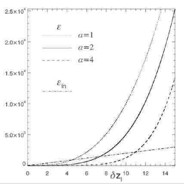

The injection energy rate is always given by (7). For we have the anisotropic Kolmogorov spectrum , while for we have the anisotropic IK spectrum and for the SG94 spectrum based on 4-waves resonant interactions . In Figure 2a energy fluxes (18), for different values of the parameter , and (7) are plotted as a function of the perturbation . There is always an equilibrium value where the two fluxes are equal, while for a higher value of the perturbation the transfer rate is bigger than the injection rate and for a lower value of the perturbation the transfer rate is smaller than the injection rate. From (18) and (7) we have that the equilibrium value for is given by
| (19) |
and substituting this value in (18) or (7) we obtain the coronal heating scalings
| (20) |
which are plotted, for different values of the parameter , in Figure 2b. To higher values of the parameter correspond higher heating rates.
The regime of anisotropic turbulence is determined by the ratio , which from (19) is given by
| (21) |
As , the property that to higher values of the Alfvénic velocity corresponds a smaller relative perturbations is preserved, whatever the anisotropic turbulent regime is. This means that in general none of the different scalings (20) corresponding to different values of is valid for the whole range of the possible values of . In fact, starting form a low value of strong anisotropic turbulence will develop, corresponding to a spectral index and a coronal heating rate (20) with and . Increasing the system transitions to an anisotropic IK regime characterized by , the spectral slope and . Increasing still the value of the Alfvénic velocity will cause the system to transition in the regime characterized by , the spectral slope and . So that the scalings for the coronal heating as a function of the Alfvénic velocity , is characterized by regions with increasing slopes in correspondence of increasing values of , each region characterized by the scaling (20) with an increasing value of the parameter .
2 Timescales
From equations (15)-(20) we can derive the values of the eddy turn-over time , the energy transfer rate (16) and the number of collisions at the scale (15). After a few algebraic calculations we have
| (22) |
and
| (23) |
where is the crossing time used as characteristic time to render the reduced MHD equations dimensionless, and is the axial Alfvénic crossing time. For our system
| (24) |
so that . The number of collisions has always the property to decrease at small scales, leading to a stronger turbulent regime. Except for where correctly the energy transfer time and the eddy turn-over time are equal, for all the others regime ()
| (25) |
the energy transfer time is bigger than the eddy turn-over time, which is a characteristic of the Alfvén effect at the basis of the anisotropic turbulence theory.
An interesting quantity is the energy transfer time at the large scales which can be identified with the nonlinear timescale , i.e.
| (26) |
which in dimensionless units is .
The nonlinear time is also the time at which the linear stage transitions into the nonlinear stage. This results from the following calculations. The linear stage dynamics is described in § 3, and in particular we use the solution (51)-(56) for the two-sided problem with velocity patterns and , respectively in the boundary planes and . Averaging over time-scales bigger than the Alfvénic crossing time, the magnetic field for this solution can be approximated as
| (27) |
Since during the linear stage the magnetic field has only large-scale components, we can approximate
| (28) |
and from (87) we can write for the injection energy rate
| (29) |
From this equation we can also note the important property that during the linear stage the injection energy rate is always positive. The energy flux along the inertial range is the rate at which the energy is leaving the large scales towards the small scales, and substituting the value (28) for in (18) we have for the energy transfer rate

| (30) |
Since the injection of energy is higher than the dissipation, until time
| (31) |
where they become equal, and of course where the linear regime is no longer valid.
Chapter 6 Conclusions and Discussion
In this thesis I have presented the results of the numerical and analytical investigations of a reduced MHD realization of the Parker Scenario for coronal heating. This is the 3D extension of earlier 2D investigations by Einaudi, Velli, Politano & Pouquet [22], Einaudi & Velli [21], Georgoulis, Velli & Einaudi [32].
Parker [68], [69], [70], [71] was the first to propose that the X-ray corona is heated by dissipation at the many small current sheets forming in a coronal loop as a consequence of the continuous shuffling and intermixing of the footpoints of the field by the photospheric convection. Analogous to the linear analysis performed in § 3 the magnetic field results from a continuous mapping of the footpoints velocity pattern. He supposed that the magnetic field spontaneously produces tangential discontinuities (current sheets) which become increasingly severe with continued winding and interweaving, eventually producing intense magnetic dissipation by magnetic reconnection. This dissipation is characterized by bursts of rapid reconnection that he named “nanoflares”.
This picture is, however, “static” (as opposed to “dynamic”) because the magnetic field-lines are assumed to result from “quasi-static” displacements of the magnetic fields, and the current sheets are a consequence of the displacement of two neighboring field lines in opposite directions. The system does not show any dynamics, the field lines are passively bent by the photospheric motions, and the formation of the current sheets is almost “geometric”.
The first numerical simulation of the Parker Scenario was been performed in 1989 by Mikic, Schnack & Van Hoven [56], who found that current sheets formed, extended in the axial direction. Similar results were found later by Longcope & Sudan [53] and Hendrix & Van Hoven [42] respectively in 1994 and 1996. The original “static” picture has remained the basis of all studies of the Parker Scenario. In particular, Longcope & Sudan [53] derive a scaling law for coronal heating as if this were due to magnetic reconnection of the large-scale field. Hendrix & Van Hoven [42] also found current sheets extended in the axial direction and an inertial range but still thought that magnetic reconnection is responsible for the turbulence, describing it as “spontaneous unstably driven MHD turbulence” [42]. All these simulations used a relatively low resolution, i.e. a small Reynolds number, and could not observe the full turbulent dynamics.
In this work, using high-resolution simulations, we have conclusively shown that the transfer of energy from the large-scales, where energy is continuously injected by photospheric motions, towards the small scales is due to weak anisotropic turbulence. The small scale organizes into vortex-current sheets (a common feature in MHD turbulence) that result from the non-linear cascade. They may eventually break up due to tearing and magnetic reconnection, but are certainly not primarily generated by a reconnection instability due to the large-scale field. Magnetic reconnection of these cascade-produced current sheets certainly plays a role in the dissipation of energy, i.e. in the conversion of the energy flowing along the inertial range into heat and particle acceleration. In any case the dissipation mechanism, which acts at the small scales, cannot be properly investigated with a fluid model because these are very well known to break at small scales and/or high frequencies. Thus, a kinetic investigation is appropriate.
In my view the difficulty in realizing that the dynamics of a coronal loop is turbulent has been partially because a theory of weak turbulence for an MHD system embedded in a strong axial field has only recently been developed, mainly due to Sridhar & Goldreich (1994) [86] who studied this mechanism for the first time and find the spectrum. The debate followed with the remarks of Montgomery & Matthaeus (1995) [60], while Goldreich & Sridhar (1997) [34] found for the first time the spectrum and propose a multiple inertial range. Ng & Bhattacharjee (1997) [62], and Galtier et al. (2000,2002) [30, 31] then develop a kinetic model.
Weak turbulence has been barely investigated numerically. Cho & Vishniac (2000), Maron & Goldreich (2001) and Müller & Biskamp (2000) have performed three-dimensional simulations of strong MHD turbulence stretching the abilities of the fastest supercomputers. Simulations of weak turbulence are more difficult because each wavepacket must interact many times with oppositely directed ones before it cascades; by contrast, a wavepacket cascades in strong MHD turbulence in the time it takes to cross a single oppositely directed wavepacket.
Our investigations show that:
-
•
The dynamics are described by weak turbulence. Because the system is embedded in a strong axial field the cascade takes place in the orthogonal planes and is strongly inhibited in the axial direction. Wave-packets are “long-lived” and they need to collide many times before transferring energy to smaller scales.
-
•
The spectral slopes are in agreement with those derived from weak turbulence theory. The energy spectra slopes change from for to for . The slope increase takes place while the rms of the orthogonal fields grows in absolute magnitude but its relative magnitude decreases, in accordance with the theory.
-
•
Small-scales structures do not homogeneously distribute in the planes but organize in vortex-current sheets extended in the axial direction where the energy flowing along the inertial range finally dissipates.
-
•
In the framework of weak turbulence these extended structures are naturally formed because the cascade in the axial direction is strongly inhibited. Hence no boundary layer is present. On the other hand in a real coronal loop a boundary layer, the transition region, is present. This result implies that it has others physical origins.
-
•
Since the rate of injection of energy by photospheric motion depends not only on the photospheric velocity but also on the fields that develop into the computational box the system is self-organized. We have shown that the rms amplitude of the magnetic field at the large scales, which would grow linearly in time were it not for the non-linear dynamics, is fixed by the equality of the injection energy rate and the rate at which energy flows from the large scales towards the small scales, which is the transfer energy rate along the inertial range .
-
•
The weak turbulence and the self-organization of the system lead to the new coronal heating scalings (20)
(1) where is the rate of energy flowing from the injection scale towards the small scales along the inertial range where finally dissipates. We have shown in § 1 that there is not a single scaling law, but that the dissipation rate depends on the regime of weak turbulence in which the system relaxes, described in the previous equation by the parameter . We have also shown that to higher values of the Alfvénic velocity corresponds weaker turbulent regimes characterized by a higher value of the parameter and thus leading to a more efficient heating rate.
The system we have studied is a rather schematic model of a coronal loop. In particular we have not considered density or magnetic field variations along the axis of the loop. The least realistic assumptions are the boundaries, at which the energy is injected and hence are critical to model. Our model should be considered to apply to the extended central part of a loop, beyond the transition region, where the hypothesis of homogeneity along the axial direction is justified.
The first step towards a more complex model is to consider a more complex forcing velocity. A compressible code gives the possibility to use more realistic photospheric motions, including at the same time compressible effects into the dynamics. The first compressible simulations using an incompressible forcing velocity pattern (Dahlburg [13]) confirm the picture shown in this thesis. A future model for the numerical and theoretical investigation of a coronal loop dynamics should consider the underlying regions from the photosphere up to the transition region and of their mutual influences.
Part 1 Slow Solar Wind
Chapter 7 The Slow Solar Wind Acceleration
During the first part of my Ph.D. I have completed a work about the acceleration of the slow solar wind, which I had previously started for my “Laurea” thesis. This work has led to the publication of a paper (Rappazzo et al. [79]) which is reproduced in the Appendix. In the following a brief review is given.
Although the association between the slow solar wind and the streamer belt (e.g. Gosling et al. [35]) and between the fast wind and the polar coronal holes is broadly recognized, the mechanism which leads to the slow and fast acceleration is still a matter of debate. Einaudi et al. [21] developed an MHD model, with a current sheet embedded in a broader wake flow, that accounts for some of the typical features observed in the slow component of the solar wind. Reconnection of the magnetic field occurs at the current sheet and, in the non-linear regime, when the equilibrium magnetic field is substantially modified, a Kelvin-Helmoltz instability develops, leading to the acceleration of density enhanced magnetic islands.
The solar streamer belt is a structure consisting of a magnetic configuration centered on the current sheet, which extends above the cusp of a coronal helmet. The region underlying the cusp is made up of closed magnetic structures, with the cusp representing the point where separatrices between closed and open field lines intersect. Further from the Sun, at solar minimum, the streamer belt around the equator appears as a laminar configuration consisting of a thick plasma sheet with a density about 1 order of magnitude higher than the surrounding plasma, in which much narrower and complex structures are embedded. As a first approximation, moving from the center of the streamer in polar directions at radii greater than the radius of the cusp, the radial component of the magnetic field increases from zero, having opposite values on the two sides of the current sheet. As far as the flow distribution is concerned, the fast solar wind originates from the unipolar regions outside the streamer belt, while the slowest flows are located at the center of the sheet.
One of the most interesting findings of the LASCO instrument onboard the Solar and Heliospheric Observatory (SOHO) spacecraft has been the observation of a continuous outflow of material in the solar streamer belt. An analysis performed using a difference image technique (Sheeley et al. [85], Wang et al. [94]) has revealed the presence of plasma density enhancements, called blobs , accelerating away from the Sun. These plasmoids are seen to originate just beyond the cusps of helmet streamers as radially elongated structures a few percent denser than the surrounding plasma sheet, of approximately 1 Solar Radius () in length and in width. They are observed to accelerate radially outward maintaining constant angular spans at a nearly constant acceleration up to the velocity of 200-450 km/s, in the spatial region between about 5 and . It has been inferred that the blobs are tracers of the slow wind, being carried out by the ambient plasma flow.
In my work [79] I have included in the previous model (Einaudi et al. [21]) spherical geometry effects, taking into account either the radial divergence of the magnetic field lines and the average expansion suffered by a parcel of plasma propagating outward, using the Expanding Box Model (EBM), and the diamagnetic force due to the overall magnetic field radial gradients, the so-called melon-seed force. I have found that the values of the acceleration and density contrasts can be in good agreement with LASCO observations, provided the spherical divergence of the magnetic lines starts beyond a critical distance from the Sun and the initial stage of the formation and acceleration of the plasmoid is due to the cartesian evolution of MHD instabilities. This result provides a constraint on the topology of the magnetic field in the coronal streamer, which observationally is unknown.
Appendix
In this appendix we have included the paper A. F. Rappazzo, M. Velli, G. Einaudi and R. B. Dahlburg “Diamagnetic and Expansion Effects on the Observable Properties of the Slow Solar Wind in a Coronal Streamer”, ApJ, 2005, volume 633, part 1, pages 474-488 http://dx.doi.org/10.1086/431916.
References
- [1] H. Alfvén. Mon. Not. Roy. Astron. Soc., 107:211, 1947.
- [2] Y. Aoyama and J. Nakano. RS/6000 SP: Practical MPI Programming. IBM-ITSO, Austin, 1999.
- [3] M. A. Berger and G. B. Field. J. Fluid Mech., 147:133, 1984.
- [4] L. Biermann. Naturwissenschaften, 33:118, 1946.
- [5] D. Biskamp. Magnetohydrodynamic Turbulence. Cambridge University Press, Cambridge, 2003.
- [6] D. Biskamp and E. Schwarz. Phys. Plasmas, 8:3282, 2001.
- [7] D. Biskamp and H. Welter. Phys. Fluids, 1:1964, 1989.
- [8] C. Canuto, M. Y. Hussaini, and A. Quarteroni. Spectral methods in fluid dynamics. Springer, New York, 1988.
- [9] S. Chandrasekhar. Hydrodynamic and Hydromagnetic Stability,. Cambridge University Press, Cambridge, 1961.
- [10] A. Cho, J. Lazarian and E. T. Vishniac. ApJ, 564:291, 2002.
- [11] J. Cho and E. T. Vishniac. ApJ, 539:273, 2000.
- [12] R. B. Dahlburg. Phys. Plasmas, 5:133, 1998.
- [13] R. B. Dahlburg. Private communication, 2006.
- [14] R. B. Dahlburg, P. Boncinelli, and G. Einaudi. Phys. Plasmas, 5:79, 1998.
- [15] J. M. Davila. ApJ, 317:514, 1987.
- [16] P. Dmitruk, D. O. Gómez, and E. E. DeLuca. ApJ, 505:974, 1998.
- [17] P. Dmitruk, D. O. Gómez, and W. H. Matthaeus. Phys. Plasmas, 10:3584, 2003.
- [18] B. R. Durney, D. S. D. Young, and I. W. Roxburgh. Solar Phys., 145(2):207, 1993.
- [19] G. Einaudi, P. Boncinelli, R. B. Dahlburg, and J. T. Karpen. J. Geophys. Res., 104:521, 1999.
- [20] G. Einaudi, S. Chibbaro, R. B. Dahlburg, and M. Velli. ApJ, 547:1167, 2001.
- [21] G. Einaudi and M. Velli. Phys. of Plasmas, 6:4146, 1999.
- [22] G. Einaudi, M. Velli, H. Politano, and A. Pouquet. ApJ, 457:L113, 1996.
- [23] G. Falkovich. Phys. Fluids, 6:1411, 1994.
- [24] A. Ferrari and E. Trussoni. MNRAS, 205:515, 1983.
- [25] J. M. Finn and T. M. Antonsen. Comments Plasma Phys. Controlled Fusion, 26:111, 1985.
- [26] Message Passing Interface Forum. MPI: A message-passing interface standard. International Journal of Supercomputer Applications, 8(3/4):165, 1994.
- [27] Message Passing Interface Forum. MPI-2: A message-passing interface standard. International Journal of High Performance Computing Applications, 12(1-2):1, 1998.
- [28] M. Frigo and S. G. Johnson. The design and implementation of FFTW3. Proceedings of the IEEE, 93 (2):216, 2005.
- [29] U. Frisch. Turbulence. Cambridge University Press, Cambridge, 1995.
- [30] S. Galtier, S. V. Nazarenko, A. C. Newell, and A. Pouquet. J. Plasma Phys., 63:447, 2000.
- [31] S. Galtier, S. V. Nazarenko, A. C. Newell, and A. Pouquet. ApJ, L49:564, 2002.
- [32] M. K. Georgoulis, M. Velli, and G. Einaudi. ApJ, 497:957, 1998.
- [33] P. Goldreich and S. Sridhar. ApJ, 438:763, 1995.
- [34] P. Goldreich and S. Sridhar. ApJ, 485:680, 1997.
- [35] J.T. Gosling, G. Borrini, J.R. Asbridge, S.J. Bame, W. C. Feldman, and R.T. Hansen. J. Geophys. Res., 86:5438, 1981.
- [36] R. Grappin and M. Velli. J. Geophys. Res., 101:425, 1996.
- [37] R. Grappin, M. Velli, and A. Mangeney. Phys. Rev. Lett., 70:2190, 1993.
- [38] W. Gropp, E. Lusk, and A. Skjellum. Using MPI: Portable Parallel Programming with the Message-Passing Interface. The MIT Press, Cambridge, 1999.
- [39] B. V. Gudiksen and Å. Nordlund. ApJ, 572:L113, 2002.
- [40] B. V. Gudiksen and Å. Nordlund. ApJ, 618:1020, 2005.
- [41] M. Guhathakurta, T. E. Holzer, and R. M. MacQueen. ApJ, 458:817, 1996.
- [42] D. L. Hendrix and G. Van Hoven. ApJ, 467:887, 1996.
- [43] J. Heyvaerts and E. R. Priest. A&A, 117:220, 1983.
- [44] J. Heyvaerts and E. R. Priest. ApJ, 390:297, 1992.
- [45] P. S. Iroshnikov. Sov. Astron., 7:566, 1964.
- [46] B. B. Kadomtsev and O. P. Pogutse. Sov. J. Plasma Phys., 1:389, 1974.
- [47] A. N. Kolmogorov. Dokl. Akad. Nauk. SSSR, 30:299, 1941.
- [48] R. H. Kraichnan. Phys. Fluids, 8:1385, 1965.
- [49] A. Lazarian and E. T. Vishniac. ApJ, 517:700, 1999.
- [50] S. K. Lele. J. Comput. Phys., 103:16, 1992.
- [51] H. Lin. ApJ, 446:421, 1995.
- [52] Y. Lithwick and P. Goldreich. ApJ, 528:1220, 2003.
- [53] D. W. Longcope and R. N. Sudan. ApJ, 437:491, 1994.
- [54] J. Maron and P. Goldreich. ApJ, 554:1175, 2001.
- [55] M. Meneguzzi and A. Pouquet. J. Fluid Mech., 205:297, 1989.
- [56] Z. Mikic, D. D. Schnack, and G. Van Hoven. ApJ, 338:1148, 1989.
- [57] L. J. Milano, D. O. Gómez, and P. C. H. Martens. ApJ, 490:442, 1997.
- [58] D. Montgomery. Phys. Scripta, T2/1:83, 1982.
- [59] D. Montgomery. Lecture Notes on Turbulence, Eds. J. R. Herring & J. C. McWilliams, World Scientific:132, 1987.
- [60] D. Montgomery and W. H. Matthaeus. ApJ, 447:706, 1995.
- [61] W.-C. Müller and D. Biskamp. Phys. Rev. Lett., 84:475, 2000.
- [62] C. S. Ng and A. Bhattacharjee. Phys. of Plasmas, 4:605, 1997.
- [63] A. M. Obukhov. Izv. Akad. Nauk. SSSR, Ser. Geofiz., 4-5:453, 1941.
- [64] D. E. Osterbrook. ApJ, 134:347, 1961.
- [65] E. N. Parker. Phys. Rev., 96:1686, 1954.
- [66] E. N. Parker. ApJS, 3:51, 1957.
- [67] E. N. Parker. ApJ, 174:499, 1972.
- [68] E. N. Parker. Cosmical Magnetic Fields. Clarendon Press, Oxford, 1979.
- [69] E. N. Parker. ApJ, 264:642, 1983.
- [70] E. N. Parker. Geophys. Ap. Fluid Dyn., 35:277, 1986.
- [71] E. N. Parker. ApJ, 330:474, 1988.
- [72] E. N. Parker. Rev. Mod. Astr., 4:1, 1991.
- [73] E. N. Parker. ApJ, 372:719, 1991.
- [74] K. Petrovay and G. Szakály. A&A, 274:543, 1993.
- [75] G. W. Pneuman and P. J. Cargill. ApJ, 288:653, 1985.
- [76] H. Politano, A. Pouquet, and P. L. Sulem. Phys. Fluids, 1:2330, 1989.
- [77] W. H. Press, S. A. Teukolsky, W. T. Vetterling, and B. P. Flannery. Numerical Recipes. Cambridge University Press, Cambridge, 1992.
- [78] E. R. Priest. Solar Magnetohydrodynamics. Reidel, Dordrecht, 1982.
- [79] A. F. Rappazzo, M. Velli, G. Einaudi, and R. B. Dahlburg. ApJ, 633:474, 2005.
- [80] T. P. Ray. MNRAS, 198:617, 1982.
- [81] P.L. Roe and D.S. Balsara. SIAM J. Appl. Math., 56:57, 1996.
- [82] J. M. Schmidt and P. J. Cargill. J. Geophys. Res., 105:10455, 2000.
- [83] M. Schwartzschild. ApJ, 107:1, 1948.
- [84] J. V. Shebalin, W. H. Matthaeus, and D. Montgomery. J. Plasma Phys., 29:525, 1983.
- [85] N. R. Sheeley et al. ApJ, 484:472, 1997.
- [86] S. Sridhar and P. Goldreich. ApJ, 432:612, 1994.
- [87] R. F. Stein and J. Leibacher. Ann. Rev. Astr. Ap., 12:407, 1974.
- [88] H. R. Strauss. Phys. Fluids, 19:134, 1976.
- [89] T. Stribling, D. A. Roberts, and M. L. Goldstein. J. Geophys. Res., 101:27603, 1996.
- [90] P. A. Sturrock and Y. Uchida. ApJ, 246:331, 1981.
- [91] K. W. Thompson. J. Comput. Phys., 68:1, 1987.
- [92] K. W. Thompson. J. Comput. Phys., 89:439, 1990.
- [93] T. X. Vanajakshi, K. W. Thompson, and D. C. Black. J. Comput. Phys., 84:343, 1989.
- [94] Y. M. Wang et al. ApJ, 498:L165, 1998.
- [95] G. L. Withbroe and R. W. Noyes. Ann. Rev. Astr. Ap., 15:363, 1977.
- [96] V. E. Zakharov, V. S. L’vov, and G. Falkovich. Kolmogorov Spectra of Turbulence, Vol. 1, Wave Turbulence. Springer, Berlin, 1992.