Characterizing the Chemistry of the Milky Way Stellar Halo:
Detailed Chemical Analysis of a Metal-Poor Stellar Stream

Abstract

We present the results of a detailed abundance analysis of one of the confirmed building blocks of the Milky Way stellar halo, a kinematically-coherent metal-poor stellar stream. We have obtained high resolution and high S/N spectra of 12 probable stream members using the MIKE spectrograph on the Magellan-Clay Telescope at Las Campanas Observatory and the 2dCoude spectrograph on the Smith Telescope at McDonald Observatory. We have derived abundances or upper limits for 51 species of 46 elements in each of these stars. The stream members show a range of metallicity ($-$3.4 $<$ [Fe/H] $<-$1.5) but are otherwise chemically homogeneous, with the same star-to-star dispersion in [X/Fe] as the rest of the halo. This implies that, in principle, a significant fraction of the Milky Way stellar halo could have formed from accreted systems like the stream. The stream stars show minimal evolution in the $\alpha$ or Fe-group elements over the range of metallicity. This stream is enriched with material produced by the main and weak components of the rapid neutron-capture process and shows no evidence for enrichment by the slow neutron-capture process.

1. Introduction

It has been a decade since Helmi et al. (1999) first reported the detection of a group of low metallicity stars whose angular momentum components clumped together far more than would be expected for a random distribution of halo stars. This “stellar stream” passes through the Solar neighborhood, and Helmi et al. proposed, on the basis of models of satellite disruption by the Milky Way, that this stream may have originated from the disruption of a former Milky Way satellite galaxy perhaps similar the Fornax dwarf spheroidal (dSph) system. The stars in this stream are scattered all around the sky and have no clear spatial structure, yet they have remained clumped together in velocity space. From the number of stars in the stream, Helmi et al. estimated that $~{}\sim$ 12% of all metal-poor stars beyond the Solar circle may have originated in this disrupted system. Although the fraction of metal-poor stars estimated to have originated in this disrupted satellite have been revised downward as metal-poor stellar samples have increased in size, the presence of this particular stellar stream has been reconfirmed by many subsequent studies (Chiba & Beers 2000, Re Fiorentin et al. 2005, Dettbarn et al. 2007, Kepley et al. 2007, Klement et al. 2009, Smith et al. 2009).

Thanks to the wealth of photometric and low-resolution spectroscopic data generated by the SDSS (York et al., 2000), SEGUE (Yanny et al., 2009), and 2MASS (Skrutskie et al., 2006), a host of faint, metal-poor stellar streams have since been discovered as stellar or velocity overdensities in the halo of the Milky Way. Some of these streams are tidal debris associated with the disruption of the Sagittarius (Sgr) dSph (e.g., Vivas et al. 2001; Newberg et al. 2002; Majewski et al. 2003; Martínez-Delgado et al. 2004; Belokurov et al. 2006b) or the Bootes III dSph (Carlin et al., 2009; Grillmair, 2009). Some may be the remnants of globular clusters partially or completely disrupted by the Milky Way (Grillmair, 2009; Newberg et al., 2009). Others are associated with the newly-discovered ultra-faint dwarf galaxies (uFd; e.g., the Orphan Stream is likely affiliated with the Ursa Major II uFd and several globular clusters: Grillmair 2006; Zucker et al. 2006; Belokurov et al. 2007b). Still others have no known progenitor systems (e.g., Klement et al. 2009). Some Milky Way globular clusters also show tidal tails (e.g., Grillmair et al. 1995; Odenkirchen et al. 2001; Grillmair & Johnson 2006; Belokurov et al. 2006a) and multiple stellar populations (e.g., Lee et al. 1999; Piotto et al. 2007; Milone et al. 2008; Da Costa et al. 2009; Han et al. 2009). It is possible that some globular clusters, dwarf galaxies, stellar streams, and stellar overdensities originated from more complex systems (e.g., Lynden-Bell & Lynden-Bell 1995, Lee et al. 2007). This hypothesis is also supported by the comparison of simulated halo substructure to that observed in large surveys (e.g., Bell et al. 2008; Starkenburg et al. 2009), which find that the bulk of the outer—presumably accreted—stellar halo can be accounted for by the disruption and accretion of satellites.

Because many of these structures lie at least a few tens of kpc from the Sun, it has been virtually impossible to obtain detailed chemical abundances from high resolution spectra of individual stars in these systems. It is more common for indirect metallicity estimates to be made by comparing broadband photometry with isochrones or ridge lines from Milky Way globular cluster fiducials. Spectroscopically-derived abundance measurements have only been made in several of the Sgr debris streams for a limited number of elements (Fe, Mg, Ca, Ti, Y, and La: Monaco et al. 2007; Chou et al. 2007, 2010).

In contrast, globular clusters have been popular targets for abundance studies for decades (e.g., Gratton et al. 2004 and references therein). In fact, the globular cluster abundance literature is extensive enough to easily identify “outlier” clusters whose compositions are distinctly different from other clusters with similar metallicities. For example, M54 (Brown et al., 1999), Pal 12 (Cohen, 2004), and Ter 7 (Sbordone et al., 2007) have [$\alpha$/Fe] ratios a factor of 2–3 lower than field halo stars at the mean cluster metallicities; however, when their [$\alpha$/Fe] ratios are compared with those in the core of Sgr the chemical resemblance is unmistakable. (See, e.g., Figure 3 of Sbordone et al. 2007.) For these clusters, the combination of kinematic and chemical information has established an unambiguous association with Sgr.

In this spirit, we have examined the abundances of 51 species of 46 elements in 12 candidate members of the stellar stream identified by Helmi et al. (1999). These stars are in the Solar neighborhood (distances $\lesssim$ 2 kpc) and are therefore bright, so it is relatively easy to obtain high resolution spectra at high signal-to-noise (S/N) ratios over the entire visible spectral range. High resolution abundance studies date back more than 30 years for two of them, HD 128279 (Spite & Spite, 1975) and HD 175305 (Wallerstein et al., 1979), where they have traditionally been classified as members of “the halo.” Now, armed with a fuller knowledge of their kinematic properties, we are fortunate to have a more precise context in which to interpret their chemical enrichment patterns.

Sections 2 and 3 describe our observations and confirmation of the membership of individual stars. We perform a standard abundance analysis of these stars (Section 4), with particular emphasis on deriving reliable measures of the star-to-star abundance dispersion (Section 5), and present our results in Section 6. The implications for chemical enrichment of the stream and Galactic halo, as well as plausible scenarios for the origin of the stream, are discussed in Section 7. Our findings are summarized in Section 8.

2. Observations

Six candidate stream members were observed with the Robert G. Tull Cross-Dispersed Echelle Spectrometer (2dCoude; Tull et al. 1995), located on the 2.7 m Harlan J. Smith Telescope at McDonald Observatory. These spectra were taken with the 2.4” by 8.0” slit, yielding a resolving power $R\equiv\lambda/\Delta\lambda\sim$ 33,000. This setup delivers complete wavelength coverage from 3700–5700Å, with small gaps between the echelle orders further to the red. For our abundance analysis we only use the spectra blueward of 8000Å.

An additional six candidate stream members were observed with the Magellan Inamori Kyocera Echelle (MIKE) spectrograph (Bernstein et al., 2003), located on the 6.5 m Magellan-Clay Telescope at Las Campanas Observatory. The MIKE spectra were taken with the 0.7” wide slit, yielding a resolving power of $R\sim$ 41,000 in the blue and $R\sim$ 32,000 in the red. This setup provides complete wavelength coverage from approximately 3350–9150Å.

For data obtained with 2dCoude, reduction, extraction, and wavelength calibration (derived from ThAr exposures taken before or after each stellar exposure) were accomplished using the REDUCE software package (Piskunov & Valenti, 2002). This package is optimized for automatic reduction of data obtained with cross-dispersed echelle spectrographs. For the data obtained with MIKE, reduction, extraction, and wavelength calibration were performed using the current version of the MIKE data reduction pipeline written by D. Kelson (see also Kelson 2003). Observations were broken into several subexposures with exposure times typically not longer than 30 m. Coaddition and continuum normalization were performed within the IRAF environment.

In Table 1 we present a record of all observations of the candidate members of the stream. S/N estimates, listed in Table 2, are based on Poisson statistics for the number of photons collected at several reference wavelengths once all observations of a given target have been coadded together. To measure the radial velocity (RV) of each of our target stars, we cross correlate our spectra against standard template stars using the fxcor task in IRAF. The RV with respect to the ThAr lamp is found by cross correlating the echelle order containing the Mg i b lines. We also cross correlate the echelle order containing the telluric O₂ B band near 6900Å (using empirical O₂ wavelengths from Griffin & Griffin 1973) with a template to identify any velocity shifts resulting from thermal and mechanical motions in the spectrographs. The standard deviation of these corrections is 0.4 km s^-1, which is consistent with no shift. Velocity corrections to the Heliocentric rest frame are computed using the IRAF rvcorrect task. Heliocentric RV measurements for each observation of each star are listed in Table 1. We estimate that this method yields a total uncertainty of 0.8 km s^-1 per observation. The mean RV derived for each target is listed in Table 2.

3. Stream Membership

Helmi et al. (1999) and subsequent investigators have identified the presence of a stream by virtue of stellar kinematics. Membership is always defined in terms of probabilities, and investigators searching for the presence of streams in large datasets are primarily concerned with the statistical detection of a stream rather than the precise identification of which stars are members and which are not. Our target list was compiled from the tables of Chiba & Beers (2000), Re Fiorentin et al. (2005), and Kepley et al. (2007). A handful of RR Lyrae stars have also been identified as candidate members, which we have not observed due to the limited elements with detectable transitions and the difficult nature of deriving abundances that can be compared meaningfully with abundances from ordinary giant stars. We adopt a strict kinematic definition for membership as described below.

3.1. A Kinematic Definition of Membership

In Figure 1 we show the angular momentum components for the stream candidates compared with other halo stars; the data have been taken from Morrison et al. (2009) and supplemented by Chiba & Beers (2000) and Re Fiorentin et al. (2005). The stream stars are clumped together near ($L_{z}$, $L_{\perp}$) $=$ (1000, 2000) kpc km s^-1. In this representation, $L_{z}=$ 0 kpc km s^-1 corresponds to no net rotation about the Galactic center, and increasing $L_{\perp}$ corresponds to orbits increasingly tilted out of the plane of the disk. For reference, the Sun and other stars of the thin disk have ($L_{z}$, $L_{\perp}$) $\approx$ (1800, 0) kpc km s^-1. The candidate stream members have prograde, eccentric orbits that take them well above the Galactic plane: minimum Galactocentric distance ($R_{\rm peri}$) of 7 kpc, maximum Galactocentric distance ($R_{\rm apo}$) of 16 kpc, and maximum distance ($|Z|_{\rm max}$) of 13 kpc above the Galactic plane (Helmi et al., 1999).

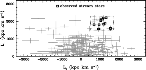
Figure 1.— Plot of the angular momentum components $L_{z}$ versus $L_{\perp}$. The data are mostly taken from Morrison et al. (2009) and supplemented with data from Chiba & Beers (2000) and Re Fiorentin et al. (2005) for some of the stream stars. The dotted box indicates the approximate range of angular momentum components of the stream members. The compiled data displayed here are intended to be representative of the distribution of angular momenta for stars in the disk and halo to illustrate the relative range of angular momenta occupied by the stream candidates. The unobserved stars in the box are RR Lyr stars or stars too faint to reasonably observe for our program.

To compute the orbit of an individual star, one needs to know its coordinates, distance, radial velocity, and proper motion; the position and space motion of the star can then be integrated over time in a model of the Galactic potential. Our study remeasures one of these quantities, the radial velocity, so we have checked our RV measurements against those employed by previous investigators to derive the kinematic properties of the stars. In some cases, the previous RV measurements were made from medium resolution spectra. If our high resolution RV measurements differ from the previous measurement, the original set of kinematic properties is suspect; fortunately, the difference can be quantified. It is also important that the stars are not in binary systems or, if they are, that the RV used to compute the kinematic properties is the systemic velocity. Comparing with previous high resolution and multi-epoch RV measurements by Latham et al. (1991), Carney et al. (2003, 2008), and Zhang et al. (2009), we confirm that this is the case. We retain all 12 candidates, listed in Table 2, as probable stream members. Below, we discuss a few candidates in more detail.

3.2. Comments on Individual Candidates

Beers et al. (1992) initially measured the RV of CS 22948–093 as 395 km s^-1, which was the value use to compute the original kinematics for this star. This star is RV variable over the 3-year baseline of our measurements, and the RV differs by approximately 30 km s^-1 from the Beers et al. (1992). From the definitions of $L_{z}$ and $L_{\perp}$ and the measured or derived stellar quantities from Beers et al. (2000), we can quantify the effect this RV difference has on the derived angular momenta, ($\Delta L_{z}$, $\Delta L_{\perp}$) $\approx$ (0, 200) kpc km s^-1. This is not sufficient to move CS 22948–093 from the main locus of probable stream members in Figure 1, so we retain it as a member.

Our abundance analysis of CS 29513–032 indicates that it has been polluted by material from a companion star that passed through the asymptotic giant branch (AGB) phase of evolution. (See Appendix A.) This implies that CS 29513–032 is in a binary or multiple star system, but we have detected no RV variations over a span of 3 months. Assuming that the star is in a binary system and that the systemic velocity is as much as 20 km s^-1 different from the measured RV would imply ($\Delta L_{z}$, $\Delta L_{\perp}$) $\approx$ (10, 160) kpc km s^-1. This is not sufficient to move CS 29513–032 much farther from the other probable members, so we also include this star as a member.

We made three observations of CS 29513–031 with a time interval of more than three years. Beers et al. (1992) measured a RV of 295 km s^-1 for this star. Our measurements indicate that this star is also RV variable, but the systemic velocity is not likely to be more than $\approx$ 10 km s^-1 different from the Beers et al. (1992) RV. If the systemic velocity is 10 km s^-1 different than the mean of the measured RV, ($\Delta L_{z}$, $\Delta L_{\perp}$) $\approx$ (300, 80) kpc km s^-1. CS 29513–031 is already located near the locus of probable members, and these uncertainties are small relative to the range of angular momenta for probable members, thus we also retain this star as a member.

4. Abundance Analysis

4.1. Linelist and Equivalent Width Measurement

We measure equivalent widths from our spectra using a semi-automatic routine that fits Voigt absorption line profiles to continuum-normalized spectra. Each measurement must be visually inspected and approved by the user. When possible, we use a single source for all of the log($gf$) values for a given species. References for our log($gf$) values are given in Table 3. Our equivalent width measurements and atomic data are presented in Table 4.

The Na i lines at 5889 and 5895 Å are often contaminated by telluric absorption features, and we have only measured equivalent widths for these lines when they appear to be velocity-shifted away from atmospheric components. We assess this by comparing the atmospheric transmission spectrum to the observed stellar spectrum. Additionally, the Na stellar lines may be blended with absorption or emission components from Na in the interstellar medium (ISM), and we only measure equivalent widths for these lines when no interstellar components are detected (e.g., as line asymmetries). We adopt the same technique to avoid telluric contamination to all lines redward of 5660Å, especially the high-excitation lines of Na i and Si i, which are often weak and might easily be mistaken for telluric absorption, and the K i resonance lines at 7664 and 7698Å.

4.2. Derivation of the Model Atmosphere Parameters

We perform the abundance analysis using the latest version (2009) of the spectral analysis code MOOG (Sneden, 1973). This version of MOOG incorporates the contribution of electron scattering in the near-UV continuum as true continuous opacity rather than extra absorption. (See Sobeck et al. 2010 for additional details.) Throughout our analysis we assume that all lines are formed under conditions of local thermodynamic equilibrium (LTE) in a one dimensional, plane parallel atmosphere.

Model atmospheres are interpolated from the grid of Castelli & Kurucz (2003), generated using the $\alpha$-enhanced opacity distribution functions assuming no convective overshooting. Atmospheric parameters are derived by spectroscopic means only. The effective temperature and microturbulence are determined by demanding that the derived Fe i abundances exhibit no trend with excitation potential or reduced equivalent width (i.e., equivalent width divided by wavelength). The resulting temperature and microturbulence generally satisfy these two criteria for the Fe ii and Ti i and ii abundances, though there are typically fewer lines of these species (8–11, 7–16, and 12–20 lines, respectively, compared with 80–120 lines for Fe i). These three species have a much more limited range of excitation potentials (typically $\sim$ 1 eV, compared with $\sim$ 4.5 eV for Fe i). The model surface gravity is determined by requiring that the Fe i and ii abundances agree within 0.1 dex (roughly the standard deviation of each). The model metallicities are set to the Fe abundance. The $\alpha$ elements are enhanced by a factor of 2–3 relative to Fe in our stars (Section 6). These elements are among the major electron donors to the H^- ion that dominates the continuous opacity over the visible spectral range, justifying our use of the $\alpha$-enhanced grid of atmospheres.

Figure 2 displays the evolutionary states of these stars, and Table 5 lists our derived model parameters. Six of them are found along the red giant branch (RGB), two are near the red horizontal branch (RHB), and four are on the subgiant branch (SGB) or main sequence turn-off. This range of evolutionary states will complicate inter-comparison of the absolute abundances; element-to-element ratios, however, should be more reliable, especially if the abundances are derived from lines of similar strength and thus are formed at similar levels of the atmosphere.

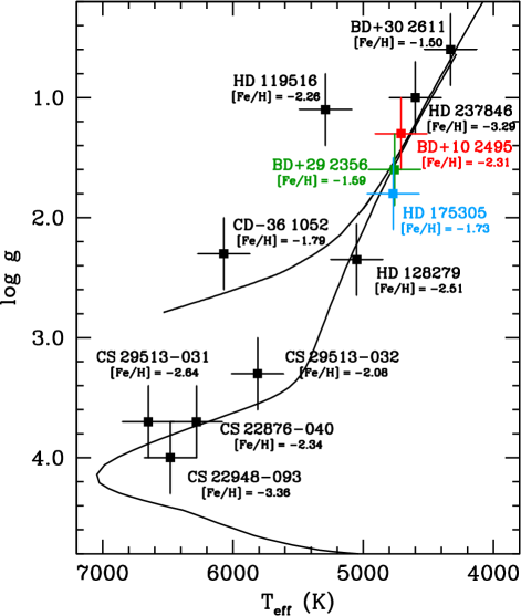
Figure 2.— Plot of the evolutionary states of the stream candidates. Our spectroscopically derived temperatures and gravities are shown, along with uncertainties of $\pm$ 200 K and $\pm$ 0.3 dex. Three stars along the RGB are color-coded to match the spectra displayed in Figure 3: BD$+$10 2356, BD$+$29 2495, and HD 175305. For comparison, a Y² $\alpha$-enhanced ([$\alpha$/Fe] $=+0.4$) 8 Gyr isochrone (Demarque et al., 2004) and a synthetic horizontal branch track for 0.8 M_⊙ (Cassisi et al., 2004) are shown, each computed for [Fe/H] $=-2.0$. Stream members are indicated as filled squares, and rejected candidates are indicated as “X”s.

In Table 6 we compare our spectroscopic temperatures to those derived from the infrared flux method (Alonso et al., 1999a, b) for five of the six stars on the RGB. The stars on the SGB and RHB are beyond the range of the calibrations. Five of the giants (BD$+$10 2495, BD$+$30 2611, HD 128279, HD 175305, and HD 237846) were included among the metal-poor calibration stars used by Alonso et al. (1999a), and we report their temperature estimates in Table 6. The spectroscopic and photometric $T_{\rm eff}$ estimates agree within the uncertainties for the coolest star in the sample, BD$+$30 2611, but for three of the other giants our spectroscopic estimates are cooler than the photometric ones by $\approx$ 250 K and the fourth is cooler by $\approx$ 380 K. This star, HD 237846, was also analyzed by Zhang et al. (2009), who derived a spectroscopic temperature of 4725 $\pm$ 60 K, which is only different from our estimate by 125 K.

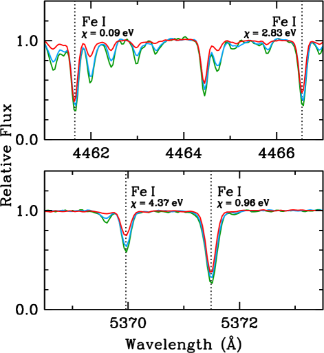
Figure 3.— Comparison of observed spectra for two pairs of Fe i lines with differing excitation potentials ($\chi$). Three stars along the RGB with very similar $T_{\rm eff}$ are shown: BD$+$10 2356, red ($T_{\rm eff}=$4710 K, [Fe/H]$=-$2.31); BD$+$29 2495, green (4760 K, [Fe/H]$=-$1.59); and HD 175305, blue (4770 K, $-$1.73). The colors also correspond to those used in Figure 2.

In Figure 3, we compare the spectra of three of the stars on the RGB with very similar temperatures but different metallicities. Two pairs of Fe i lines are shown, each with different excitation potentials. (By choosing line pairs at the same wavelength, we can compare line strength without the continuous opacity changing appreciably.) Our spectroscopic analysis shows that BD$+$10 2495, BD$+$29 2356, and HD 175305 all have temperatures within 60 K of one another, so to first order the largest difference in the line strengths in these stars is the Fe abundance; Figure 3 indicates that this is the case. Thus in a relative sense our temperatures are reasonable.

It is more difficult to assess the absolute temperature scale, but in a differential abundance analysis this effect is minimized as much as possible. In light of the discrepancies between the photometric and spectroscopic temperature scales, we adopt uncertainties on $T_{\rm eff}$, log $g$, and $v_{t}$ of 200 K, 0.3 dex, and 0.3 km s^-1. We adopt spectroscopic methods to estimate atmospheric parameters to avoid reliance on photometry (which may originate from a variety of sources, especially for bright stars) or models of the flux distribution (which must reproduce the energy distribution in stars of a variety of evolutionary states and compositions). Spectroscopically determined atmospheric parameters are certainly not without their own limitations, but the fact that most of the stars in Figure 2 lie along theoretical isochrones or HB tracks is reassuring in this regard.

4.3. Derivation of Abundances

For species with equivalent width measurements, we derive the abundance by forcing the individual line abundances to match the equivalent width and averaging over all lines. We match synthetic to observed spectra to derive abundances for species whose lines are broadened by hyperfine splitting, isotope shifts, or both, as well as for lines that are often weak or blended in our spectra (Li, Al, Sc, V, Mn, Co, Sr and all heavier elements). The C abundance is derived from a synthesis of the CH $A^{2}\Delta-X^{2}\Pi$ G-band between 4290 and 4330 Å, and the N abundance is derived from a synthesis of the CN $B^{2}\Sigma-X^{2}\Sigma$ bandhead region near 3880Å. For the odd-$Z$ Fe-peak species, we adopt the hyperfine structure patterns of Kurucz & Bell (1995). We use an $r$-process mix of Ba isotopes in our synthesis of the Ba ii 4554Å line for all stars except CS 29513–032, where we use an $s$-process mix (Appendix A). For all other Ba ii lines, the isotopic mix has no noticeable effect on the derived abundance. We adopt the hyperfine structure patterns for the rare earth elements from the references summarized in Lawler et al. (2009). Table 4 lists all of our equivalent width measurements or else indicates whether a line is used to determine an abundance via spectral synthesis or whether we compute an upper limit on the abundance from the line.

Abundances for all 12 stars are presented in Tables 7–10. Our main aim in this work is to compare the abundances of stars in the stream to each other and to other metal-poor populations. To this end, we do not apply any corrections to the abundances from our 1D LTE analysis to account for hydrodynamical motions or departures from LTE in the real atmospheres of these stars. We reference abundance ratios to the Solar abundances summarized in Asplund et al. (2009).

We assume a minimum uncertainty of 0.25 dex for abundances derived from a single spectral feature (set by statistical sources of error: our ability to resolve blending features, identify the continuum, measure an equivalent width or match a synthetic spectrum, etc.). For mean abundances derived from two lines, we adopt the larger of 0.15 dex or the standard deviation of a small sample as described by Keeping (1962). For mean abundances derived from more than two lines, we adopt the larger of of 0.10 dex or the standard deviation. We compute 3$\sigma$ abundance upper limits from the non-detection of absorption lines according to the formula given in Frebel et al. (2008), which was derived from Bohlin et al. (1983). These upper limits are indicated in Table 7–10.

5. Systematic Abundance Trends

It is important to recognize systematic differences that can bias results or mask real trends when performing detailed abundance comparisons. Stars of different metallicities or evolutionary states will naturally present different atomic transitions suitable for abundance analysis, and the abundances derived from these transitions need to be checked against one another. In this section we examine several systematic biases that could impact our results.

If the model atmosphere accurately reflects conditions in the stellar atmosphere, the abundance of elements not manufactured or destroyed during normal stellar evolution should show no dependence on $T_{\rm eff}$ when comparing stars with similar compositions but different temperatures. In Figures 4 and 5 we display the abundances of 30 species in our sample as a function of $T_{\rm eff}$. The depletion of the light element Li is evident in the more evolved (cooler) stars of the sample. The coolest star in the sample appears to have a slightly lower [C/Fe] ratio than the warmer stars. The CN band was only detected in one star. These trends are known consequences of normal stellar evolution. Correlations with $T_{\rm eff}$ are also detected for [Na i/Fe], [Ti i/Fe], and [V i/Fe]. These correlations will be discussed in the sections below.

Figure 4.— Abundances for Li i–V ii as a function of stellar effective temperature. Squares indicate measurements in the stream members and downward-facing triangles indicate upper limits. The dotted lines indicate the Solar ratio.

Figure 5.— Abundances for Cr i–Eu ii as a function of stellar effective temperature. Squares indicate measurements in the stream members and downward-facing triangles indicate upper limits. The dotted lines indicate the Solar ratio.

5.1. Silicon, Titanium, and Vanadium

In very metal-poor (or warm) stars, the only accessible line of Si i in the visible spectral range is the 3905Å line, which may become saturated in more metal-rich (or cooler) stars; this line has an excitation potential of 1.9 eV. In more metal-rich stars, high-excitation (4.9–5.1 eV) Si i lines at 5665, 5701, 5708, and 5772Å may be used as abundance indicators instead. In our sample, we only derive an abundance from the 3905Å line in the four warmest stars, while between 1 and 4 of the high-excitation lines are used in the cooler stars. The low- and high-excitation lines are not used together in any stars. As shown in Figure 4, the seven coolest stars ($T_{\rm eff}<$ 6000 K) with detected Si i lines all employ the high-excitation lines and show a slope of decreasing [Si i/Fe] with decreasing temperature. This trend is in the opposite sense from what previous studies have uncovered. In contrast, the four warmest stars ($T_{\rm eff}>$ 6000 K) all employ the 3905Å line and may show a slope of increasing [Si i/Fe] with decreasing temperature, which has been recognized by previous investigators (Cohen et al., 2004; Preston et al., 2006; Lai et al., 2008; Bonifacio et al., 2009). Using only abundances derived from the 3905Å line, Preston et al. (2006) compared the [Si/Fe] ratio in stars on the lower RGB to stars on the RHB (i.e., with the same temperature but different gravities) and found no dependence on gravity, implying that this observed difference is not a consequence of stellar evolution. In addition to noting this trend of increasing [Si i/Fe] with decreasing temperature, Lai et al. (2008) also identified opposite trends for [Ti i/Fe] and [Ti ii/Fe].

We also find a weak trend of increasing [Ti i/Fe] and increasing [V i/Fe] with increasing $T_{\rm eff}$ in our sample. The Ti i abundance is derived from $\sim$ 5–15 lines, suggesting that this trend is not a consequence of line blending. The V i abundance is derived from a single transition, 4379.23Å. The direction of this trend, increasing [V i/Fe] with increasing $T_{\rm eff}$, would imply that the blending feature is decreasing in line strength with increasing $T_{\rm eff}$. No plausible blending atomic features are found in the Kurucz linelists or the NIST database. A ¹²CH transition at 4379.24Å could, in principle, produce the observed effect, although our syntheses indicate that completely removing the contribution from CH even in the giants will increase the V i abundance by no more than 0.01–0.02 dex, far smaller than the observed abundance change with $T_{\rm eff}$. We have not investigated the consequences of including 3D effects or departures from LTE in the line formation.

In summary, it it not clear what causes these trends, but they do not appear to be the result of any shortcomings unique to our analysis. Further investigation of the [Si i/Fe] (high-excitation lines), [Ti i/Fe], and [V i/Fe] abundance trends with $T_{\rm eff}$ is beyond the scope of this work. Whatever the cause, it is responsible for producing the larger star-to-star dispersion in these ratios than observed for other species that show no correlation with $T_{\rm eff}$.

5.2. Magnesium

The Mg i transitions at 3829, 5172, and 5183Å have $\chi\approx$ 2.7 eV, and the Mg i lines at 4057, 4167, 4702, 5528, and 5711Å have $\chi\approx$ 4.3 eV. This fact manifests itself as a difference in line strengths. In warm or very metal-poor stars, only the lower-excitation lines are strong enough to be detected. For Mg, we derive abundances from the 5172 and 5183Å lines in four stars, three of which also use several of the high-excitation lines (CS 22876–040, CS 29513–031, and HD 237846, two stars on the SGB and one on the RGB). In these three cases, the 5172 and 5183Å lines yield abundances higher than the high-excitation lines by 0.13, 0.29, and 0.23 dex, respectively. Cohen et al. (2004) examined this effect in seven metal-poor dwarf stars from their sample. After correcting for the differences in log($gf$) values between the two studies, their mean offset, 0.26 dex, is very similar to ours. The 5172 and 5183Å lines also yield abundances higher than the 3829Å line by 0.32, 0.26, and 0.14 dex in CS 22876–040, CS 22948–093, and HD 237846 (again, two stars on the SGB and one on the RGB). We find no dependence of [Mg/Fe] on $T_{\rm eff}$ in Figure 4.

We have derived Mg i abundances from at least 2 high-excitation lines in all but one star, so we only adopt the Mg abundance derived from these lines. Only in CS 22948–093, where no high-excitation lines were measured, do we employ the low-excitation lines. We omit this star when computing the [Mg/Fe] dispersion in the stream.

5.3. Manganese

The Mn i resonance triplet at 4030, 4033, and 4034Å has an excitation potential of 0.0 eV, and the Mn i lines farther to the red have excitation potentials ranging from 2.1–3.1 eV. The triplet lines are the only Mn i abundance indicators in the optical regime for very metal-poor stars. The Mn i triplet is known to yield abundances lower by 0.3–0.4 dex relative to the higher-excitation Mn i lines (e.g., Cayrel et al. 2004). This effect is also observed in our sample, with an average difference of $-$0.32 dex when both the triplet and the higher-excitation lines are detected and measurable (6 stars). To compare relative [Mn i/Fe] abundances for stars in our sample, we correct all of the Mn i triplet abundances by $+$0.3 dex. This correction is reflected in Tables 7–10. We emphasize that this is strictly an empirical correction. In one star from our sample, HD 128279, we were also able to derive an abundance of Mn ii from the 3488 and 3497Å lines. We are encouraged that the abundance derived from these lines, log $\epsilon$ (Mn ii) $=+2.56$ dex, is in very good agreement with the Mn i abundance derived from the high-excitation lines, log $\epsilon$ (Mn i) $=+2.52$ dex.

5.4. Sodium

The Na i resonance lines at 5889 and 5895Å have $\chi=$ 0.0 eV, while the 5682 and 5688Å lines have $\chi\approx$ 2.1 eV. Only the 5889 and 5895Å lines are detected in warm or very metal-poor stars. We only derive an abundance from the 5889Å line in one star, CS 29513–031, and we derive an abundance from the 5895Å line in only one star, CS 29513–032. All other Na abundances are derived from the 5682 and 5688Å lines, which are in very good agreement with one another. We omit CS 29513–031 and CS 29513–032 when computing the [Na/Fe] dispersion in the stream.

5.5. Other Elements

Abundances are derived from the resonance line pairs of Al i (3944 and 3961Å), K i (7664 and 7698Å), and Sr ii (4077 and 4215Å), as well as the high-excitation lines of Zn i (4722 and 4810Å). For each of these species, these lines are the only abundance indicators available to us. In cases where both lines are measured, we find no systematic offsets from one line to the next for Al, K, and Zn.

Both Sr ii resonance lines were measured in 10 stars, and we find that the 4077Å line gives an abundance lower by 0.08 ($\sigma=$ 0.04) dex than the 4215Å line. The offset is smaller in the stars on the SGB (0.05 dex) than stars on the RGB or RHB (0.09 dex), suggesting that this offset may originate, at least in part, in modeling the line formation, as opposed to a systematic offset in the log($gf$) values. These Sr lines are often very strong and are blended at this metallicity range, with observational uncertainties often 0.2–0.3 dex, so this finding should be viewed with necessary caution. We make no correction to the Sr ii abundances here, but this possible systematic effect should be investigated further in larger samples at low metallicity where the blending is less severe and the Sr lines less saturated.

6. Abundances in the Stream Stars

Our derived [X/Fe] abundance ratios for the probable stream members are shown in Figures 6–10. The stream members range in metallicity from $-3.4\leq$ [Fe/H] $\leq-1.5$, and they are not unique with respect to the rest of the halo in this regard. In these figures, CS 29513–032 is indicated separately because its abundances for $Z\leq$ 11 and $Z\geq$ 29 may not reflect their primordial (birth) abundances. These abundances in CS 29513–032 are excluded from the star-to-star chemical dispersions discussed in the following sections, but the species with 12 $\leq Z\leq$ 28 have been included.

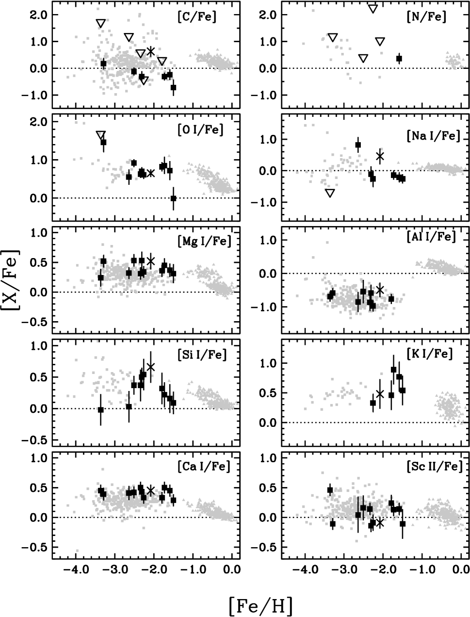
Figure 6.— Abundance ratios [X/Fe] for C–Sc ii as a function of metallicity. Large filled squares indicate measurements in the stream members and downward-facing triangles indicate upper limits. CS 29513–032 is indicated by the “X.” Gray triangles indicate thin and thick disc stars (Reddy et al., 2003, 2006). Gray squares indicate field halo stars (Cayrel et al., 2004; Barklem et al., 2005; Cohen et al., 2008; Lai et al., 2008). The Solar ratio is indicated in each panel by the dotted line.

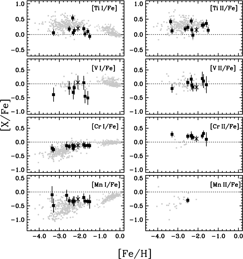
Figure 7.— Abundance ratios [X/Fe] for Ti i–Mn ii as a function of metallicity. Symbols are the same as in Figure 6.

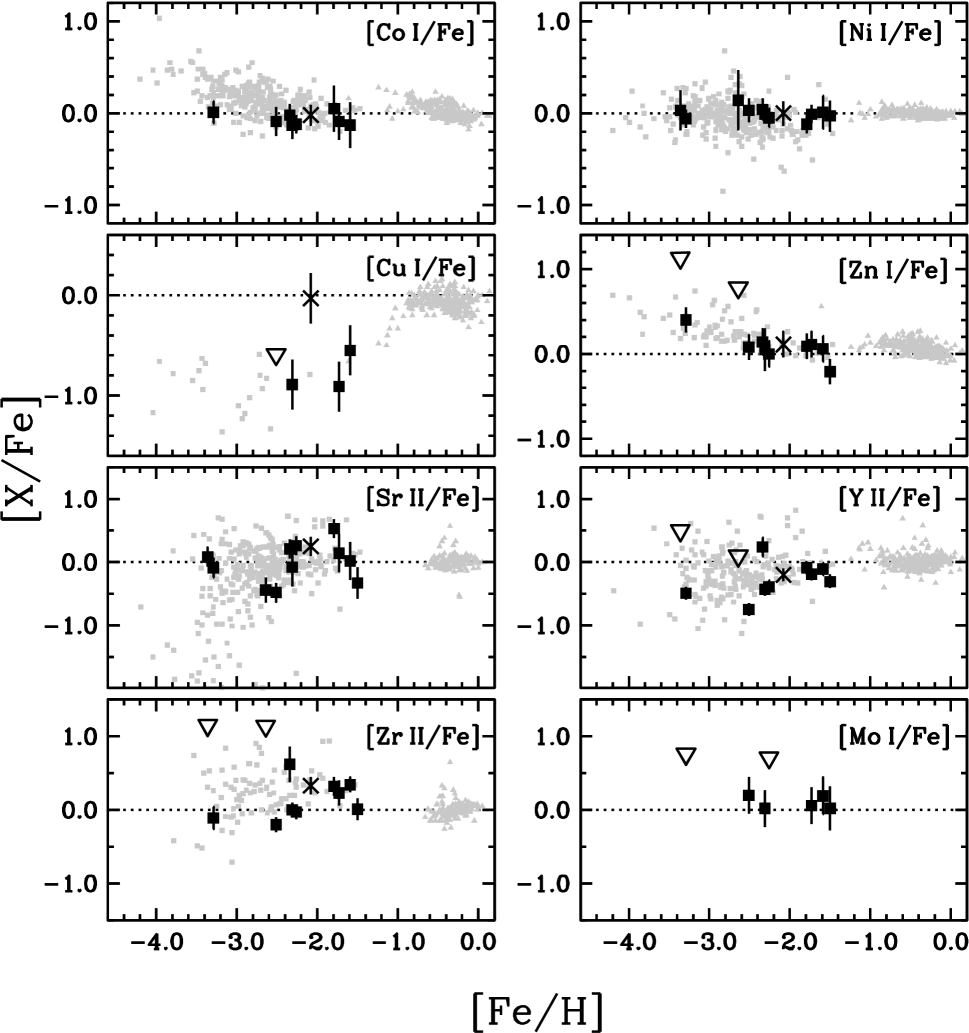
Figure 8.— Abundance ratios [X/Fe] for Co i–Mo i as a function of metallicity. Symbols are the same as in Figure 6 and include abundances from François et al. (2007).

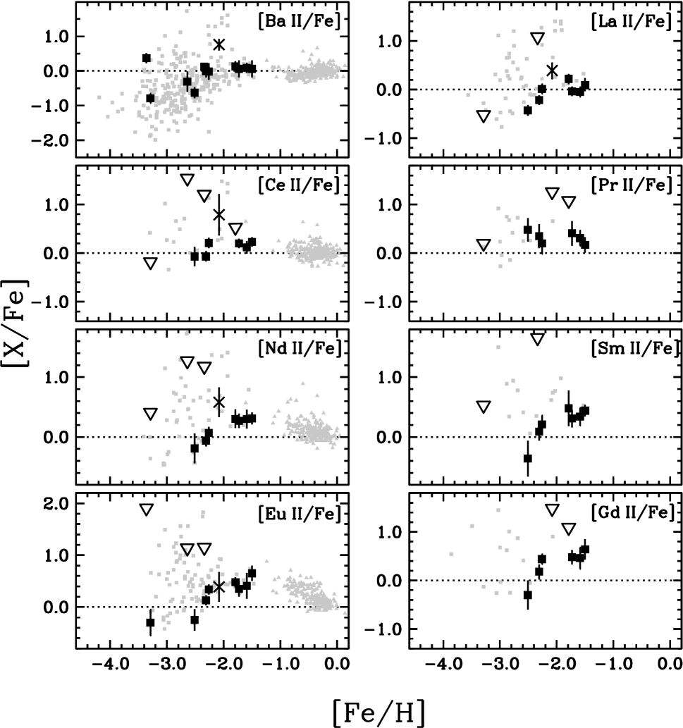
Figure 9.— Abundance ratios [X/Fe] for Ba ii–Gd ii as a function of metallicity. Symbols are the same as in Figure 6.

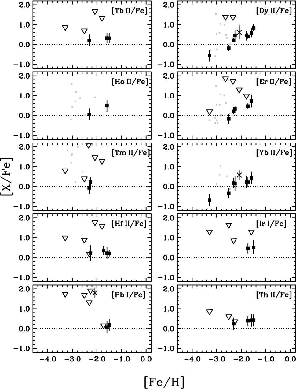
Figure 10.— Abundance ratios [X/Fe] for Tb ii–Th ii as a function of metallicity. Symbols are the same as in Figure 6.

6.1. Carbon to Zinc

The [C/Fe] ratios for the stream members are all sub-Solar by a factor of 2–3. [O/Fe] is super-Solar and similar to other metal-poor stars in the halo. The [Na i/Fe] and [Al i/Fe] ratios are both sub-Solar, suggesting that Na and Al have not been enriched by the CNO, NeNa, and MgAl cycles like stars found in globular clusters. The Al non LTE (NLTE) line formation corrections suggested by Andrievsky et al. (2008) for the 3961Å line would increase the [Al i/Fe] ratios to Solar or just slightly sub-Solar, but the overall relative abundances are basically unchanged. The star-to-star dispersions (standard deviation) are 0.29 dex for [C/Fe], 0.07 dex for [Na i/Fe], and 0.17 dex for [Al i/Fe].

The $\alpha$ elements (O, Mg, Si, Ca, and Ti) are all enhanced relative to Fe at levels similar to other stars in the halo. The dispersion for [O i/Fe] is 0.36 dex, although this drops to 0.13 dex if only two stars (BD$+$30 2611 and HD 237846) are excluded. The dispersions are similarly small for [Mg i/Fe] (0.10 dex) and [Ca i/Fe] (0.07 dex); the somewhat larger dispersion for [Si i/Fe] (0.16 dex) and [Ti i/Fe] (0.17 dex) can be attributed to the $T_{\rm eff}$ correlations found in Section 5.1. [Ti ii/Fe] shows no such $T_{\rm eff}$ correlation, so the larger scatter observed here (0.14 dex) may be genuine. If we ignore [Si i/Fe], the stream members show no evolution in their [$\alpha$/Fe] ratios over nearly 2 dex in [Fe/H].

The [K i/Fe] ratios are super-Solar and show no evolution over $-2.3\leq$ [Fe/H] $\leq-1.5$ within the observational uncertainties. Ivanova & Shimanskiĭ (2000) and Takeda et al. (2009) computed NLTE corrections for the optical K i resonance lines for metal-poor stars, and both groups found corrections of $-$0.20 to $-$0.35 over the evolutionary states of our sample. Thus our overall [K i/Fe] ratio may need to be revised downward by a factor of $\sim$ 2 (as should the other metal-poor stars illustrated in Figure 6), but this should have minimal impact on the star-to-star dispersion (0.21 dex).

The [Sc ii/Fe] and [V ii/Fe] ratios for the stream members are roughly Solar. Both exhibit moderate dispersions (0.18 and 0.13 dex, respectively). The large [V i/Fe] dispersion (0.21 dex) is a consequence of the $T_{\rm eff}$ dependence.

The [Cr i/Fe] and [Cr ii/Fe] ratios show very small star-to-star dispersion (0.05 and 0.07 dex, respectively), and the and [Cr i/Fe] ratios are $\approx$ 0.3–0.4 dex lower than the [Cr ii/Fe] ratios. Sobeck et al. (2007) reexamined the transition probabilities and Solar abundance of Cr i, finding that the [Cr i/Fe] ratios were 0.15–0.20 dex lower than the [Cr ii/Fe] ratios. Yet Sobeck et al. (2007) found no compelling evidence that this discrepancy was due to NLTE effects, and their stellar sample suggested that the Cr i and Cr ii abundances may be more discrepant at lower metallicities; our results qualitatively support this conclusion, although this does not imply which set of stellar [Cr/Fe] ratios (if either) should accurately reflect the true value.

The [Mn i/Fe] ratios for the stream members are sub-Solar by a factor of 2, show no evolution over the metallicity range, and have a very small dispersion (0.11 dex). This last attribute is not a consequence of our decision to adjust the abundance of the resonance lines by $+$0.3 dex: the dispersion in [Mn i/Fe] derived from only the higher-excitation lines is only 0.06 dex (8 stars). Thus the small dispersion in [Mn i/Fe] is intrinsic.

[Co i/Fe], [Ni i/Fe], and [Zn i/Fe] are all Solar (within 0.1 dex), have small or moderate dispersions (0.07, 0.06, and 0.16 dex, respectively), and show no evolution with metallicity (with the possible exception of Zn in HD 237846). The [Cu i/Fe] ratio was only derived for three stars (plus CS 29513–032). For these three stars, the [Cu i/Fe] ratio is in good agreement with other stars in the halo, and the dispersion is moderate, 0.20 dex.

How does the star-to-star dispersion observed in the stream members compare with the rest of the halo? In Figure 11 we illustrate the dispersion in the various [X/Fe] ratios and compare with the dispersion computed for metal-poor red giants in the sample of Cayrel et al. (2004). Table 11 lists these values. The Cayrel et al. (2004) sample was optimized to measure the true cosmic dispersion (i.e., with observational uncertainties minimized) of the very metal-poor end of the Galactic halo. The stream spans a metallicity range of $-3.4<$ [Fe/H] $<-1.5$, so we only compare with the metal-rich end of this sample ($-3.4<$ [Fe/H] $<-2.0$) We do not attempt to compare abundance ratios that exhibit a dependence on $T_{\rm eff}$ in our sample. On average, the dispersion in the stream is comparable to or smaller than the dispersion of the two datasets of halo giants. The implications of this point will be discussed further in Section 7.1.

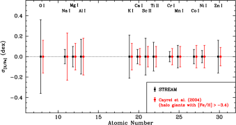
Figure 11.— The star-to-star dispersion in [X/Fe] ratios for the stream members compared with the Cayrel et al. (2004) sample of metal-poor halo giants. Only the halo giants with [Fe/H] $>-3.4$ have been included. Abundance ratios that show a dependence on $T_{\rm eff}$ in the stream members ([Si i/Fe] and [Ti i/Fe]) have been excluded.

6.2. Strontium to Thorium

In this section, we will ignore CS 29513–032, whose heavy element abundances likely do not represent their initial values. For the remaining stream stars, most of the heavier elements follow similar patterns to the $\alpha$- and Fe-group elements, with one clear distinction: the stream members with [Fe/H] $>-2.2$ show a constant value of [X/Fe] (X stands for Ba and all heavier elements in this case). These values range from $\approx$ Solar (Ba, La) to $\approx$ 3–4 times Solar (e.g., Eu, Gd, Dy, Er). The stream members with [Fe/H] $<-2.2$ show gradually increasing [X/Fe] ratios with increasing [Fe/H] that appear to culminate near the [X/Fe] ratios of the more metal-rich stars. The lighter elements Y and Zr show similar trends, but one star (CS 22876–040, [Fe/H] $=-2.34$) stands out with [Y ii/Fe] and [Zr ii/Fe] ratios $\approx$ 0.6 dex higher than the other stars with [Fe/H] $=-2.3$. Otherwise the [Y ii/Fe] and [Zr ii/Fe] ratios for the stars with [Fe/H] $<-2.2$ show a gradual increase of [X/Fe] with increasing [Fe/H]. [Y ii/Fe] and [Zr ii/Fe] show dispersions of 0.10 and 0.15 dex among the stars with [Fe/H] $>-2.2$. The [Sr ii/Fe] ratio shows a moderate dispersion (0.31 dex) at all metallicities. The [Mo i/Fe] ratio shows no evolution with metallicity and has a dispersion of 0.09 dex.

Production of the elements heavier than the Fe-group occurs primarily by successive neutron ($n$) captures on existing nuclei. The resulting abundance patterns are largely determined by the rate of neutron captures, either slow ($s$) or rapid ($r$) relative to the nuclear $\beta^{-}$ decay rates. The general abundance patterns of these two processes are relatively well known, and they can be readily identified when one process dominates the production of the heavy isotopes. Relatively large amounts of material tend to build up when either $n$-capture process encounters closed nuclear shells at $N$ (or $Z$) $=$ 50, 82, or 126; these relative overabundances are commonly referred to as the 1^st, 2^nd, and 3^rd peaks, respectively.

One of the surprising results of many detailed investigations of $n$-capture abundances in metal-poor stars over the last 15 years has been the near-perfect match between the stellar distribution for the rare earth elements (La–Yb), 3^rd peak elements (Os–Pt), and actinides (Th) and the scaled-Solar $r$-process distribution. This agreement has only improved with better atomic data (Sneden et al., 2009). This pattern is observed in many stars in different populations that must be enriched by separate events. The constant $n$-capture-element to $n$-capture-element ratios do not extend to material at the 1^st $r$-process peak (e.g., Truran et al. 2002).

In Figure 12 we show the abundance distribution for the $n$-capture material in one stream star, BD$+$10 2495. Three $n$-capture enrichment templates are shown for comparison: the main component of the $r$-process (exemplified by the well-studied star CS 22892–052), the main component of the $s$-process (exemplified by the Solar-metallicity model of the $s$-process from Arlandini et al. 1999), and the so-called weak component of the $r$-process (exemplified by the well-studied star HD 122563). The curves are normalized to one another at the Eu abundance. For the heaviest elements ($Z\geq$ 62), the abundance pattern very clearly follows the main component of the $r$-process—even though the [Eu/Fe] ratio is only $+$0.1 relative to the Solar ratio. For the light rare earth elements (56 $\leq Z\leq$ 60), the abundances lie near but slightly above the main component of the $r$-process and close to the weak component of the $r$-process. The light $n$-capture elements (38 $\leq Z\leq$ 42) also fall between the weak and main components of the $r$-process, though usually tending towards the weak component. A pure $s$-process is clearly ruled out.

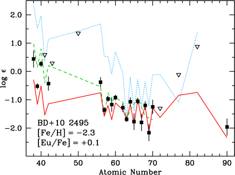
Figure 12.— Neutron-capture abundances for BD$+$10 2495. Squares indicate measurements and open triangles indicate upper limits. Abundances for CS 22892–052 (the template for the main component of the $r$-process, shown as a solid line) have been adopted from Sneden et al. (2003a, 2009), abundances for HD 122563 (the template for the weak component of the $r$-process, dashed line) have been adopted from Honda et al. (2007), and the $s$-process abundances (dotted line) are taken from the Solar metallicity stellar model of Arlandini et al. (1999). The curves are normalized to the Eu abundance.

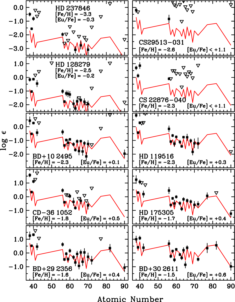
Figure 13.— Neutron-capture abundances for ten of the stream members. (Regarding the other two members: CS 29513–032 is analyzed in detail in the Appendix, and only the Sr ii and Ba ii abundances were derived for CS 22948–093.) Squares indicate measurements and open triangles indicate upper limits. Abundances for CS 22892–052 (the template for the main component of the $r$-process, shown as a solid line) have been adopted from Sneden et al. (2003a, 2009). The curve is normalized to the Eu abundance in each star, with the exception of CS 29513–031 and CS 22876–040 (Eu upper limit), where the curve scaling is approximately matched to the Ba abundance offset observed in the remaining stars.

Similar plots are shown for ten stream members in Figure 13, except here only the template for the main component of the $r$-process is shown to reduce clutter. Clearly, in all cases where at least a few $n$-capture elements can be detected, the enrichment pattern is virtually identical to that in BD$+$10 2495.

Stars enriched in $s$-process material by companions that passed through the AGB phase of evolution are also enriched in C (Sneden et al., 2003b), which is not the case for any of the stream members. Furthermore, no stream members have high [Pb/Fe] ratios. An enhanced Pb ($Z=$ 82) abundance will be the first detectable signature of the $s$-process at low metallicity. At low metallicity, due to the higher ratio of neutrons to Fe-group seed nuclei for the $s$-process, models predict that a low metallicity $s$-process produces large Pb/Fe and Pb/2^nd peak ratios relative to higher metallicity $s$-process models (e.g., Gallino et al. 1998). This has been confirmed by a number of observational studies (e.g., Van Eck et al. 2003, Ivans et al. 2005). If the observed $n$-capture abundance pattern in the stream stars were to result from the combination of material produced in the main component of the $r$-process and the main component of the $s$-process, we would expect to detect large Pb/2^nd peak ratios in these stars. In the two stars where Pb is detected (BD$+$29 2356 and BD$+$30 2611)—the two most metal-rich stars in our stream sample—the Pb abundance clearly matches the pure $r$-process pattern. The Pb upper limit in HD 175305 also strongly suggests an $r$-process origin.

We conclude that the $n$-capture material was produced by the main component of the $r$-process with significant contributions from the weak component of the $r$-process at the 1^st peak and light end of the rare earth domain. There is no evidence that any of the material in the stream stars originated in the $s$-process.

7. Discussion

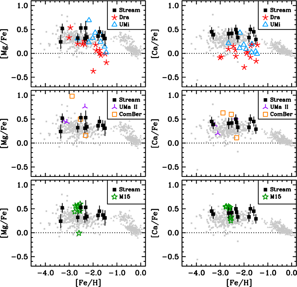
Figure 14.— Abundance ratios [Mg/Fe] and [Ca/Fe] for the stream stars and select other stellar populations. Gray triangles indicate thin and thick disc stars (Reddy et al., 2003, 2006). Gray squares indicate field halo stars (Cayrel et al., 2004; Barklem et al., 2005; Cohen et al., 2008; Lai et al., 2008). Abundances for the Ursa Minor dSph are taken from Shetrone et al. (2001), Sadakane et al. (2004), and Aoki et al. (2007). Abundances for the Draco dSph are taken from Shetrone et al. (2001), Fulbright et al. (2004), and Cohen & Huang (2009). Abundances for the Coma Berenices and Ursa Major II uFds are taken from Frebel et al. (2010). Abundances for globular cluster M15 are taken from Sobeck et al. (2010). The Solar ratio is indicated in each panel by the dotted line.

7.1. The Chemical Nature of the Stream

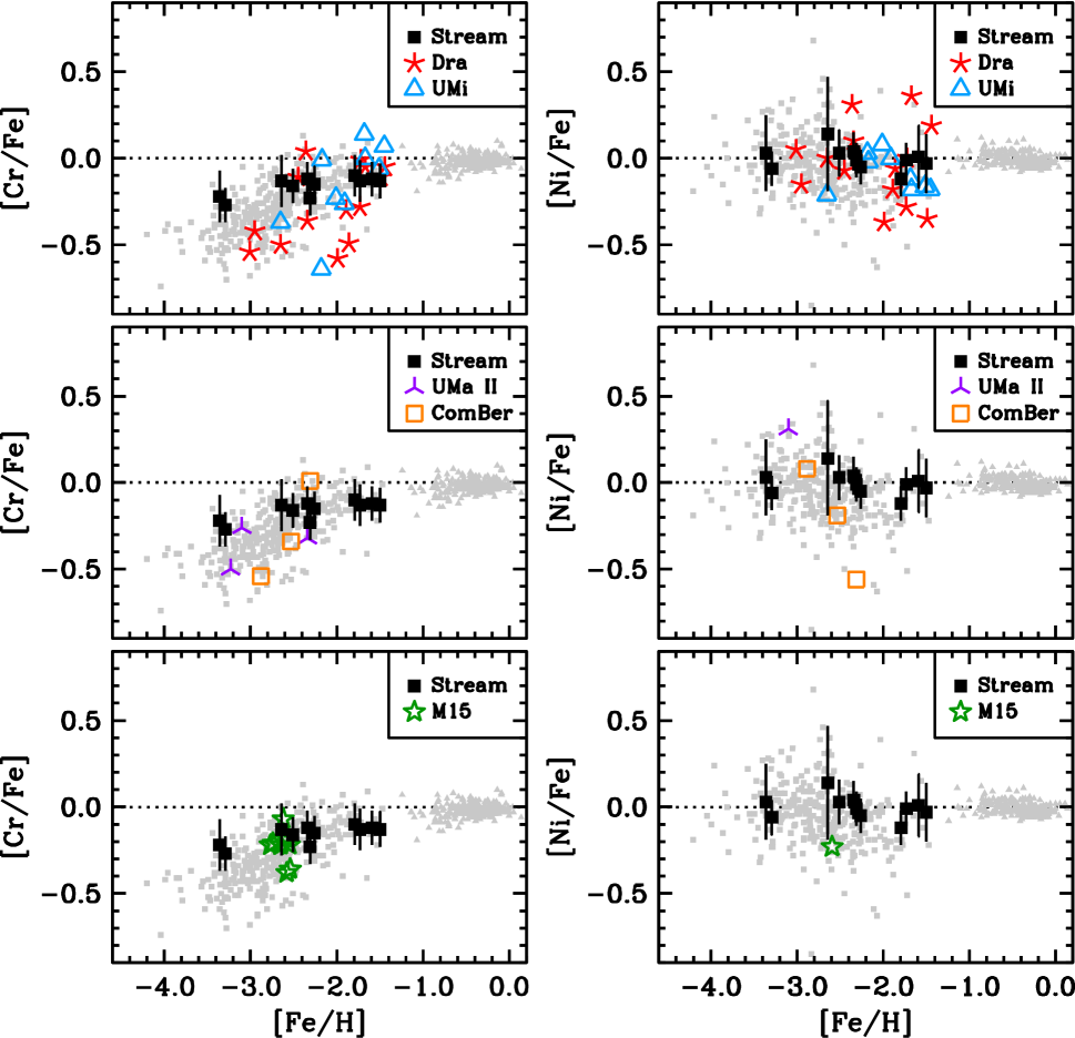
Figure 15.— Abundance ratios [Cr/Fe] and [Ni/Fe] for the stream stars and select other stellar populations. Symbols are the same as in Figure 14.

The abundance pattern in the stream stars appears to be the result of massive Type II supernovae, characterized by sub-Solar [C/Fe] and enhanced [$\alpha$/Fe] ratios. The [Fe/H] abundances span almost 2 dex, but the [X/Fe] ratios for the $\alpha$ and Fe-group elements are basically unchanged. The $n$-capture elements are the lone exception, showing Solar or sub-Solar ratios at the lowest metallicities in the stream but increasing to a super-Solar plateau at the highest metallicities. One proposed site for the $r$-process is the high-entropy wind of $\sim$ 8–10 $M_{\odot}$ Type II supernovae, which may be capable of producing both the weak and main components of the $r$-process (e.g., Farouqi et al. 2009). This scenario seems to imply that the lowest metallicity stream stars ([Fe/H] $\lesssim-2.2$) were formed from gas polluted by more massive Type II supernovae, while the more metal-rich stars ([Fe/H] $\gtrsim-2.2$) were formed from gas polluted by less-massive Type II supernovae. Subsequent generations of supernovae then continue to enrich the ISM, but star formation appears to have been truncated before the yields of Type Ia supernovae or AGB stars contributed significantly to the chemical inventory. This would also imply that whatever site is responsible for producing the $r$-process does not produce a difference in the light element ($Z\leq$ 30) production ratios from the sites that do not produce an $r$-process.

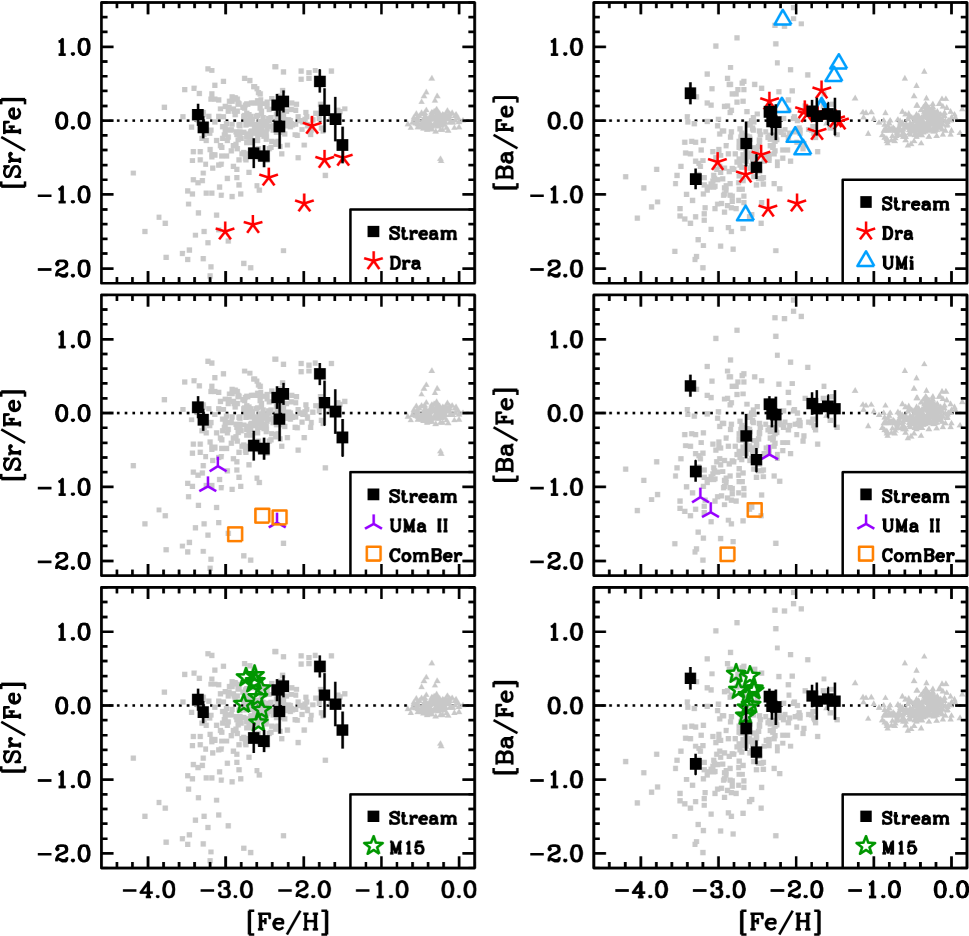
Figure 16.— Abundance ratios [Sr/Fe] and [Ba/Fe] for the stream stars and select other stellar populations. Symbols are the same as in Figure 14.

In Figures 14, 15, and 16 several abundance ratios for the stream stars are compared with analogous abundance ratios of other stellar populations. These include field stars in the thin and thick disc populations, halo stars, two dSph galaxies (Draco and Ursa Minor), two uFds (Coma Berenices and Ursa Major II), and the metal-poor globular cluster M15. At a given metallicity, the stream shows an equal or smaller star-to-star dispersion in [X/Fe] when compared with stars in the dwarf galaxies. Furthermore, the dwarf galaxies show evolution in their [X/Fe] ratios as a function of metallicity (e.g., Mg or Cr); the stream only shows such evolution for the $n$-capture elements. The $n$-capture elements show significantly larger dispersion in these dwarf galaxies than in the stream, with the dwarf galaxy dispersions often reaching 1–2 dex at a single metallicity.

The Sgr dSph (not illustrated in these Figures) is much more metal-rich than the stream and shows clear evidence for a large dispersion and evolution of several [X/Fe] ratios with metallicity (e.g., Monaco et al. 2005, 2007; Sbordone et al. 2007). Majewski et al. (2003) argue that this particular stream cannot be related to Sgr debris because its $R_{\rm apo}$ is too small and its $L_{z}$ angular momentum is too high. Furthermore, Sgr contributes less than 1% of the evolved halo stars in the Solar neighborhood, and the Sgr debris would not have significantly impacted the kinematic studies that have detected the presence of this stream. We reaffirm this conclusion on the basis of the composition of the stream stars.

The stream does not resemble a globular cluster in that it shows a range of metallicities spanning nearly 2 dex, whereas globular clusters, such as M15, show minimal or no internal metallicity spread (except for $\omega$ Centauri). The stream also does not resemble a dSph or uFd system, whose [X/Fe] ratios show much larger star-to-star dispersion and evolution of the [X/Fe] ratios as a function of [Fe/H] (insofar as the true chemical dispersion can be estimated for the uFd systems from measurements of only 3 stars in each of two systems; Frebel et al. 2010). The luminous dSph systems spend—at most—a very small fraction of their lives in the Solar neighborhood (Roederer, 2009), so these particular systems would not be expected to have spawned the stream. The stream has the same chemical dispersion as the rest of the local halo, and it is reasonable to hypothesize that, in principle, a significant fraction of field halo stars (at least those currently in the Solar neighborhood) could form in progenitor systems like that from which the stream originated.

Two stars in the stream have [Fe/H] $<-3.0$, HD 237846 ([Fe/H] $=-3.3$) and CS 22948–093 ([Fe/H] $=-3.4$). While it is possible that these stars have no association with the stream yet by pure chance have similar kinematics, there is no a priori reason to exclude them from membership on these grounds. Multiple enrichment events spanning multiple stellar generations are required to enrich an unpolluted ISM to a metallicity of [Fe/H] $=-1.5$, the metal-rich end of our stream stars. Therefore, it is reasonable to expect that at least a few stars with [Fe/H] $<-3.0$ formed in the stream’s progenitor system throughout the enrichment process. Furthermore, the [X/Fe] abundance ratios in these two stars are generally consistent with the other stream members. In the last few years a number of stars with [Fe/H] $<-3.0$ have been identified in dwarf galaxies (Cohen & Huang, 2009; Frebel et al., 2010; Geha et al., 2009; Kirby et al., 2009; Norris et al., 2009). If a significant fraction of the stellar halo is postulated to be formed by the accretion of satellites like the stream’s (unidentified) progenitor, we should not be surprised to encounter stream stars with [Fe/H] $<-3.0$.

7.2. Stellar Ages from Nuclear Cosmochronometry

We have detected Th in four stream members, which permits us to estimate the ages of these stars by comparing the abundance of Th (which is radioactive with a halflife $t_{\rm 1/2}[^{232}{\rm Th}]=14.05\,\pm\,$0.06 Gyr; Audi et al. 2003) to another stable element produced in the same nucleosynthesis event. Th can only be produced by the main $r$-process, and in this stream the Eu has also only produced by the main $r$-process. By referencing the current Th/Eu ratio against the expected production ratio (e.g., Kratz et al. 2007) an age for the $r$-process material (and an upper limit for the age of the stars themselves) can be calculated. The mean age for the four stars in the stream is 3.1 $\pm$ 7.9 Gyr, and this uncertainty is dominated by the star-to-star dispersion in Th/Eu.

This large uncertainty prevents us from making any meaningful statements about the age of the stream, and the mean age is uncomfortably small for metal-poor stars. The Th ii abundance has been derived from a single transition in each of the stream stars, and this line is always weak ($\sim$ 5 mÅ) and blended with other features. The Th/Eu ratios for three of the stars (BD$+$10 2495, BD$+$29 2356, HD 175305) are higher than the fourth (BD$+$30 2611); the Th abundance in the former three stars was derived from the 4019Å line, while the 4094Å line was used in the latter due to severe blending at the 4019Å line. Roederer et al. (2009) found no systematic difference in the Th abundance derived from these lines. Our syntheses of the 4019Å Th ii line are shown in Figure 17.

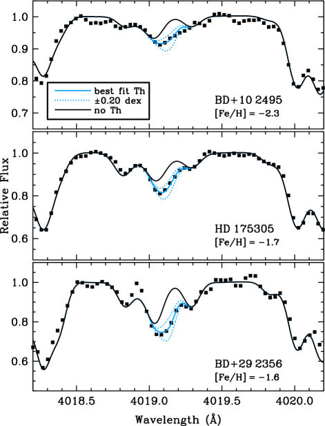
Figure 17.— Syntheses of the Th ii line in the three stars where we have used this line to derive the Th abundance.

There are currently four metal-poor field stars with exceptionally high Th/Eu ratios. In the one star in this class with detected U, CS 31082–001, the U/Th ratio gives a reliable age, while the U/$r$ and Th/$r$ ratios (where $r$ is any reference element) predict negative ages (Hill et al., 2002; Plez et al., 2004). This so-called “actinide boost” (Schatz et al., 2002), which seems only to affect the $r$-process material heavier than the 3^rd $r$-process peak (Roederer et al., 2009), is characterized by low Pb and enhanced Th and U (relative to the majority of $r$-process enriched metal-poor stars). This nucleosynthetic idiosyncrasy is unexplained by current models of the $r$-process. We do not detect U in any of these stars, nor can we place a meaningful upper limit on its abundance. The Pb abundance in two of these stars is normal (i.e., consistent with no actinide boost), and the Pb upper limit in the other two cannot exclude a normal Pb abundance. The actinide boost phenomenon does not seem to be able to explain the high Th/Eu ratios in these stars.

It is possible that these stars (and the $r$-process material in them) may be younger than the rest of the halo, but we urge caution in interpreting the ages calculated from abundances derived from a single, weak, and blended Th feature in each of these stars. Postulating that some fraction of the Eu was formed via the weak $r$-process (instead of the main component of the $r$-process, which produces the Th) only exacerbates the age discrepancy.

8. Conclusions

We have performed a detailed abundance analysis of 12 metal-poor halo field stars whose kinematics suggest they are members of the stellar stream first discovered by Helmi et al. (1999). These stars exhibit a range of metallicity ($-3.4\leq$ [Fe/H] $\leq-1.5$) but are otherwise chemically homogeneous for elements with $Z\leq 30$. The [$\alpha$/Fe] ratios are enhanced to levels typical for stars in the local Galactic halo (e.g., [Mg/Fe] or [Ca/Fe] $=+0.4$). The star-to-star dispersion in [X/Fe] is very small and the same as found for other halo field stars (e.g., the sample of metal-poor giants analyzed by Cayrel et al. 2004). The $n$-capture elements are deficient at the lowest metallicities (e.g., [Ba/Fe] $=-0.8$ or [Eu/Fe] $=-0.3$) but increase and plateau at the highest metallicities (e.g., [Ba/Fe] $=0.0$ or [Eu/Fe] $=+0.4$). The $n$-capture elements are clearly produced by the main and weak components of the $r$-process, and there is no evidence for enrichment by the $s$-process. These enrichment patterns can be produced by Type II core-collapse supernovae, implying that star formation in the stream progenitor was truncated before the products of Type Ia supernovae or AGB stars enriched the ISM.

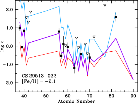
Figure 18.— Derived neutron-capture abundances in CS 29513–032. Symbols are the same as in Figure 13. The red curve indicates the $r$-process standard star CS 22892–052, the blue curve indicates the Solar metallicity $s$-process predictions of Arlandini et al. (1999), and the bold purple curve indicates a linear combination of the two other curves that approximately matches the derived 1^st peak and rare earth abundances. All curves are normalized to the derived Eu abundance.

We find two extremely metal-poor stars ([Fe/H] $=-3.3$ and $-3.4$) in the stream, suggesting that whatever progenitor produced the stream was capable of producing extremely metal-poor stars like those observed in the stellar halo and a handful of dwarf galaxies. The stream stars span a range of metallicities, unlike individual Galactic globular clusters, which have no significant internal metallicity spread. The stream also exhibits smaller star-to-star chemical dispersion than the Milky Way dwarf galaxies. We cannot identify a direct progenitor of the stream, but our results support the notion that a significant fraction of the Milky Way stellar halo can form from accreted systems.

Appendix A CS 29513–032

CS 29513–032 shows clear enrichment by the $s$-process, with large overabundances of [C/Fe] $=+0.6$ and [Pb/Fe] $=+1.8$. The Ba is also enhanced, with [Ba/Fe] $=+0.8$ and [Ba/Eu] $=+0.4$. In contrast, the other stream members—enriched by the $r$-process—have $\langle$[Ba/Eu]$\rangle=-0.35$ ($\sigma=0.13$). Low-metallicity stars on the AGB (or stars polluted by their nucleosynthetic products) are also predicted to be Na-enhanced, which has been observationally confirmed (e.g., Ivans et al. 2005; Roederer et al. 2008). CS 29513–032 is also Na-enhanced, with [Na/Fe] $\approx+0.15$ (approximately corrected for NLTE; e.g., Andrievsky et al. 2007). The $n$-capture enrichment pattern of CS 29513–032 is illustrated in Figure 18. In contrast to the weak and main $r$-process enrichment seen in Figure 12, the Pb abundance lies far above the Pb abundance predicted from the Pb/Eu $r$-process ratio.

We can approximately fit the observed abundance pattern in CS 29513–032 by taking linear combinations of the $s$- and $r$-process template abundance patterns, as indicated by the bold curve in Figure 18. This predicted distribution (normalized to the Eu abundance) provides a reasonable fit to the 1^st peak and rare earth elements in CS 29513–032. The derived Pb abundance is still higher than the predicted Pb abundance because the prediction is based on a Solar-metallicity AGB model. According to the observed and predicted [Pb/Ba] ratios for a 1.5 $M_{\odot}$ AGB model presented in Figure 20 of Sneden et al. (2008), one might expect a [Pb/Ba] ratio of $\sim+1.0$ ($\pm\sim 0.5$) at [Fe/H] $=-2.0$. This translates to [Pb_[Fe/H]=-2/Pb_[Fe/H]=0] $\sim+1.0$. Indeed, the derived Pb abundance in CS 29513–032 is roughly 1 dex higher than the predicted Pb abundance based on the Solar $s$-process model. Even in the absence of detailed calculations, the high [Pb/Fe] ratio in CS 29513–032 clearly indicates an $s$-process origin.

CS 29513–032 is a subgiant and has not passed through the AGB phase of evolution where the $s$-process is expected to occur. We speculate that the $s$-process material observed in this star was produced in another low-metallicity star in the AGB phase, likely a binary companion that has long since faded from view.

Table 1Log of Observations

Star	Telescope/	Exp.	Date	UT mid-	Heliocentric	Heliocentric
	Instrument	time (s)		exposure	JD	RV (km s-1)
BD$+$10 2495	McDonald-Smith/2dCoude	5600	2009 May 06	06:23	2454957.771	$+$250.8
BD$+$10 2495	McDonald-Smith/2dCoude	3600	2009 Jun 10	04:31	2454992.690	$+$250.8
BD$+$29 2356	McDonald-Smith/2dCoude	5400	2009 Jun 11	05:45	2454993.741	$-$207.3
BD$+$30 2611	McDonald-Smith/2dCoude	2700	2009 May 06	07:43	2454957.826	$-$280.4
BD$+$30 2611	McDonald-Smith/2dCoude	2300	2009 Jun 10	05:25	2454992.729	$-$280.0
BD$+$30 2611	McDonald-Smith/2dCoude	2500	2009 Jun 14	07:28	2454996.814	$-$280.4
CD$-$36 1052	Magellan-Clay/MIKE	1200	2009 Jul 04	10:12	2455016.924	$+$304.7
CS 22876–040	Magellan-Clay/MIKE	5800	2009 Jul 26	07:17	2455038.807	$-$189.9
CS 22948–093	Magellan-Clay/MIKE	1400	2006 Aug 03	04:07	2453950.677	$+$367.9
CS 22948–093	Magellan-Clay/MIKE	900	2009 Oct 26	02:42	2455130.614	$+$360.4
CS 29513–031	Magellan-Clay/MIKE	5400	2006 Jul 19	09:11	2453935.887	$+$295.7
CS 29513–031	Magellan-Clay/MIKE	1200	2009 Jul 04	09:44	2455016.909	$+$283.8
CS 29513–031	Magellan-Clay/MIKE	1200	2009 Jul 25	06:14	2455037.764	$+$283.6
CS 29513–031	Magellan-Clay/MIKE	1200	2009 Oct 28	01:58	2455132.584	$+$284.1
CS 29513–032	Magellan-Clay/MIKE	3800	2009 Jul 25	09:04	2455037.882	$-$215.8
CS 29513–032	Magellan-Clay/MIKE	600	2009 Oct 26	03:27	2455130.646	$-$215.4
HD 119516	McDonald-Smith/2dCoude	2700	2009 May 07	06:40	2454958.782	$-$285.9
HD 128279	Magellan-Clay/MIKE	200	2004 Jul 14	22:49	2453201.453	$-$75.7
HD 128279	Magellan-Clay/MIKE	20	2004 Jun 22	22:57	2453179.460	$-$76.1
HD 128279	Magellan-Clay/MIKE	90	2004 Jul 23	22:59	2453210.459	$-$75.7
HD 128279	Magellan-Clay/MIKE	240	2005 May 31	03:05	2453521.634	$-$75.3
HD 175305	McDonald-Smith/2dCoude	1500	2009 May 06	11:14	2454957.967	$-$184.2
HD 237846	McDonald-Smith/2dCoude	6000	2009 Jun 11	03:30	2454993.643	$-$303.8
HD 237846	McDonald-Smith/2dCoude	2100	2009 Jun 14	02:58	2454996.620	$-$303.5

Table 2Observational Stellar Data

Star	$\alpha$	$\delta$	$\langle$RV$\rangle$	Binary	Total exp.	No.	S/N	S/N	S/N	S/N
	(J2000)	(J2000)	(km s-1)	flag	time (s)	obs.	3950Å	4550Å	5200Å	6750Å
BD$+$10 2495	12:59:20	$+$09:14:36	$+$258.3	3	9200	2	50	105	140	185
BD$+$29 2356	13:01:52	$+$29:11:18	$-$207.3	1	5400	1	20	50	65	85
BD$+$30 2611	15:06:54	$+$30:00:37	$-$280.3	1	7500	3	35	120	180	270
CD$-$36 1052	02:47:38	$-$36:06:24	$+$304.7	1	1200	1	85	140	130	195
CS 22876–040	00:04:52	$-$34:13:37	$-$189.9	0	5800	1	60	100	90	135
CS 22948–093	21:50:32	$-$41:07:49	$\cdots$	2	10300	4	85	110	75	95
CS 29513–031	23:25:11	$-$39:59:29	$\cdots$	2	7800	3	80	105	80	100
CS 29513–032	23:22:19	$-$39:44:25	$-$215.6	1	4400	2	60	100	95	140
HD 119516	13:43:27	$+$15:34:31	$-$285.9	1	2700	1	65	120	150	175
HD 128279	14:36:50	$-$29:06:46	$-$75.7	1	550	4	625	880	505	750
HD 175305	18:47:06	$+$74:43:31	$-$184.2	1	1500	1	60	135	190	250
HD 237846	09:52:39	$+$57:54:59	$-$303.6	1	8100	2	45	100	135	185

Table 3References for Transition Probabilities or Oscillator Strengths

Species	Reference(s) and Comments
Li i	Yan et al. (1998)
C	CH $A^{2}\Delta-X^{2}\Pi$ G-band linelist from B. Plez (private communication)
N	CN $B^{2}\Sigma-X^{2}\Sigma$ (0,0) band from Kurucz & Bell (1995)
O i	Fuhr & Wiese (2009)
Na i	Fuhr & Wiese (2009)
Mg i	Aldenius et al. (2007) for the Mg b triplet; Barklem et al. (2005)
	and references therein for all other transitions
Al i	Fuhr & Wiese (2009)
Si i	Fuhr & Wiese (2009), Nahar & Pradhan (1993), via NIST
K i	Fuhr & Wiese (2009)
Ca i	Fuhr & Wiese (2009)
Sc ii	Lawler & Dakin (1989)
Ti i	Blackwell et al. (1982a, b), increased by 0.056 dex
	according to Grevesse et al. (1989)
Ti ii	Pickering et al. (2001) (with corrections given in Pickering et al. (2002))
V i	Doerr et al. (1985)
V ii	Biémont et al. (1989)
Cr i	Sobeck et al. (2007)
Cr ii	Nilsson et al. (2006)
Mn i	Booth et al. (1984), Blackwell-Whitehead & Bergemann (2007)
Mn ii	Martinson et al. (1977)
Fe i	O’Brian et al. (1991)
Fe ii	Meléndez & Barbuy (2009)
Co i	Nitz et al. (1999), otherwise Cardon et al. (1982)
Ni i	Blackwell et al. (1989), otherwise Doerr & Kock (1985)
Cu i	Fuhr & Wiese (2009)
Zn i	Biémont & Godefroid (1980)
Rb i	Fuhr & Wiese (2009)
Sr ii	Fuhr & Wiese (2009)
Y ii	Hannaford et al. (1982)
Zr ii	Biémont et al. (1981)
Nb ii	Hannaford et al. (1985)
Mo i	Whaling & Brault (1988)
Ru i	Wickliffe et al. (1994)
Ba ii	Fuhr & Wiese (2009)
La ii	Lawler et al. (2001a)
Ce ii	Lawler et al. (2009)
Pr ii	Ivarsson et al. (2001), Li et al. (2007)
Nd ii	Den Hartog et al. (2003)
Sm ii	Lawler et al. (2006)
Eu ii	Lawler et al. (2001b)
Gd ii	Den Hartog et al. (2006)
Tb ii	Lawler et al. (2001c)
Dy ii	Wickliffe et al. (2000)
Ho ii	Lawler et al. (2004)
Er ii	Lawler et al. (2008)
Tm ii	Wickliffe & Lawler (1997)
Yb ii	Biémont et al. (1998), renormalized to Pinnington et al. (1997);
	see the appendix of Sneden et al. (2009) for discussion
Hf ii	Lawler et al. (2007)
Ir ii	Ivarsson et al. (2003)
Pb ii	Biémont et al. (2000)
Th ii	Nilsson et al. (2002)

Table 4Equivalent Width Measurements for All Stars

Wavelength (Å)	Species ID	E.P. (eV)	$\log(gf)$	E.W. (mÅ)
BD$+$10 2495
6707.80	3.0	0.00	0.17	synth
6300.30	8.0	0.00	-9.78	$\cdots$
7771.94	8.0	9.14	0.37	7.1
7774.17	8.0	9.14	0.22	7.5
7775.39	8.0	9.14	0.00	5.2
⋮	⋮	⋮	⋮	⋮

Note. — The full table is available in machine-readable form in the electronic edition of the journal; only a small portion is shown here to present its general form and content.

Table 5Model Atmosphere Parameters

Star	Teff	log $g$	$v_{t}$	[M/H]	Evolutionary
	(K)		(km s-1)		state
BD$+$10 2495	4710	1.30	1.55	$-$2.45	RGB
BD$+$29 2356	4760	1.60	1.45	$-$1.55	RGB
BD$+$30 2611	4330	0.60	1.85	$-$1.45	RGB
CD$-$36 1052	6070	2.30	3.20	$-$1.65	RHB
CS 22876–040	6280	3.70	1.60	$-$2.30	SGB
CS 22948–093	6480	4.00	1.15	$-$3.35	SGB
CS 29513–031	6650	3.70	0.80	$-$2.55	SGB
CS 29513–032	5810	3.30	1.45	$-$2.10	SGB
HD 119516	5290	1.10	2.25	$-$2.15	RHB
HD 128279	5050	2.35	1.50	$-$2.45	RGB
HD 175305	4770	1.80	1.25	$-$1.60	RGB
HD 237846	4600	1.00	1.50	$-$3.20	RGB

Table 6Comparison of Temperature Estimates

Star	$T_{\rm eff}$	$T_{\rm eff}(V-J)$	$T_{\rm eff}(V-H)$	$T_{\rm eff}(V-K)$	$\Delta T_{\rm mean}$
	(K)	(K)	(K)	(K)	(K)
BD$+$10 2495	4710	4946$\pm$119	4916$\pm$69	4964$\pm$74	$-$232
BD$+$30 2611	4330	4258$\pm$209	4141$\pm$78	4244$\pm$40	$+$116
HD 128279	5050	5274$\pm$157	5282$\pm$94	5305$\pm$82	$-$237
HD 175305	4770	5063$\pm$152	5028$\pm$85	5042$\pm$66	$-$274
HD 237846	4600	4968$\pm$123	4984$\pm$85	4985$\pm$65	$-$379

Table 7Elemental Abundances I. 

	BD$+$10 2495					BD$+$29 2356					BD$+$30 2611
Species	log $\epsilon$(X)	[X/Fe]	$\sigma$	Nlines		log($\epsilon$)	[X/Fe]	$\sigma$	Nlines		log($\epsilon$)	[X/Fe]	$\sigma$	Nlines
	(dex)	(dex)	(dex)			(dex)	(dex)	(dex)			(dex)	(dex)	(dex)
Li I	0.57	-1.63	0.25	1		$<$ 0.70	$\cdots$	$\cdots$	$\cdots$		$<$ -0.01	$\cdots$	$\cdots$	$\cdots$
C	5.92	-0.31	0.20	1		6.71	-0.24	0.20	1		6.32	-0.72	0.30	1
N	$\cdots$	$\cdots$	$\cdots$	$\cdots$		6.57	0.36	0.20	1		$\cdots$	$\cdots$	$\cdots$	$\cdots$
O I	7.30	0.70	0.11	3		8.04	0.72	0.25	1		7.40	-0.01	0.30	1
Na I	3.89	-0.11	0.25	1		4.51	-0.21	0.15	2		4.55	-0.26	0.15	2
Mg I	5.78	0.53	0.15	4		6.34	0.37	0.11	3		6.37	0.31	0.16	3
Al I	3.56	-0.58	0.25	1		$\cdots$	$\cdots$	$\cdots$	$\cdots$		$\cdots$	$\cdots$	$\cdots$	$\cdots$
Si I	5.72	0.50	0.15	2		6.10	0.16	0.23	4		6.12	0.09	0.18	3
K I	$\cdots$	$\cdots$	$\cdots$	$\cdots$		4.28	0.77	0.25	1		4.14	0.54	0.25	1
Ca I	4.46	0.43	0.10	9		5.20	0.45	0.10	7		5.13	0.29	0.10	5
Sc II	0.63	-0.14	0.11	6		1.63	0.14	0.10	5		1.47	-0.11	0.25	1
Ti I	2.72	0.06	0.10	16		3.48	0.10	0.10	14		3.41	-0.06	0.10	9
Ti II	2.81	0.15	0.10	20		3.74	0.36	0.12	12		3.61	0.14	0.11	5
V I	1.36	-0.31	0.25	1		1.88	-0.51	0.25	1		$\cdots$	$\cdots$	$\cdots$	$\cdots$
V II	1.62	-0.05	0.16	2		2.36	-0.03	0.30	1		$\cdots$	$\cdots$	$\cdots$	$\cdots$
Cr I	3.11	-0.23	0.10	10		3.94	-0.12	0.10	9		4.02	-0.13	0.10	4
Cr II	3.54	0.20	0.10	3		4.16	0.10	0.25	1		$\cdots$	$\cdots$	$\cdots$	$\cdots$
Mn I	2.72	-0.34	0.18	8		3.44	-0.34	0.10	5		3.52	-0.35	0.25	1
Mn II	$\cdots$	$\cdots$	$\cdots$	$\cdots$		$\cdots$	$\cdots$	$\cdots$	$\cdots$		$\cdots$	$\cdots$	$\cdots$	$\cdots$
Fe I	5.19	0.00	0.10	112		5.91	0.00	0.11	82		6.00	0.00	0.10	58
Fe II	5.13	-0.06	0.10	9		5.81	-0.10	0.10	7		5.97	-0.03	0.10	10
Co I	2.46	-0.13	0.15	2		3.18	-0.13	0.25	1		$\cdots$	$\cdots$	$\cdots$	$\cdots$
Ni I	3.91	-0.01	0.10	8		4.65	0.01	0.18	7		4.70	-0.03	0.17	4
Cu I	0.99	-0.89	0.25	1		2.05	-0.55	0.25	1		$\cdots$	$\cdots$	$\cdots$	$\cdots$
Zn I	2.32	0.05	0.25	1		3.05	0.06	0.15	2		2.87	-0.21	0.15	2
Rb I	$\cdots$	$\cdots$	$\cdots$	$\cdots$		$<$ 2.00	$<$ 1.09	$\cdots$	$\cdots$		$<$ 1.25	$<$ 0.25	$\cdots$	$\cdots$
Sr II	0.44	-0.08	0.30	1		1.26	0.02	0.30	2		1.00	-0.33	0.25	1
Y II	-0.52	-0.43	0.10	4		0.52	-0.11	0.10	3		0.41	-0.31	0.10	3
Zr II	0.27	0.00	0.10	3		1.33	0.34	0.10	3		1.08	0.01	0.15	2
Nb II	$<$ 0.59	$<$ 1.46	$\cdots$	$\cdots$		$<$ 1.63	$<$ 1.78	$\cdots$	$\cdots$		$\cdots$	$\cdots$	$\cdots$	$\cdots$
Mo I	-0.43	0.02	0.25	1		0.46	0.19	0.25	1		0.38	0.02	0.30	1
Tc I	$<$ 0.29	$<$ 2.62	$\cdots$	$\cdots$		$<$ 1.08	$<$ 2.69	$\cdots$	$\cdots$		$\cdots$	$\cdots$	$\cdots$	$\cdots$
Ru I	$\cdots$	$\cdots$	$\cdots$	$\cdots$		$\cdots$	$\cdots$	$\cdots$	$\cdots$		$\cdots$	$\cdots$	$\cdots$	$\cdots$
Ba II	-0.38	-0.01	0.18	2		0.62	0.09	0.15	2		0.68	0.06	0.25	1
La II	-1.36	-0.22	0.10	4		-0.47	-0.05	0.10	4		-0.24	0.09	0.13	9
Ce II	-0.97	-0.07	0.10	4		-0.06	0.12	0.13	4		0.14	0.23	0.10	7
Pr II	-1.17	0.35	0.25	1		-0.45	0.31	0.16	3		-0.50	0.17	0.16	5
Nd II	-0.92	-0.06	0.10	5		0.16	0.30	0.16	6		0.26	0.31	0.10	7
Sm II	-1.28	0.09	0.15	2		-0.31	0.34	0.15	2		-0.12	0.44	0.10	7
Eu II	-1.69	0.13	0.10	3		-0.69	0.41	0.25	1		-0.36	0.65	0.15	2
Gd II	-1.07	0.18	0.15	2		-0.07	0.46	0.22	2		0.20	0.64	0.21	3
Tb II	-1.77	0.21	0.30	1		-0.94	0.32	0.25	1		-0.86	0.31	0.25	1
Dy II	-1.05	0.22	0.10	4		0.04	0.59	0.21	2		0.38	0.84	0.17	3
Ho II	-1.80	0.06	0.30	1		-0.64	0.50	0.30	1		$\cdots$	$\cdots$	$\cdots$	$\cdots$
Er II	-1.20	0.21	0.15	2		0.04	0.73	0.30	1		$\cdots$	$\cdots$	$\cdots$	$\cdots$
Tm II	-2.16	-0.06	0.30	1		$\cdots$	$\cdots$	$\cdots$	$\cdots$		$\cdots$	$\cdots$	$\cdots$	$\cdots$
Yb II	-1.25	0.17	0.25	1		-0.28	0.44	0.30	1		$\cdots$	$\cdots$	$\cdots$	$\cdots$
Hf II	$<$ -1.30	$<$ 0.19	$\cdots$	$\cdots$		-0.54	0.22	0.30	1		-0.46	0.21	0.15	2
Ir I	$<$ -0.11	$<$ 0.87	$\cdots$	$\cdots$		$<$ 1.04	$<$ 1.30	$\cdots$	$\cdots$		0.35	0.52	0.35	1
Pb I	$<$ 0.88	$<$ 1.32	$\cdots$	$\cdots$		0.35	0.07	0.30	1		0.56	0.19	0.30	1
Th II	-1.96	0.25	0.30	1		-1.07	0.42	0.30	1		-0.98	0.42	0.30	1

Table 8Elemental Abundances II. 

	CD$-$36 1052					CS 22876–040					CS 22948–093
Species	log $\epsilon$(X)	[X/Fe]	$\sigma$	Nlines		log($\epsilon$)	[X/Fe]	$\sigma$	Nlines		log($\epsilon$)	[X/Fe]	$\sigma$	Nlines
	(dex)	(dex)	(dex)			(dex)	(dex)	(dex)			(dex)	(dex)	(dex)
Li I	$<$ 1.79	$\cdots$	$\cdots$	$\cdots$		2.09	-0.11	0.25	1		$<$ 2.35	$\cdots$	$\cdots$	$\cdots$
C	$<$ 7.05	$<$ 0.30	$\cdots$	$\cdots$		$<$ 6.79	$<$ 0.59	$\cdots$	$\cdots$		$<$ 6.90	$<$ 1.72	$\cdots$	$\cdots$
N	$<$ 8.80	$<$ 2.79	$\cdots$	$\cdots$		$<$ 8.50	$<$ 3.04	$\cdots$	$\cdots$		$<$ 8.60	$<$ 4.16	$\cdots$	$\cdots$
O I	7.94	0.82	0.12	3		7.20	0.63	0.10	3		$<$ 7.23	$<$ 1.68	$\cdots$	$\cdots$
Na I	$\cdots$	$\cdots$	$\cdots$	$\cdots$		$\cdots$	$\cdots$	$\cdots$	$\cdots$		$<$ 2.27	$<$ -0.68	$\cdots$	$\cdots$
Mg I	6.13	0.36	0.10	5		5.53	0.31	0.10	4		4.44	0.24	0.15	3
Al I	3.90	-0.76	0.15	2		3.25	-0.86	0.25	1		2.40	-0.69	0.15	2
Si I	6.06	0.32	0.25	1		5.56	0.37	0.25	1		4.15	-0.02	0.25	1
K I	3.77	0.46	0.25	1		$\cdots$	$\cdots$	$\cdots$	$\cdots$		$\cdots$	$\cdots$	$\cdots$	$\cdots$
Ca I	4.88	0.33	0.10	12		4.50	0.50	0.10	13		3.43	0.45	0.10	3
Sc II	1.55	0.24	0.14	7		0.88	0.14	0.10	3		0.18	0.46	0.10	4
Ti I	3.37	0.19	0.10	7		3.17	0.54	0.11	7		$\cdots$	$\cdots$	$\cdots$	$\cdots$
Ti II	3.48	0.30	0.10	16		3.07	0.44	0.10	21		2.03	0.42	0.10	7
V I	2.23	0.04	0.25	1		$\cdots$	$\cdots$	$\cdots$	$\cdots$		$\cdots$	$\cdots$	$\cdots$	$\cdots$
V II	2.38	0.19	0.25	1		1.81	0.17	0.15	2		$<$ 1.87	$<$ 1.25	$\cdots$	$\cdots$
Cr I	3.76	-0.10	0.12	7		3.19	-0.12	0.10	3		2.07	-0.22	0.15	2
Cr II	4.08	0.22	0.10	3		3.54	0.23	0.15	2		$\cdots$	$\cdots$	$\cdots$	$\cdots$
Mn I	3.38	-0.20	0.15	5		2.70	-0.33	0.10	3		1.91	-0.10	0.30	1
Mn II	$\cdots$	$\cdots$	$\cdots$	$\cdots$		$\cdots$	$\cdots$	$\cdots$	$\cdots$		$\cdots$	$\cdots$	$\cdots$	$\cdots$
Fe I	5.71	0.00	0.10	107		5.16	0.00	0.10	107		4.14	0.00	0.11	37
Fe II	5.76	0.05	0.10	8		5.27	0.11	0.10	10		4.12	-0.02	0.25	1
Co I	3.16	0.05	0.25	1		2.54	-0.02	0.12	3		$\cdots$	$\cdots$	$\cdots$	$\cdots$
Ni I	4.32	-0.12	0.10	4		3.93	0.04	0.11	5		2.90	0.03	0.22	3
Cu I	$\cdots$	$\cdots$	$\cdots$	$\cdots$		$\cdots$	$\cdots$	$\cdots$	$\cdots$		$\cdots$	$\cdots$	$\cdots$	$\cdots$
Zn I	2.88	0.09	0.15	2		2.38	0.14	0.15	2		$<$ 2.35	$<$ 1.13	$\cdots$	$\cdots$
Rb I	$<$ 3.08	$<$ 2.37	$\cdots$	$\cdots$		$\cdots$	$\cdots$	$\cdots$	$\cdots$		$\cdots$	$\cdots$	$\cdots$	$\cdots$
Sr II	1.57	0.53	0.15	2		0.70	0.21	0.15	2		-0.40	0.08	0.15	2
Y II	0.34	-0.09	0.10	4		0.12	0.24	0.15	2		$<$ -0.64	$<$ 0.50	$\cdots$	$\cdots$
Zr II	1.11	0.32	0.13	3		0.86	0.62	0.24	2		$<$ 0.37	$<$ 1.15	$\cdots$	$\cdots$
Nb II	$<$ 1.27	$<$ 1.62	$\cdots$	$\cdots$		$\cdots$	$\cdots$	$\cdots$	$\cdots$		$<$ 1.61	$<$ 3.57	$\cdots$	$\cdots$
Mo I	$<$ 1.73	$<$ 1.66	$\cdots$	$\cdots$		$<$ 1.82	$<$ 2.30	$\cdots$	$\cdots$		$<$ 1.40	$<$ 2.86	$\cdots$	$\cdots$
Tc I	$<$ 2.09	$<$ 3.90	$\cdots$	$\cdots$		$<$ 2.03	$<$ 4.39	$\cdots$	$\cdots$		$<$ 1.83	$<$ 5.21	$\cdots$	$\cdots$
Ru I	$\cdots$	$\cdots$	$\cdots$	$\cdots$		$\cdots$	$\cdots$	$\cdots$	$\cdots$		$\cdots$	$\cdots$	$\cdots$	$\cdots$
Ba II	0.46	0.13	0.15	2		-0.10	0.12	0.11	3		-0.88	0.37	0.15	2
La II	-0.40	0.22	0.10	3		$<$ -0.09	$<$ 1.08	$\cdots$	$\cdots$		$\cdots$	$\cdots$	$\cdots$	$\cdots$
Ce II	$<$ 0.15	$<$ 0.53	$\cdots$	$\cdots$		$<$ 0.50	$<$ 1.21	$\cdots$	$\cdots$		$<$ 0.43	$<$ 2.26	$\cdots$	$\cdots$
Pr II	$<$ 0.12	$<$ 1.08	$\cdots$	$\cdots$		$<$ 0.50	$<$ 2.01	$\cdots$	$\cdots$		$<$ 0.02	$<$ 2.69	$\cdots$	$\cdots$
Nd II	0.04	0.30	0.15	2		$<$ 0.29	$<$ 1.18	$\cdots$	$\cdots$		$<$ 0.06	$<$ 1.94	$\cdots$	$\cdots$
Sm II	-0.37	0.48	0.30	1		$<$ 0.26	$<$ 1.66	$\cdots$	$\cdots$		$<$ 0.19	$<$ 2.57	$\cdots$	$\cdots$
Eu II	-0.82	0.48	0.10	3		$<$ -0.70	$<$ 1.15	$\cdots$	$\cdots$		$<$ -0.96	$<$ 1.91	$\cdots$	$\cdots$
Gd II	$<$ 0.36	$<$ 1.09	$\cdots$	$\cdots$		$<$ 0.73	$<$ 2.01	$\cdots$	$\cdots$		$<$ 0.46	$<$ 2.72	$\cdots$	$\cdots$
Tb II	$<$ -0.12	$<$ 1.34	$\cdots$	$\cdots$		$<$ 0.26	$<$ 2.27	$\cdots$	$\cdots$		$<$ -0.06	$<$ 2.99	$\cdots$	$\cdots$
Dy II	-0.30	0.45	0.25	1		$<$ 0.08	$<$ 1.38	$\cdots$	$\cdots$		$<$ 0.51	$<$ 2.79	$\cdots$	$\cdots$
Ho II	$\cdots$	$\cdots$	$\cdots$	$\cdots$		$<$ 0.41	$<$ 2.30	$\cdots$	$\cdots$		$<$ -0.25	$<$ 2.63	$\cdots$	$\cdots$
Er II	$<$ 0.10	$<$ 0.99	$\cdots$	$\cdots$		$<$ 0.30	$<$ 1.74	$\cdots$	$\cdots$		$<$ 0.07	$<$ 2.52	$\cdots$	$\cdots$
Tm II	$<$ -0.29	$<$ 1.29	$\cdots$	$\cdots$		$<$ -0.03	$<$ 2.10	$\cdots$	$\cdots$		$\cdots$	$\cdots$	$\cdots$	$\cdots$
Yb II	-0.63	0.22	0.30	1		$\cdots$	$\cdots$	$\cdots$	$\cdots$		$\cdots$	$\cdots$	$\cdots$	$\cdots$
Hf II	$<$ 0.63	$<$ 1.59	$\cdots$	$\cdots$		$<$ 0.89	$<$ 2.40	$\cdots$	$\cdots$		$<$ 0.87	$<$ 3.37	$\cdots$	$\cdots$
Ir I	$\cdots$	$\cdots$	$\cdots$	$\cdots$		$<$ 2.46	$<$ 3.47	$\cdots$	$\cdots$		$\cdots$	$\cdots$	$\cdots$	$\cdots$
Pb I	$<$ 2.47	$<$ 2.39	$\cdots$	$\cdots$		$<$ 2.14	$<$ 2.61	$\cdots$	$\cdots$		$<$ 1.85	$<$ 3.38	$\cdots$	$\cdots$
Th II	$\cdots$	$\cdots$	$\cdots$	$\cdots$		$\cdots$	$\cdots$	$\cdots$	$\cdots$		$<$ 0.13	$<$ 3.39	$\cdots$	$\cdots$

Table 9Elemental Abundances III. 

	CS 29513–031					CS 29513–032					HD 119516
Species	log $\epsilon$(X)	[X/Fe]	$\sigma$	Nlines		log($\epsilon$)	[X/Fe]	$\sigma$	Nlines		log($\epsilon$)	[X/Fe]	$\sigma$	Nlines
	(dex)	(dex)	(dex)			(dex)	(dex)	(dex)			(dex)	(dex)	(dex)
Li I	$<$ 2.50	$\cdots$	$\cdots$	$\cdots$		2.16	-0.04	0.25	1		$<$ 1.14	$\cdots$	$\cdots$	$\cdots$
C	$<$ 7.10	$<$ 1.20	$\cdots$	$\cdots$		7.09	0.63	0.20	1		$<$ 5.86	$<$ -0.42	$\cdots$	$\cdots$
N	$<$ 8.60	$<$ 3.19	$\cdots$	$\cdots$		$<$ 6.90	$<$ 1.04	$\cdots$	$\cdots$		$<$ 7.80	$<$ 2.26	$\cdots$	$\cdots$
O I	6.82	0.55	0.20	3		7.48	0.65	0.10	3		7.26	0.61	0.10	3
Na I	4.49	0.82	0.25	1		4.69	0.46	0.25	1		3.79	-0.26	0.25	1
Mg I	5.24	0.32	0.10	3		6.00	0.52	0.14	5		5.64	0.34	0.10	5
Al I	2.96	-0.85	0.30	1		3.90	-0.49	0.22	2		3.22	-0.97	0.16	2
Si I	4.92	0.03	0.25	1		6.11	0.66	0.25	1		5.81	0.54	0.25	1
K I	$\cdots$	$\cdots$	$\cdots$	$\cdots$		3.50	0.48	0.25	1		3.17	0.33	0.15	2
Ca I	4.11	0.41	0.12	6		4.71	0.45	0.10	12		4.41	0.33	0.10	9
Sc II	0.48	0.04	0.30	1		0.91	-0.09	0.10	4		0.73	-0.09	0.13	6
Ti I	$\cdots$	$\cdots$	$\cdots$	$\cdots$		3.09	0.20	0.10	11		2.84	0.13	0.10	16
Ti II	2.51	0.18	0.10	6		3.04	0.15	0.10	19		2.69	-0.02	0.11	20
V I	$\cdots$	$\cdots$	$\cdots$	$\cdots$		1.95	0.05	0.25	1		1.58	-0.14	0.25	1
V II	$\cdots$	$\cdots$	$\cdots$	$\cdots$		1.78	-0.12	0.15	2		1.60	-0.12	0.15	2
Cr I	2.88	-0.13	0.15	2		3.45	-0.12	0.12	7		3.24	-0.15	0.10	10
Cr II	$\cdots$	$\cdots$	$\cdots$	$\cdots$		3.69	0.12	0.11	3		3.56	0.17	0.10	3
Mn I	2.61	-0.12	0.20	2		3.03	-0.26	0.13	6		2.78	-0.33	0.17	6
Mn II	$\cdots$	$\cdots$	$\cdots$	$\cdots$		$\cdots$	$\cdots$	$\cdots$	$\cdots$		$\cdots$	$\cdots$	$\cdots$	$\cdots$
Fe I	4.86	0.00	0.10	48		5.42	0.00	0.10	118		5.24	0.00	0.10	114
Fe II	4.82	-0.04	0.10	4		5.34	-0.08	0.10	11		5.19	-0.05	0.10	10
Co I	$\cdots$	$\cdots$	$\cdots$	$\cdots$		2.80	-0.02	0.11	4		2.52	-0.12	0.10	3
Ni I	3.73	0.14	0.33	3		4.15	0.00	0.13	8		3.92	-0.05	0.10	6
Cu I	$\cdots$	$\cdots$	$\cdots$	$\cdots$		2.08	-0.03	0.25	1		$\cdots$	$\cdots$	$\cdots$	$\cdots$
Zn I	$<$ 2.72	$<$ 0.78	$\cdots$	$\cdots$		2.61	0.11	0.15	2		2.32	0.00	0.15	2
Rb I	$\cdots$	$\cdots$	$\cdots$	$\cdots$		$<$ 2.97	$<$ 2.55	$\cdots$	$\cdots$		$<$ 2.72	$<$ 2.48	$\cdots$	$\cdots$
Sr II	-0.20	-0.44	0.20	2		1.00	0.25	0.15	2		0.83	0.26	0.15	2
Y II	$<$ -0.32	$<$ 0.10	$\cdots$	$\cdots$		-0.06	-0.20	0.10	3		-0.43	-0.39	0.10	4
Zr II	$<$ 1.08	$<$ 1.14	$\cdots$	$\cdots$		0.83	0.33	0.12	3		0.29	-0.03	0.10	3
Nb II	$\cdots$	$\cdots$	$\cdots$	$\cdots$		$<$ 1.57	$<$ 2.21	$\cdots$	$\cdots$		$<$ 0.26	$<$ 1.08	$\cdots$	$\cdots$
Mo I	$<$ 1.77	$<$ 2.51	$\cdots$	$\cdots$		$<$ 1.33	$<$ 1.55	$\cdots$	$\cdots$		$<$ 0.31	$<$ 0.71	$\cdots$	$\cdots$
Tc I	$<$ 1.96	$<$ 4.62	$\cdots$	$\cdots$		$<$ 1.88	$<$ 3.98	$\cdots$	$\cdots$		$<$ 0.97	$<$ 3.25	$\cdots$	$\cdots$
Ru I	$\cdots$	$\cdots$	$\cdots$	$\cdots$		$\cdots$	$\cdots$	$\cdots$	$\cdots$		$\cdots$	$\cdots$	$\cdots$	$\cdots$
Ba II	-0.84	-0.31	0.30	1		0.80	0.76	0.17	4		-0.16	-0.02	0.24	2
La II	$\cdots$	$\cdots$	$\cdots$	$\cdots$		-0.52	0.39	0.17	4		-1.08	0.01	0.10	4
Ce II	$<$ 0.43	$<$ 1.54	$\cdots$	$\cdots$		0.12	0.79	0.43	2		-0.64	0.21	0.11	3
Pr II	$<$ 0.19	$<$ 2.14	$\cdots$	$\cdots$		$<$ 0.04	$<$ 1.26	$\cdots$	$\cdots$		-1.23	0.20	0.22	3
Nd II	$<$ 0.11	$<$ 1.27	$\cdots$	$\cdots$		-0.05	0.58	0.25	1		-0.74	0.07	0.10	6
Sm II	$<$ 0.23	$<$ 1.89	$\cdots$	$\cdots$		$\cdots$	$\cdots$	$\cdots$	$\cdots$		-1.11	0.21	0.15	2
Eu II	$<$ -1.01	$<$ 1.14	$\cdots$	$\cdots$		-1.20	0.39	0.29	2		-1.43	0.34	0.10	3
Gd II	$<$ 0.48	$<$ 2.02	$\cdots$	$\cdots$		$<$ 0.46	$<$ 1.48	$\cdots$	$\cdots$		-0.76	0.44	0.10	3
Tb II	$<$ 0.06	$<$ 2.39	$\cdots$	$\cdots$		$<$ -0.07	$<$ 1.68	$\cdots$	$\cdots$		$\cdots$	$\cdots$	$\cdots$	$\cdots$
Dy II	$<$ -0.17	$<$ 1.39	$\cdots$	$\cdots$		-0.43	0.61	0.35	1		-0.77	0.45	0.25	1
Ho II	$\cdots$	$\cdots$	$\cdots$	$\cdots$		$\cdots$	$\cdots$	$\cdots$	$\cdots$		$\cdots$	$\cdots$	$\cdots$	$\cdots$
Er II	$<$ 0.13	$<$ 1.86	$\cdots$	$\cdots$		$<$ 0.12	$<$ 1.30	$\cdots$	$\cdots$		-1.02	0.34	0.15	2
Tm II	$<$ -0.29	$<$ 2.24	$\cdots$	$\cdots$		$<$ -0.40	$<$ 1.47	$\cdots$	$\cdots$		-1.83	0.22	0.25	1
Yb II	$\cdots$	$\cdots$	$\cdots$	$\cdots$		-0.62	0.58	0.25	1		-1.21	0.15	0.35	1
Hf II	$<$ 0.88	$<$ 2.66	$\cdots$	$\cdots$		$<$ 0.52	$<$ 1.77	$\cdots$	$\cdots$		-1.21	0.22	0.40	1
Ir I	$\cdots$	$\cdots$	$\cdots$	$\cdots$		$<$ 2.25	$<$ 3.00	$\cdots$	$\cdots$		$\cdots$	$\cdots$	$\cdots$	$\cdots$
Pb I	$<$ 2.17	$<$ 2.98	$\cdots$	$\cdots$		1.60	1.81	0.25	1		$<$ 1.52	$<$ 1.91	$\cdots$	$\cdots$
Th II	$<$ 0.21	$<$ 2.75	$\cdots$	$\cdots$		$\cdots$	$\cdots$	$\cdots$	$\cdots$		$<$ -1.80	$<$ 0.36	$\cdots$	$\cdots$

Table 10Elemental Abundances IV. 

	HD 128279					HD 175305					HD 237846
Species	log $\epsilon$(X)	[X/Fe]	$\sigma$	Nlines		log($\epsilon$)	[X/Fe]	$\sigma$	Nlines		log($\epsilon$)	[X/Fe]	$\sigma$	Nlines
	(dex)	(dex)	(dex)			(dex)	(dex)	(dex)			(dex)	(dex)	(dex)
Li I	0.91	-1.29	0.25	1		0.73	-1.47	0.25	1		0.55	-1.65	0.25	1
C	5.91	-0.12	0.15	1		6.50	-0.31	0.15	1		5.42	0.17	0.20	1
N	$<$ 5.70	$<$ 0.41	$\cdots$	$\cdots$		$\cdots$	$\cdots$	$\cdots$	$\cdots$		$<$ 5.70	$<$ 1.19	$\cdots$	$\cdots$
O I	7.32	0.92	0.10	3		8.03	0.85	0.22	3		7.08	1.46	0.25	1
Na I	$\cdots$	$\cdots$	$\cdots$	$\cdots$		4.44	-0.14	0.15	2		$\cdots$	$\cdots$	$\cdots$	$\cdots$
Mg I	5.58	0.53	0.10	4		6.28	0.45	0.11	3		4.79	0.52	0.10	2
Al I	3.40	-0.54	0.35	2		$\cdots$	$\cdots$	$\cdots$	$\cdots$		2.58	-0.58	0.15	2
Si I	5.39	0.37	0.15	2		6.02	0.22	0.20	4		$\cdots$	$\cdots$	$\cdots$	$\cdots$
K I	$\cdots$	$\cdots$	$\cdots$	$\cdots$		4.26	0.89	0.25	1		$\cdots$	$\cdots$	$\cdots$	$\cdots$
Ca I	4.25	0.42	0.10	11		5.11	0.50	0.10	7		3.44	0.39	0.10	10
Sc II	0.73	0.16	0.21	9		1.48	0.13	0.11	5		-0.32	-0.11	0.10	5
Ti I	2.64	0.18	0.10	17		3.26	0.02	0.10	13		1.74	0.06	0.10	16
Ti II	2.69	0.23	0.10	24		3.55	0.31	0.11	13		1.80	0.12	0.10	20
V I	1.32	-0.15	0.25	1		1.80	-0.45	0.25	1		0.30	-0.39	0.25	1
V II	1.52	0.05	0.15	2		2.35	0.10	0.25	1		0.52	-0.17	0.15	2
Cr I	2.98	-0.16	0.10	11		3.79	-0.13	0.12	10		2.09	-0.27	0.10	7
Cr II	3.35	0.21	0.10	4		4.23	0.31	0.11	3		2.64	0.28	0.11	3
Mn I	2.54	-0.32	0.14	7		3.31	-0.33	0.10	5		1.59	-0.49	0.25	6
Mn II	2.56	-0.30	0.10	3		$\cdots$	$\cdots$	$\cdots$	$\cdots$		$\cdots$	$\cdots$	$\cdots$	$\cdots$
Fe I	4.99	0.00	0.10	140		5.77	0.00	0.11	93		4.21	0.00	0.10	97
Fe II	4.95	-0.04	0.10	12		5.77	0.00	0.10	8		4.25	0.04	0.10	9
Co I	2.30	-0.09	0.16	9		3.08	-0.09	0.20	2		1.62	0.01	0.12	3
Ni I	3.75	0.03	0.13	16		4.49	-0.01	0.10	6		2.88	-0.06	0.10	3
Cu I	$<$ 1.09	$<$ -0.59	$\cdots$	$\cdots$		1.55	-0.91	0.25	1		$\cdots$	$\cdots$	$\cdots$	$\cdots$
Zn I	2.15	0.08	0.15	2		2.96	0.11	0.15	2		1.69	0.40	0.15	2
Rb I	$<$ 2.13	$<$ 2.14	$\cdots$	$\cdots$		$<$ 2.12	$<$ 1.35	$\cdots$	$\cdots$		$<$ 1.62	$<$ 2.33	$\cdots$	$\cdots$
Sr II	-0.16	-0.48	0.15	2		1.24	0.14	0.30	2		-0.50	-0.09	0.15	2
Y II	-1.04	-0.75	0.10	3		0.30	-0.19	0.10	4		-1.56	-0.49	0.10	3
Zr II	-0.13	-0.20	0.10	3		1.08	0.23	0.17	3		-0.82	-0.11	0.15	2
Nb II	$<$ 0.17	$<$ 1.24	$\cdots$	$\cdots$		$<$ 1.03	$<$ 1.32	$\cdots$	$\cdots$		$<$ -0.20	$<$ 1.69	$\cdots$	$\cdots$
Mo I	-0.45	0.20	0.25	1		0.19	0.06	0.25	1		$<$ -0.63	$<$ 0.76	$\cdots$	$\cdots$
Tc I	$<$ 0.44	$<$ 2.97	$\cdots$	$\cdots$		$<$ 0.87	$<$ 2.62	$\cdots$	$\cdots$		$<$ -0.35	$<$ 2.96	$\cdots$	$\cdots$
Ru I	$\cdots$	$\cdots$	$\cdots$	$\cdots$		$\cdots$	$\cdots$	$\cdots$	$\cdots$		$\cdots$	$\cdots$	$\cdots$	$\cdots$
Ba II	-1.02	-0.63	0.16	4		0.45	0.06	0.25	1		-1.97	-0.79	0.14	4
La II	-1.77	-0.43	0.11	3		-0.60	-0.04	0.10	4		$<$ -2.61	$<$ -0.52	$\cdots$	$\cdots$
Ce II	-1.17	-0.07	0.20	2		-0.12	0.20	0.10	5		$<$ -1.94	$<$ -0.18	$\cdots$	$\cdots$
Pr II	-1.20	0.48	0.24	2		-0.49	0.41	0.25	1		$<$ -2.40	$<$ 0.20	$\cdots$	$\cdots$
Nd II	-1.25	-0.19	0.25	2		-0.01	0.27	0.12	5		$<$ -1.40	$<$ 0.41	$\cdots$	$\cdots$
Sm II	-1.93	-0.36	0.30	1		-0.48	0.31	0.15	2		$<$ -1.78	$<$ 0.53	$\cdots$	$\cdots$
Eu II	-2.27	-0.25	0.21	3		-0.89	0.35	0.15	2		-3.10	-0.30	0.25	1
Gd II	-1.75	-0.30	0.30	1		-0.19	0.48	0.15	2		$\cdots$	$\cdots$	$\cdots$	$\cdots$
Tb II	$<$ -1.48	$<$ 0.70	$\cdots$	$\cdots$		$\cdots$	$\cdots$	$\cdots$	$\cdots$		$<$ -2.11	$<$ 0.87	$\cdots$	$\cdots$
Dy II	-1.66	-0.19	0.15	1		-0.28	0.41	0.15	2		-2.77	-0.56	0.30	1
Ho II	$\cdots$	$\cdots$	$\cdots$	$\cdots$		$\cdots$	$\cdots$	$\cdots$	$\cdots$		$\cdots$	$\cdots$	$\cdots$	$\cdots$
Er II	-1.78	-0.17	0.25	1		-0.36	0.47	0.15	2		$<$ -2.18	$<$ 0.20	$\cdots$	$\cdots$
Tm II	$<$ -1.90	$<$ 0.40	$\cdots$	$\cdots$		$\cdots$	$\cdots$	$\cdots$	$\cdots$		$<$ -2.37	$<$ 0.81	$\cdots$	$\cdots$
Yb II	-1.95	-0.34	0.25	1		-0.59	0.22	0.25	1		-3.09	-0.69	0.30	1
Hf II	$<$ -0.78	$<$ 0.90	$\cdots$	$\cdots$		-0.54	0.36	0.22	2		$<$ -1.43	$<$ 1.00	$\cdots$	$\cdots$
Ir I	$<$ 0.47	$<$ 1.65	$\cdots$	$\cdots$		0.06	0.46	0.25	1		$<$ -0.66	$<$ 1.30	$\cdots$	$\cdots$
Pb I	$<$ 1.05	$<$ 1.69	$\cdots$	$\cdots$		$<$ 0.30	$<$ 0.16	$\cdots$	$\cdots$		$<$ 0.29	$<$ 1.75	$\cdots$	$\cdots$
Th II	$<$ -3.93	$<$ -1.52	$\cdots$	$\cdots$		-1.23	0.40	0.25	1		$<$ -2.33	$<$ 0.86	$\cdots$	$\cdots$

Table 11Star-to-star Dispersion in [X/Fe]

	Stream Members			Cayrel et al. (2004)
				([Fe/H] $>-3.4$)
Ratio	$\sigma_{\rm[X/Fe]}$	No. stars		$\sigma_{\rm[X/Fe]}$	No. stars
[O i/Fe]	0.36	10		0.16	19
[Na i/Fe]	0.07	5		0.23	24
[Mg i/Fe]	0.10	11		0.13	26
[Al i/Fe]	0.17	9		0.18	26
[K i/Fe]	0.21	6		0.13	24
[Ca i/Fe]	0.07	12		0.08	26
[Sc ii/Fe]	0.18	12		0.10	26
[Ti ii/Fe]	0.14	12		0.10	26
[Cr i/Fe]	0.05	12		0.08	26
[Mn i/Fe]	0.11	12		0.10	26
[Co i/Fe]	0.07	9		0.11	26
[Ni i/Fe]	0.06	12		0.11	26
[Zn i/Fe]	0.16	9		0.09	26

References

- Aoki et al. (2007) Aoki, W., Honda, S., Sadakane, K., & Arimoto, N. 2007, PASJ, 59, L15
- Arlandini et al. (1999) Arlandini, C., Käppeler, F., Wisshak, K., Gallino, R., Lugaro, M., Busso, M., & Straniero, O. 1999, ApJ, 525, 886
- Aldenius et al. (2007) Aldenius, M., Tanner, J. D., Johansson, S., Lundberg, H., & Ryan, S. G. 2007, A&A, 461, 767
- Alonso et al. (1999a) Alonso, A., Arribas, S., & Martínez-Roger, C. 1999a, A&AS, 139, 335
- Alonso et al. (1999b) Alonso, A., Arribas, S., & Martínez-Roger, C. 1999b, A&AS, 140, 261
- Andrievsky et al. (2007) Andrievsky, S. M., Spite, M., Korotin, S. A., Spite, F., Bonifacio, P., Cayrel, R., Hill, V., & François, P. 2007, A&A, 464, 1081
- Andrievsky et al. (2008) Andrievsky, S. M., Spite, M., Korotin, S. A., Spite, F., Bonifacio, P., Cayrel, R., Hill, V., & François, P. 2008, A&A, 481, 481
- Asplund et al. (2009) Asplund, M., Grevesse, N., Sauval, A. J., & Scott, P. 2009, ARA&A, 47, 481
- Audi et al. (2003) Audi, G., Bersillon, O., Blachot, J., & Wapstra, A. H. 2003, Nucl. Phys. A, 729, 3
- Barklem et al. (2005) Barklem, P. S., et al. 2005, A&A, 439, 129
- Beers et al. (1992) Beers, T. C., Preston, G. W., & Shectman, S. A. 1992, AJ, 103, 1987 (BPS92)
- Beers et al. (2000) Beers, T. C., Chiba, M., Yoshii, Y., Platais, I., Hanson, R. B., Fuchs, B., & Rossi, S. 2000, AJ, 119, 2866
- Bell et al. (2008) Bell, E. F., et al. 2008, ApJ, 680, 295
- Belokurov et al. (2006a) Belokurov, V., Evans, N. W., Irwin, M. J., Hewett, P. C., & Wilkinson, M. I. 2006a, ApJ, 637, L29
- Belokurov et al. (2006b) Belokurov, V., et al. 2006b, ApJ, 642, L137
- Belokurov et al. (2007b) Belokurov, V., et al. 2007b, ApJ, 658, 337
- Bernstein et al. (2003) Bernstein, R., Shectman, S. A., Gunnels, S. M., Mochnacki, S., & Athey, A. E. 2003, Proc. SPIE, 4841, 1694
- Biémont & Godefroid (1980) Biémont, E., & Godefroid, M. 1980, A&A, 84, 361
- Biémont et al. (1981) Biémont, E., Grevesse, N., Hannaford, P., & Lowe, R. M. 1981, ApJ, 248, 867
- Biémont et al. (1989) Biémont, E., Grevesse, N., Faires, L. M., Marsden, G., & Lawler, J. E. 1989, A&A, 209, 391
- Biémont et al. (1998) Biémont, E., Dutrieux, J.-F., Martin, I., & Quinet, P. 1998, J. Phys. B Atomic Molecular Physics, 31, 3321
- Biémont et al. (2000) Biémont, E., Garnir, H. P., Palmeri, P., Li, Z. S., & Svanberg, S. 2000, MNRAS, 312, 116
- Bisterzo et al. (2009) Bisterzo, S., Gallino, R., Straniero, O., & Aoki, W. 2009, Publ. Astron. Soc. Aust., 26, 314
- Blackwell et al. (1982a) Blackwell, D. E., Petford, A. D., Shallis, M. J., & Leggett, S. 1982a, MNRAS, 199, 21
- Blackwell et al. (1982b) Blackwell, D. E., Menon, S. L. R., Petford, A. D., & Shallis, M. J. 1982b, MNRAS, 201, 611
- Blackwell et al. (1989) Blackwell, D. E., Booth, A. J., Petford, A. D., & Laming, J. M. 1989, MNRAS, 236, 235
- Blackwell-Whitehead & Bergemann (2007) Blackwell-Whitehead, R., & Bergemann, M. 2007, A&A, 472, L43
- Bohlin et al. (1983) Bohlin, R. C., Jenkins, E. B., Spitzer, L., Jr., York, D. G., Hill, J. K., Savage, B. D., & Snow, T. P., Jr. 1983, ApJS, 51, 277
- Bonifacio et al. (2009) Bonifacio, P., et al. 2009, A&A, 501, 519
- Booth et al. (1984) Booth, A. J., Blackwell, D. E., Petford, A. D., & Shallis, M. J. 1984, MNRAS, 208, 147
- Brown et al. (1999) Brown, J. A., Wallerstein, G., & Gonzalez, G. 1999, AJ, 118, 1245
- Cardon et al. (1982) Cardon, B. L., Smith, P. L., Scalo, J. M., & Testerman, L. 1982, ApJ, 260, 395
- Carlin et al. (2009) Carlin, J. L., Grillmair, C. J., Muñoz, R. R., Nidever, D. L., & Majewski, S. R. 2009, ApJ, 702, L9
- Carney et al. (2003) Carney, B. W., Latham, D. W., Stefanik, R. P., Laird, J. B., & Morse, J. A. 2003, AJ, 125, 293
- Carney et al. (2008) Carney, B. W., Latham, D. W., Stefanik, R. P., & Laird, J. B. 2008, AJ, 135, 196
- Cassisi et al. (2004) Cassisi, S., Castellani, M., Caputo, F., & Castellani, V. 2004, A&A, 426, 641
- Castelli & Kurucz (2003) Castelli, F., & Kurucz, R. L. 2003, Modeling of Stellar Atmospheres, 210, 20P
- Cayrel et al. (2004) Cayrel, R., et al. 2004, A&A, 416, 1117
- Chiba & Beers (2000) Chiba, M., & Beers, T. C. 2000, AJ, 119, 2843
- Chou et al. (2007) Chou, M.-Y., et al. 2007, ApJ, 670, 346
- Chou et al. (2010) Chou, M.-Y., Cunha, K., Majewski, S. R., Smith, V. V., Patterson, R. J., Martínez-Delgado, D., & Geisler, D. 2010, ApJ, 708, 1290
- Cohen (2004) Cohen, J. G. 2004, AJ, 127, 1545
- Cohen et al. (2004) Cohen, J. G., et al. 2004, ApJ, 612, 1107
- Cohen et al. (2008) Cohen, J. G., Christlieb, N., McWilliam, A., Shectman, S., Thompson, I., Melendez, J., Wisotzki, L., & Reimers, D. 2008, ApJ, 672, 320
- Cohen & Huang (2009) Cohen, J. G., & Huang, W. 2009, ApJ, 701, 1053
- Da Costa et al. (2009) Da Costa, G. S., Held, E. V., Saviane, I., & Gullieuszik, M. 2009, ApJ, 705, 1481
- Demarque et al. (2004) Demarque, P., Woo, J.-H., Kim, Y.-C., & Yi, S. K. 2004, ApJS, 155, 667
- Den Hartog et al. (2003) Den Hartog, E. A., Lawler, J. E., Sneden, C., & Cowan, J. J. 2003, ApJS, 148, 543
- Den Hartog et al. (2006) Den Hartog, E. A., Lawler, J. E., Sneden, C., & Cowan, J. J. 2006, ApJS, 167, 292
- Dettbarn et al. (2007) Dettbarn, C., Fuchs, B., Flynn, C., & Williams, M. 2007, A&A, 474, 857
- Doerr et al. (1985) Doerr, A., Kock, M., Kwiatkowski, M., & Werner, K. 1985, J. Quant. Spectr. Radiat. Trans., 33, 55
- Doerr & Kock (1985) Doerr, A., & Kock, M. 1985, J. Quant. Spectr. Radiat. Trans., 33, 307
- Farouqi et al. (2009) Farouqi, K., Kratz, K.-L., Mashonkina, L. I., Pfeiffer, B., Cowan, J. J., Thielemann, F.-K., & Truran, J. W. 2009, ApJ, 694, L49
- François et al. (2007) François, P., et al. 2007, A&A, 476, 935
- Frebel et al. (2007) Frebel, A., Christlieb, N., Norris, J. E., Thom, C., Beers, T. C., & Rhee, J. 2007, ApJ, 660, L117
- Frebel et al. (2008) Frebel, A., Collet, R., Eriksson, K., Christlieb, N., & Aoki, W. 2008, ApJ, 684, 588
- Frebel et al. (2010) Frebel, A., Simon, J. D., Geha, M., & Willman, B. 2010, ApJ, 708, 560
- Fuhr & Wiese (2009) Fuhr, J. R. & Wiese, W. L. 2005, Atomic Transition Probabilities, published in the CRC Handbook of Chemistry and Physics, 90th Edition, ed. Lide, D. R., CRC Press, Inc., Boca Raton, FL
- Fulbright et al. (2004) Fulbright, J. P., Rich, R. M., & Castro, S. 2004, ApJ, 612, 447
- Gallino et al. (1998) Gallino, R., Arlandini, C., Busso, M., Lugaro, M., Travaglio, C., Straniero, O., Chieffi, A., & Limongi, M. 1998, ApJ, 497, 388
- Geha et al. (2009) Geha, M., Willman, B., Simon, J. D., Strigari, L. E., Kirby, E. N., Law, D. R., & Strader, J. 2009, ApJ, 692, 1464
- Gratton et al. (2004) Gratton, R., Sneden, C., & Carretta, E. 2004, ARA&A, 42, 385
- Grevesse et al. (1989) Grevesse, N., Blackwell, D. E., & Petford, A. D. 1989, A&A, 208, 157
- Griffin & Griffin (1973) Griffin, R., & Griffin, R. 1973, MNRAS, 162, 255
- Grillmair et al. (1995) Grillmair, C. J., Freeman, K. C., Irwin, M., & Quinn, P. J. 1995, AJ, 109, 2553
- Grillmair & Johnson (2006) Grillmair, C. J., & Johnson, R. 2006, ApJ, 639, L17
- Grillmair (2006) Grillmair, C. J. 2006, ApJ, 645, L37
- Grillmair (2009) Grillmair, C. J. 2009, ApJ, 693, 1118
- Han et al. (2009) Han, S.-I., Lee, Y.-W., Joo, S.-J., Sohn, S. T., Yoon, S.-J., Kim, H.-S., & Lee, J.-W. 2009, ApJ, 707, L190
- Hannaford et al. (1982) Hannaford, P., Lowe, R. M., Grevesse, N., Biémont, E., & Whaling, W. 1982, ApJ, 261, 736
- Hannaford et al. (1985) Hannaford, P., Lowe, R. M., Biémont, E., & Grevesse, N. 1985, A&A, 143, 447
- Harris & Upgren (1964) Harris, D. L., III, & Upgren, A. R. 1964, ApJ, 140, 151
- Helmi et al. (1999) Helmi, A., White, S. D. M., de Zeeuw, P. T., & Zhao, H. 1999, Nature, 402, 53
- Hill et al. (2002) Hill, V., et al. 2002, A&A, 387, 560
- Honda et al. (2007) Honda, S., Aoki, W., Ishimaru, Y., & Wanajo, S. 2007, ApJ, 666, 1189
- Ivanova & Shimanskiĭ (2000) Ivanova, D. V., & Shimanskiĭ, V. V. 2000, Astronomy Reports, 44, 376
- Ivans et al. (2005) Ivans, I. I., Sneden, C., Gallino, R., Cowan, J. J., & Preston, G. W. 2005, ApJ, 627, L145
- Ivarsson et al. (2001) Ivarsson, S., Litzén, U., & Wahlgren, G. M. 2001, Phys. Scr, 64, 455
- Ivarsson et al. (2003) Ivarsson, S., et al. 2003, A&A, 409, 1141
- Keeping (1962) Keeping, E. S., 1962, Introduction to Statistical Interference, D. Van Nostrand Co, Princeton, NJ, p. 202
- Kelson (2003) Kelson, D. D. 2003, PASP, 115, 688
- Kepley et al. (2007) Kepley, A. A., et al. 2007, AJ, 134, 1579
- Kirby et al. (2009) Kirby, E. N., Guhathakurta, P., Bolte, M., Sneden, C., & Geha, M. C. 2009, ApJ, 705, 328
- Klement et al. (2009) Klement, R., et al. 2009, ApJ, 698, 865
- Kratz et al. (2007) Kratz, K.-L., Farouqi, K., Pfeiffer, B., Truran, J. W., Sneden, C., & Cowan, J. J. 2007, ApJ, 662, 39
- Kurucz & Bell (1995) Kurucz, R. L., & Bell, B. 1995, Kurucz CD-ROM, Cambridge, MA: Smithsonian Astrophysical Observatory
- Lai et al. (2008) Lai, D. K., Bolte, M., Johnson, J. A., Lucatello, S., Heger, A., & Woosley, S. E. 2008, ApJ, 681, 1524
- Latham et al. (1991) Latham, D. W., Davis, R. J., Stefanik, R. P., Mazeh, T., & Abt, H. A. 1991, AJ, 101, 625
- Lawler & Dakin (1989) Lawler, J. E., & Dakin, J. T. 1989, Journal of the Optical Society of America B Optical Physics, 6, 1457
- Lawler et al. (2001a) Lawler, J. E., Bonvallet, G., & Sneden, C. 2001a, ApJ, 556, 452
- Lawler et al. (2001b) Lawler, J. E., Wickliffe, M. E., den Hartog, E. A., & Sneden, C. 2001b, ApJ, 563, 1075
- Lawler et al. (2001c) Lawler, J. E., Wickliffe, M. E., Cowley, C. R., & Sneden, C. 2001c, ApJS, 137, 341
- Lawler et al. (2004) Lawler, J. E., Sneden, C., & Cowan, J. J. 2004, ApJ, 604, 850
- Lawler et al. (2006) Lawler, J. E., Den Hartog, E. A., Sneden, C., & Cowan, J. J. 2006, ApJS, 162, 227
- Lawler et al. (2007) Lawler, J. E., Den Hartog, E. A., Labby, Z. E., Sneden, C., Cowan, J. J., & Ivans, I. I. 2007, ApJS, 169, 120
- Lawler et al. (2008) Lawler, J. E., Sneden, C., Cowan, J. J., Wyart, J.-F., Ivans, I. I., Sobeck, J. S., Stockett, M. H., & Den Hartog, E. A. 2008, ApJS, 178, 71
- Lawler et al. (2009) Lawler, J. E., Sneden, C., Cowan, J. J., Ivans, I. I., & Den Hartog, E. A. 2009, ApJS, 182, 51
- Lee et al. (1999) Lee, Y.-W., Joo, J.-M., Sohn, Y.-J., Rey, S.-C., Lee, H.-C., & Walker, A. R. 1999, Nature, 402, 55
- Lee et al. (2007) Lee, Y.-W., Gim, H. B., & Casetti-Dinescu, D. I. 2007, ApJ, 661, L49
- Li et al. (2007) Li, R., Chatelain, R., Holt, R. A., Rehse, S. J., Rosner, S. D., & Scholl, T. J. 2007, Phys. Scr, 76, 577
- Lynden-Bell & Lynden-Bell (1995) Lynden-Bell, D., & Lynden-Bell, R. M. 1995, MNRAS, 275, 429
- Majewski et al. (2003) Majewski, S. R., Skrutskie, M. F., Weinberg, M. D., & Ostheimer, J. C. 2003, ApJ, 599, 1082
- Martínez-Delgado et al. (2004) Martínez-Delgado, D., Gómez-Flechoso, M. Á., Aparicio, A., & Carrera, R. 2004, ApJ, 601, 242
- Martinson et al. (1977) Martinson, I., Curtis, L. J., Smith, P. L., & Biémont, E. 1977, Phys. Scr, 16, 35
- Meléndez & Barbuy (2009) Meléndez, J., & Barbuy, B. 2009, A&A, 497, 611
- Milone et al. (2008) Milone, A. P., et al. 2008, ApJ, 673, 241
- Monaco et al. (2005) Monaco, L., Bellazzini, M., Bonifacio, P., Ferraro, F. R., Marconi, G., Pancino, E., Sbordone, L., & Zaggia, S. 2005, A&A, 441, 141
- Monaco et al. (2007) Monaco, L., Bellazzini, M., Bonifacio, P., Buzzoni, A., Ferraro, F. R., Marconi, G., Sbordone, L., & Zaggia, S. 2007, A&A, 464, 201
- Morrison et al. (2009) Morrison, H. L., et al. 2009, ApJ, 694, 130
- Nahar & Pradhan (1993) Nahar, S. N., & Pradhan, A. K. 1993, Journal of Physics B Atomic Molecular Physics, 26, 1109
- Newberg et al. (2002) Newberg, H. J., et al. 2002, ApJ, 569, 245
- Newberg et al. (2009) Newberg, H. J., Yanny, B., & Willett, B. A. 2009, ApJ, 700, L61
- Nilsson et al. (2002) Nilsson, H., Zhang, Z. G., Lundberg, H., Johansson, S., & Nordström, B. 2002, A&A, 382, 368
- Nilsson et al. (2006) Nilsson, H., Ljung, G., Lundberg, H., & Nielsen, K. E. 2006, A&A, 445, 1165
- Nitz et al. (1999) Nitz, D. E., Kunau, A. E., Wilson, K. L., & Lentz, L. R. 1999, ApJS, 122, 557
- Norris et al. (2009) Norris, J. E., Yong, D., Gilmore, G., & Wyse, R. F. G. 2009, ApJ, in press (arXiv:0911.5350)
- O’Brian et al. (1991) O’Brian, T. R., Wickliffe, M. E., Lawler, J. E., Whaling, W., & Brault, J. W. 1991, J. Opt. Soc. Am. B Optical Physics, 8, 1185
- Odenkirchen et al. (2001) Odenkirchen, M., et al. 2001, ApJ, 548, L165
- Pickering et al. (2001) Pickering, J. C., Thorne, A. P., & Perez, R. 2001, ApJS, 132, 403
- Pickering et al. (2002) Pickering, J. C., Thorne, A. P., & Perez, R. 2002, ApJS, 138, 247
- Pinnington et al. (1997) Pinnington, E. H., Rieger, G., & Kernahan, J. A. 1997, Phys. Rev. A, 56, 2421
- Piotto et al. (2007) Piotto, G., et al. 2007, ApJ, 661, L53
- Piskunov & Valenti (2002) Piskunov, N. E., & Valenti, J. A. 2002, A&A, 385, 1095
- Plez et al. (2004) Plez, B., et al. 2004, A&A, 428, L9
- Preston et al. (2006) Preston, G. W., Sneden, C., Thompson, I. B., Shectman, S. A., & Burley, G. S. 2006, AJ, 132, 85
- Reddy et al. (2003) Reddy, B. E., Tomkin, J., Lambert, D. L., & Allende Prieto, C. 2003, MNRAS, 340, 304
- Reddy et al. (2006) Reddy, B. E., Lambert, D. L., & Allende Prieto, C. 2006, MNRAS, 367, 1329
- Re Fiorentin et al. (2005) Re Fiorentin, P., Helmi, A., Lattanzi, M. G., & Spagna, A. 2005, A&A, 439, 551
- Roederer et al. (2008) Roederer, I. U., et al. 2008, ApJ, 679, 1549
- Roederer (2009) Roederer, I. U. 2009, AJ, 137, 272
- Roederer et al. (2009) Roederer, I. U., Kratz, K.-L., Frebel, A., Christlieb, N., Pfeiffer, B., Cowan, J. J., & Sneden, C. 2009, ApJ, 698, 1963
- Sadakane et al. (2004) Sadakane, K., Arimoto, N., Ikuta, C., Aoki, W., Jablonka, P., & Tajitsu, A. 2004, PASJ, 56, 1041
- Sbordone et al. (2007) Sbordone, L., Bonifacio, P., Buonanno, R., Marconi, G., Monaco, L., & Zaggia, S. 2007, A&A, 465, 815
- Schatz et al. (2002) Schatz, H., Toenjes, R., Pfeiffer, B., Beers, T. C., Cowan, J. J., Hill, V., & Kratz, K.-L. 2002, ApJ, 579, 626
- Shetrone et al. (2001) Shetrone, M. D., Côté, P., & Sargent, W. L. W. 2001, ApJ, 548, 592
- Skrutskie et al. (2006) Skrutskie, M. F., et al. 2006, AJ, 131, 1163
- Smith et al. (2009) Smith, M. C., et al. 2009, MNRAS, 1316
- Sneden (1973) Sneden, C. A. 1973, Ph.D. Thesis, Univ. of Texas at Austin
- Sneden et al. (2003a) Sneden, C., et al. 2003a, ApJ, 591, 936
- Sneden et al. (2003b) Sneden, C., Preston, G. W., & Cowan, J. J. 2003b, ApJ, 592, 504
- Sneden et al. (2008) Sneden, C., Cowan, J. J., & Gallino, R. 2008, ARA&A, 46, 241
- Sneden et al. (2009) Sneden, C., Lawler, J. E., Cowan, J. J., Ivans, I. I., & Den Hartog, E. A. 2009, ApJS, 182, 80
- Spite & Spite (1975) Spite, F., & Spite, M. 1975, A&A, 40, 141
- Sobeck et al. (2007) Sobeck, J. S., Lawler, J. E., & Sneden, C. 2007, ApJ, 667, 1267
- Sobeck et al. (2010) Sobeck, J. S., et al. 2010, in prep.
- Starkenburg et al. (2009) Starkenburg, E., et al. 2009, ApJ, 698, 567
- Takeda et al. (2009) Takeda, Y., Kaneko, H., Matsumoto, N., Oshino, S., Ito, H., & Shibuya, T. 2009, PASJ, 61, 563
- Truran et al. (2002) Truran, J. W., Cowan, J. J., Pilachowski, C. A., & Sneden, C. 2002, PASP, 114, 1293
- Tull et al. (1995) Tull, R. G., MacQueen, P. J., Sneden, C., & Lambert, D. L. 1995, PASP, 107, 251
- Van Eck et al. (2003) Van Eck, S., Goriely, S., Jorissen, A., & Plez, B. 2003, A&A, 404, 291
- Vivas et al. (2001) Vivas, A. K., et al. 2001, ApJ, 554, L33
- Wallerstein et al. (1979) Wallerstein, G., Pilachowski, C., Gerend, D., Baird, S., & Canterna, R. 1979, MNRAS, 186, 691
- Whaling & Brault (1988) Whaling, W., & Brault, J. W. 1988, Phys. Scr, 38, 707
- Wickliffe et al. (1994) Wickliffe, M. E., Salih, S., & Lawler, J. E. 1994, J. Quant. Spectr. Radiat. Trans., 51, 545
- Wickliffe & Lawler (1997) Wickliffe, M. E., & Lawler, J. E. 1997, J. Opt. Soc. Am. B Optical Physics, 14, 737
- Wickliffe et al. (2000) Wickliffe, M. E., Lawler, J. E., & Nave, G. 2000, J. Quant. Spectr. Radiat. Trans., 66, 363
- Yan et al. (1998) Yan, Z.-C., Tambasco, M., & Drake, G. W. F. 1998, Phys. Rev. A, 57, 1652
- Yanny et al. (2009) Yanny, B., et al. 2009, ApJ, 700, 1282
- York et al. (2000) York, D. G., et al. 2000, AJ, 120, 1579
- Zhang et al. (2009) Zhang, L., Ishigaki, M., Aoki, W., Zhao, G., & Chiba, M. 2009, ApJ, 706, 1095
- Zucker et al. (2006) Zucker, D. B., et al. 2006, ApJ, 650, L41