Divide & Concur and Difference-Map BP Decoders for LDPC codes

Abstract

The “Divide and Concur” (DC) algorithm, recently introduced by Gravel and Elser, can be considered a competitor to the belief propagation (BP) algorithm, in that both algorithms can be applied to a wide variety of constraint satisfaction, optimization, and probabilistic inference problems. We show that DC can be interpreted as a message-passing algorithm on a constraint graph, which helps make the comparison with BP more clear. The “difference-map” dynamics of the DC algorithm enables it to avoid “traps” which may be related to the “trapping sets” or “pseudo-codewords” that plague BP decoders of low-density parity check (LDPC) codes in the error-floor regime.

We investigate two decoders for low-density parity-check (LDPC) codes based on these ideas. The first decoder is based directly on DC, while the second decoder borrows the important “difference-map” concept from the DC algorithm and translates it into a BP-like decoder. We show that this “difference-map belief propagation” (DMBP) decoder has dramatically improved error-floor performance compared to standard BP decoders, while maintaining a similar computational complexity. We present simulation results for LDPC codes on the additive white Gaussian noise and binary symmetric channels, comparing DC and DMBP decoders with other decoders based on BP, linear programming, and mixed-integer linear programming.

I Introduction

Properly designed low-density parity-check (LDPC) codes, decoded using efficient message-passing belief propagation (BP) decoders, achieve near Shannon limit performance in the so-called “water-fall” regime where the signal-to-noise ratio (SNR) is near the code threshold [1]. Unfortunately, BP decoders of LDPC codes often suffer from “error floors” in the high SNR regime, which is a significant problem for applications that have extreme reliability requirements, including magnetic recording and fiber-optic communication systems.

There has been considerable effort in trying to find LDPC codes and decoders that have improved error floors while maintaining good water-fall behavior. In general, such work can be divided into two approaches. The first line of attack tries to construct codes or representations of codes that have improved error floors when decoded using BP. Error floors in LDPC codes using BP decoders are usually attributed to closely related phenomena that go under the names of “pseudocodewords,” “near-codewords,” “trapping sets,” “instantons,” and “absorbing sets” [2][3][4][5][6][7]. The number of these trapping sets (to choose one of these terms), and therefore the error floor performance, can be improved by removing short cycles in the code graph [8][9][10]. One can also consider special classes of LDPC codes with fewer trapping sets, such as EG-LDPC codes [11], or generalized LDPC codes [12][13].

The second approach, taken herein, is to try to improve upon the sub-optimal BP decoder. This approach is logical because already when he introduced regular LDPC codes, Gallager showed that they have excellent distance properties and therefore will not have error floors if decoded using optimal maximum-likelihood (ML) decoding [14]. Building on the theory of trapping sets, Han and Ryan propose a “bi-mode syndrome-erasure decoder.” This decoder can improve error floor performance given the knowledge of dominant trapping sets [15]. However, determining the dominant trapping sets of a particular code can be a challenging task. Another recently introduced improved decoder is the mixed-integer linear programming (MILP) decoder [16], which requires no information about trapping sets and approaches ML performance, but with a large decoding complexity. To deal with the complexity of the MILP decoder, a multi-stage decoder is proposed in [17], where very fast but poor-performing decoders are combined with the more powerful but much slower MILP decoder. The result is a decoder that performs as well as the MILP decoder and with a high average throughput. This multi-stage decoder nevertheless poses considerable practical difficulties for certain applications in that it requires implementation of multiple decoders, and the worst-case throughput will be as slow as the MILP decoder. Our goal in this paper is to develop decoders that perform much better in the error floor regime than BP, but with comparable complexity, and no significant disadvantages.

Our starting point is the iterative “Divide and Concur” (DC) algorithm recently proposed by Gravel and Elser [18] for constraint satisfaction problems. When using DC, one first describes a problem as a set of variables and local constraints on those variables. One then introduces “replicas” of the variables; one replica for each constraint a variable is involved in. The DC algorithm then iteratively performs “divide” projections which move the replicas to the values closest to their current values that also satisfy the local constraints, and “concur” projections which equalize the values of the different replicas of the same variable. A key idea in the DC algorithm is to avoid local traps in the dynamics by using the so-called “Difference-Map” (DM) combination of “divide” and “concur” projections at each iteration.

LDPC codes have a structure that make them a good fit for the DC algorithm. In fact, Gravel reported on a DC decoder for LDPC codes in his Ph.D. thesis, although his simulations were very limited in scope [20]. We were curious about whether a DC decoder could be competitive with—or better than—more standard BP decoders. We were particularly motivated by the idea that the “traps” that the DC algorithm’s “Difference-Map” dynamics promises to avoid might be related to the “trapping sets” that plague BP decoders of LDPC codes.

To construct a DC decoder, we need to add an important “energy” constraint, in addition to the more obvious parity check constraints. The energy constraint enforces that the correlation between the channel observations and the desired codeword should be at least some minimum amount. The effect of this constraint is to ensure that during the decoding process the candidate solution does not wander too far from the channel observation.

We found that the DC decoder can be competitive with BP decoders, but only if many iterations are allowed. Unfortunately, DC errors are often “undetected errors” in that the decoder returns a codeword that is not the most likely one. Failures of BP decoding, in contrast, almost always correspond to failures to converge or convergence to a non-codeword, and therefore are detectable.

We show how the DC decoder can be described as a message-passing algorithm. Using this formulation, we can see how to import the difference-map idea into a BP setting. We thus also constructed a novel decoder called the “difference-map belief propagation” (DMBP) decoder. Essentially, DMBP is a min-sum BP decoder with modified dynamics motivated by the DC decoder. Our simulations show that the DMBP decoder improves performance in the error floor regime quite significantly when compared with standard sum-product belief propagation (BP) decoders. We present results for both the additive white Gaussian noise (AWGN) channel and the binary symmetric channel (BSC).

The rest of the paper is organized as follows. In Section II, the DC algorithm is presented, and re-formulated as a message-passing algorithm. The DC decoder for LDPC codes is described in Section III. The DMBP algorithm is introduced in Section IV. In Section V we present simulation results. Conclusions are given in Section VI.

II Divide and concur

In this section, we review Gravel and Elser’s “Divide and Concur” (DC) algorithm. Gravel and Elser did not formulate DC as a message-passing algorithm, or otherwise compare DC to BP, but the comparison is illuminating, and helped us design the DMBP decoder. Thus we present DC in a way that is consistent with Gravel and Elser’s presentation, but makes comparisons to BP easier. We start by introducing the idea of “replicas” in Section II-A in the context of the familiar alternating projection approach to constrained satisfaction problems. In Section II-B we introduce and discuss the difference-map dynamics of DC. Then, in Section II-C we reformulate DC as a message-passing algorithm directly comparable to BP.

II-A Replicas and alternating projections

Consider a system with $N$ variables and $M$ constraints on those variables. We seek a configuration of the $N$ variables such that all $M$ constraints are satisfied. For each constraint that a variable is involved in, we create one “replica” of the variable. The idea behind DC is that by constructing a dynamics of replicas rather than of variables, each constraint can be locally satisfied (the “divide” step), and then later the possibly different values of replicas of the same variable can be forced to equal each other (the “concur” step).

Denote using $\textit{{r}}_{(a)}$ the vector containing the values of all the replicas associated with the $a$th constraint and let $\textit{{r}}_{[i]}$ be the vector of all the values of replicas associated with the $i$th variable. Let r be the vector containing all the values of replicas of all the variables. Now $\textit{{r}}_{(a)}$ for $a=1,2,\cdots,M$ and $\textit{{r}}_{[i]}$ for $i=1,2,\cdots,N$ are two different ways to partition r into mutually exclusive sets.

There are two projection operations, the “divide” projection and the “concur” projection, denoted by $P_{D}$ and $P_{C}$, respectively. Both projections act on r and output a new r that satisfies certain requirements. Since r can be partitioned into mutually exclusive sets, the projections are actually applied to each set independently. The divide projection is a product of local divide projections $P_{D}^{a}(\textit{{r}}_{(a)})$ that operate on each $\textit{{r}}_{(a)}$ for $a=1,2,\cdots,M$. If $\textit{{r}}_{(a)}$ satisfies the $a$th constraint, $P_{D}^{a}(\textit{{r}}_{(a)})=\textit{{r}}_{(a)}$; otherwise, $P_{D}^{a}(\textit{{r}}_{(a)})=\tilde{\textit{{r}}}_{(a)}$ such that $\tilde{\textit{{r}}}_{(a)}$ is the closest vector to $\textit{{r}}_{(a)}$ that satisfies the $a$th constraint. The metric used is normally ordinary Euclidean distance.

The divide projection forces all constraints to be satisfied, but has the effect that replicas of the same variable do not necessarily agree with one another. The concur projection is a product of local concur projections $P_{C}^{i}(\textit{{r}}_{[i]})$ that act on $\textit{{r}}_{[i]}$ for $i=1,2,\cdots,N$. Let $\bar{r}_{[i]}$ be the average of all the elements in $\textit{{r}}_{[i]}$ and construct a vector $\bar{\textit{{r}}}_{[i]}$ with each element equal to $\bar{r}_{[i]}$, with dimensionality the same as $\textit{{r}}_{[i]}$. Then $P_{C}^{i}(\textit{{r}}_{[i]})=\bar{\textit{{r}}}_{[i]}$. While the concur projection equalizes the values of the replicas of the same variable, the new values of the replicas may violate some constraints.

The overall projection $P_{D}(\textit{{r}})$ [alternately $P_{C}(\textit{{r}})$] is defined as applying $P_{D}^{a}(\cdot)$ [$P_{C}^{i}(\cdot)$] to $\textit{{r}}_{(a)}$ for $a=1,2,\ldots,M$ [$\textit{{r}}_{[i]}$ for $i=1,2,\ldots,N$]. The $M$ [$N$] output vectors are then reassembled into the updated r vector through appropriate ordering.

A strategy is needed to combine these two projections to find a set of replica values such that all constraints are satisfied and all replicas of the same variable are equal. The simplest approach is to alternate two projections, i.e., $\textit{{r}}_{t+1}=P_{C}(P_{D}(\textit{{r}}_{t}))$, where $\textit{{r}}_{t}$ is the vector of replica values at the $t$th iteration. This scheme works well for convex constraints, but it is prone to getting stuck in short cycles (“traps”) that do not correspond to solutions.

To illustrate this point, consider the situation shown in Fig. 1, where we imagine that the space of replicas of a particular variable is only two-dimensional, i.e., the variable in question participates in two constraints. The diagonal line represents the requirement that all replicas are equal, since they are replicas of the same variable. The points $A$ and $B$ are the two pairs of replica values that satisfy the variable’s constraints. The only common value that the replicas can take that satisfies both constraints is zero, i.e. point $A$. However, if one initializes replica values near point $B$, say at $D$, and applies the divide projection, then one will move to $B$, the nearest point that satisfies the constraints. Next, the concur projection will move to point C, the nearest point (along the diagonal) where the replica values are equal. Continued application of divide and concur projections, in sequence, moves the system to $B$, then back to $C$, then back to $B$, and so forth. Alternating projections cause the system to be stuck in a simple trap. Of course, this is only a toy two-dimensional example, but in non-convex high-dimensional spaces it is plausible that an iterated projection strategy is prone to falling into such traps.

Figure 1: A simple example of a trap in an iterated projection strategy. If one iteratively projects to the nearest point that satisfies the constraints ($A$ or $B$), and then the nearest point where the replica values are equal (the diagonal line) one may be trapped in a short cycle ($B$ to $C$ to $B$ and so on) and never find the true solution at point $A$.

II-B Difference Map

The difference map (DM) is a strategy that improves alternating projections by turning traps in the dynamics into repellers. It is defined by Gravel and Elser as follows:

$$\textit{{r}}_{t+1}=\textit{{r}}_{t}+\beta\left[P_{C}(f_{D}(\textit{{r}}_{t}))-P_{D}(f_{C}(\textit{{r}}_{t}))\right]$$ (1)

where $f_{s}(\textit{{r}}_{t})=(1+\gamma_{s})P_{s}(\textit{{r}}_{t})-\gamma_{s}\textit{{r}}_{t}$ for $s=C$ or $D$ with $\gamma_{C}=-1/\beta$ and $\gamma_{D}=1/\beta$. The parameter $\beta$ can be chosen to optimize performance.

We focus here exclusively on the case $\beta=1$, which is usually an excellent choice and corresponds to what Fienup called the “hybrid input-output” algorithm, originally developed in the context of image reconstruction [21][22]. See [23] for a review of Fienup’s algorithm and other projection algorithms for image reconstruction, and their relationship with earlier convex optimization methods.

For $\beta=1$, the dynamics (1) simplify to

$$\textit{{r}}_{t+1}=P_{C}\big{(}\textit{{r}}_{t}+2[P_{D}(\textit{{r}}_{t})-\textit{{r}}_{t}]\big{)}-[P_{D}(\textit{{r}}_{t})-\textit{{r}}_{t}].$$ (2)

It can be proved that if a fixed point in the dynamics $\textit{{r}}^{*}$ is reached, i.e., $\textit{{r}}_{t+1}=\textit{{r}}_{t}=\textit{{r}}^{*}$, then that fixed point must correspond to a solution of the problem. It is important to note that the fixed point itself is not necessarily a solution. The solution $\textit{{r}}_{sol}$ corresponding to a fixed point $\textit{{r}}^{*}$ can be obtained using $\textit{{r}}_{sol}=P_{D}(\textit{{r}}^{*})$ or $\textit{{r}}_{sol}=P_{C}(\textit{{r}}^{*}+2[P_{D}(\textit{{r}}^{*})-\textit{{r}}^{*}])$.

We have found it very useful to think of the difference-map dynamics for a single iteration as breaking down into a three-step process. The expression $[P_{D}(\textit{{r}}_{t})-\textit{{r}}_{t}]$ represents the change to the current values of the replicas resulting from the divide projection. In the first step, the values of the replicas move twice the desired amount indicated by the divide projection. We refer to these new values of the replicas as the “overshoot” values $\textit{{r}\/}_{t}^{over}=\textit{{r}}_{t}+2[P_{D}(\textit{{r}}_{t})-\textit{{r}}_{t}]$. Next the concur projection is applied to the overshoot values to obtain the “concurred” values of the replicas $\textit{{r}\/}_{t}^{conc}=P_{C}(\textit{{r}\/}_{t}^{over})$. Finally the overshoot, i.e., the extra motion in the first step, is subtracted from the concur projection result to obtain the replica value for the next iteration $\textit{{r}}_{t+1}=\textit{{r}\/}_{t}^{conc}-[P_{D}(\textit{{r}}_{t})-\textit{{r}}_{t}]$.

In Fig. 2 we return to our previous example and see that the DM dynamics do not get stuck in a trap. Suppose, as before, that point $A$ is at $(0,0)$, point $B$ is at $(3,1)$, and and that we now start initially at point $\textit{{r}}_{1}=(2,2)$. The divide projection would take us to point $B$, but the overshoot takes us twice as far to $\textit{{r}}_{1}^{over}=(4,0)$. The concur projection takes us back to $\textit{{r}}_{1}^{conc}=(2,2)$. Finally, the overshoot is corrected so that $\textit{{r}}_{2}=(1,3)$. The next full iteration takes us to $\textit{{r}}_{3}=(0,4)$ (sub-steps are tabulated in Fig. 2). Now however, we are closer to $A$ then to $B$. Therefore, the next overshoot take us to $\textit{{r}}_{3}^{over}=(0,-4)$, from which we would move to $\textit{{r}}_{3}^{conc}=(-2,-2)$, and $\textit{{r}}_{4}=\textit{{r}}^{*}=(-2,2)$. Finally, at $\textit{{r}}_{4}$ we have reached a fixed point in the dynamics that corresponds to the solution at $A$ (which can be obtained from the final value of $P_{D}(\textit{{r}}_{t})$ or $\textit{{r}}_{t}^{conc}$).

$t$	$\textit{{r}}_{t}$	$P_{D}(\textit{{r}}_{t})$	$\textit{{r}}_{t}^{over}$	$\textit{{r}}_{t}^{conc}$
$1$	$(2,2)$	$(3,1)$	$(4,0)$	$(2,2)$
$2$	$(1,3)$	$(3,1)$	$(5,-1)$	$(2,2)$
$3$	$(0,4)$	$(0,0)$	$(0,-4)$	$(-2,-2)$
$4$	$(-2,2)$	$(0,0)$	$(2,-2)$	$(0,0)$
$5$	$(-2,2)$

Figure 2: An example showing how DM dynamics avoids traps. If we start at the point $r_{1}$, an iterated projections dynamics would be trapped between point $B$ and $r_{1}$, and never find the solution at $A$. DM dynamics will instead be repelled from the trap and move to $r_{2}$ (via the three sub-steps denoted with dashed lines $r_{1}^{over}$, $r_{1}^{conc}=r_{1}$, and $r_{2}$), then move to $r_{3}$, and then end at the fixed point $r_{4}=r^{*}$, which corresponds to the solution at $A$.

We can generalize from this example to understand how the DM dynamics turns a trap into a “repeller,” where at each iteration, one moves away from the repeller by an amount equal to the distance between the constraint involved and the nearest point that satisfies the requirement that the replicas be equal. Of course, DM dynamics are not a panacea; it is possible that DC can get caught in more complicated cycles or “strange attractors” and never find an existing solution; but least it will does not get caught in simple traps.

II-C DC as a message-passing algorithm

We now turn to developing an alternative interpretation of DC, as a message-passing algorithm on a graph. “Messages” and “beliefs” are similar to those in BP, but message-update and belief-update rules are different. To begin with, we construct a bi-partite “constraint graph” of variable nodes and constraint nodes, where each variable is connected to the constraints it is involved in. A constraint graph can be thought of as a special case of a factor graph [24], where each allowed configuration is given the same weight, and disallowed configurations are given zero weight.

We identify the DC “replicas” with the edges of the graph. We denote by $\textit{r}_{[i]a}(t)$ the value of the replica on the edge joining variable $i$ to constraint $a$ at the beginning of iteration $t$, i.e., the appropriate element of $\textit{{r}}_{[i]}(t)$. We similarly denote by $\textit{r}_{[i]a}^{over}(t)$ and $\textit{r}_{[i]a}^{conc}(t)$ the “overshoot” and “concurred” values of the same replica. We note that these are all scalars.

We can alternatively think of the initial value of a replica $\textit{r}_{[i]a}(t)$ as a “message” from the variable node $i$ to the constraint node $a$ that we denote as $m_{i\rightarrow a}(t)$. The set of incoming messages to constraint node $a$, $\textit{{m}}_{\rightarrow a}(t)\equiv\{m_{i\rightarrow a}(t):i\in\mbox{$\cal N$}(a)\}$ where $\mbox{$\cal N$}(a)$ is the set of variable indexes involved in constraint $a$, can therefore be expressed as $\textit{{m}}_{\rightarrow a}(t)=\textit{{r}}_{(a)}(t)$.

In the three-step interpretation of the DM dynamics described above, these replica values are next transformed into overshoot values by moving by twice the amount indicated by the divide projection. Because the overshoot values are computed locally at a constraint node using the messages into to the constraint node, we can think of the overshoot values $\textit{r}_{[i]a}^{over}(t)$ as messages from the constraint node $a$ to their neighboring variable nodes $i$, denoted by $m_{a\rightarrow i}(t)$. The set of outgoing messages from constraint node $a$ is $\textit{{m}}_{a\rightarrow}(t)\equiv\{m_{a\rightarrow i}(t):i\in\mbox{$\cal N$}(a)\}$. This set can thus be calculated as $\textit{{m}}_{a\rightarrow}(t)=\textit{{r}}_{a}^{over}(t)=\textit{{r}}_{(a)}(t)+2[P_{D}^{a}(\textit{{r}}_{(a)}(t))-\textit{{r}}_{(a)}(t)]=\textit{{m}}_{\rightarrow a}(t)+2[P_{D}^{a}(\textit{{m}}_{\rightarrow a}(t))-\textit{{m}}_{\rightarrow a}(t)]$.

The next step of the DC algorithm takes the overshoot replica values $\textit{r}_{[i]a}^{over}(t)$ and computes concurred values $\textit{r}_{[i]a}^{conc}(t)$ using the concur projection. Note that the concurred values for replicas that are connected to the same variable node $i$ are all equal to each other. We can think of these concurred values as “beliefs,” denoted by $b_{i}(t)$. Just as in BP, the beliefs at a variable node $i$ are computed using all the messages coming into that variable node. However, while the BP belief is a sum of incoming messages, the DC belief is an average:

$$b_{i}(t)=P_{C}^{i}(\textit{{r}}_{[i]}^{\over}(t))=\frac{1}{|\mbox{$\cal M$}(i)|}\sum_{a\in\mbox{$\cal M$}(i)}m_{a\rightarrow i}(t)$$ (3)

where $\mbox{$\cal M$}(i)$ is the set of constraint indexes in which variable $i$ participates.

Finally, the DC rule for computing the new replica values at the next iteration is to take the concurred values and subtract a correction for the amount we overshot when we computed the overshot values. In terms of our belief and message formulation, we compute the outgoing messages from a variable node at the next iteration using the rule

$$m_{i\rightarrow a}(t+1)=b_{i}(t)-\frac{1}{2}\left[m_{a\rightarrow i}(t)-m_{i\rightarrow a}(t)\right].$$ (4)

Comparing with the ordinary BP rule

$$m_{i\rightarrow a}(t+1)=b_{i}(t)-m_{a\rightarrow i}(t),$$ (5)

we note that the message out of a variable node in DC also depends on the value of the same message at the previous iteration, which is not the case in BP.

To summarize, the overall structure of BP and DC as message-passing algorithms is similar. In both one iteratively updates beliefs at variable nodes and messages between variable nodes and constraint nodes. Furthermore, messages out of a constraint node are computed based on the messages into the constraint node, beliefs are computed based on the messages into a variable node, and the messages out of the variable node depend on the beliefs and the messages into a variable node. The differences are in the specific forms of the message-update and belief-update rules, and the fact that a message-update rule for a message out of a variable node in DC also depends on the value of the same message in the previous iteration.

III DC decoder for LDPC codes

Decoding of LDPC codes can be described as a constraint satisfaction problem. We restrict ourselves here to binary LDPC codes, although generalizations to $q$-ary codes are straightforward. Searching for a codeword is equivalent to seeking a binary sequence which satisfies all the single-parity check (SPC) constraints simultaneously. We also add one important additional constraint, which is that the likelihood of a binary sequence must be greater than some minimum amount. Then the decoding problem can be divided into many simple sub-problems which can be solved independently using the DC approach.

Let $M$ and $N$ be the number of SPC constraints and bits of a binary LDPC code, respectively. Let H be the parity check matrix which defines the code. Assume BPSK signaling with unit energy, which maps a binary codeword $\textit{{c}}=(c_{1},c_{2},\ldots,c_{N})$ into a sequence $\textit{{x}}=(x_{1},x_{2},\ldots,x_{N})$, according to $x_{i}=1-2c_{i}$, for $i=1,2,\ldots,N$. The sequence x is transmitted through a channel and the received channel observations are denoted $\textit{{y}}=(y_{1},y_{2},\ldots,y_{N})$. Let the log-likelihood ratios (LLR’s) corresponding to the received channel observations be $\textit{{L}}=(L_{1},L_{2},\ldots,L_{N})$, where

$$L_{i}=\log\left(\frac{\Pr[y_{i}|x_{i}=1]}{\Pr[y_{i}|x_{i}=-1]}\right).$$

Our goal is to recover the transmitted sequence of variables x. To do this, we will search for a sequence of $\pm 1$’s that satisfies all the SPC constraints and has the highest likelihood or, equivalently, the lowest “energy,” where the energy is defined as $E=-\sum_{i=1}^{N}L_{i}x_{i}.$ Note that although our desired sequence consists only of $\pm 1$ variables, the “replica” values, or equivalently “messages” and “beliefs,” are real-valued.

In all, we have $N$ variables $x_{k}$, and $M+1$ constraints, of which $M$ are SPC constraints, with one additional energy constraint. We will write the energy constraint as $-\sum_{i}L_{i}x_{i}\leq E_{\max}$, where different choices of $E_{\max}$ result in different decoders. It is not obvious how to choose $E_{\max}$; we performed preliminary experiments to search for an $E_{\max}$ that optimizes decoding performance. Somewhat surprisingly, the best choice for $E_{\max}$ is one that for which the energy constraint can never actually be satisfied: we found that $E_{\max}=-(1+\epsilon)\sum_{i}|L_{i}|$, with $0<\epsilon\ll 1$ was an excellent choice. The fact that the energy constraint is never satisfied is not a problem because the decoder terminates if it finds a codeword that satisfies all the SPC constraints. Until then, the effect of the energy constraint is to keep the replica values near the transmitted sequence.

We will describe the DC decoder as an iterative message-update algorithm on a constraint graph, following the formulation in section II-C. We use $N$ variable indexes $i=1,2,\cdots,N$ and $M+1$ constraint indexes $a=0,1,2,\cdots,M$, where the $0$th constraint is the energy constraint. SPC constraints involve a small number of variables, but the energy constraint involves every variable. To lay the groundwork for the overall DC decoder, we now explain how to perform the divide and concur projections.

III-A Divide and concur projections for LDPC decoding

The divide projection $P_{D}$ can be partitioned into a collection of $M+1$ projections $P_{D}^{a}$, where each projection operates independently on a vector of messages $\textit{{m}}_{\rightarrow a}(t)\equiv\{m_{i\rightarrow a}(t):i\in\mbox{$\cal N$}(a)\}$ and outputs a vector (of the same dimensionality) of projected messages $P_{D}^{a}(\textit{{m}}_{\rightarrow a}(t))$. The output vector is as close as possible to the original values $\textit{{m}}_{\rightarrow a}(t)$ while satisfying the $a$th constraint.

The SPC constraints require that the variables involved in a constraint are all $\pm 1$, with an even number of $-1$’s. For these constraints we efficiently perform the divide projection as follows:

• Make a hard decision $h_{ia}$ on each of $m_{i\rightarrow a}(t)$ such that $h_{ia}=1$ if $m_{i\rightarrow a}(t)>0$, $h_{ia}=-1$ if $m_{i\rightarrow a}(t)<0$, and $h_{ia}$ is chosen to be $1$ or $-1$ randomly if $m_{i\rightarrow a}(t)=0$.

• Check if $\textit{{h}}_{a}$ contains an even number of $-1$’s. If it does, set $P_{D}^{a}(\textit{{m}}_{\rightarrow a}(t))=\textit{{h}}_{a}$ and return.

• Otherwise, let $\nu=\mathop{\textmd{argmin}}_{i}|m_{i\rightarrow a}(t)|$. Especially for the BSC, it is possible that several messages have equally minimal $|m_{i\rightarrow a}(t)|$. In this case, we randomly pick one of them and use its index as $\nu$.

• Flip $h_{\nu a}$, i.e., if $h_{\nu a}=-1$, set it to $1$ and if $h_{\nu a}=1$, set it to $-1$. Then set $P_{D}^{a}(\textit{{m}}_{\rightarrow a}(t))=\textit{{h}}_{a}$ and return.

Recall that the energy constraint is $-\sum_{i=1}^{N}x_{i}L_{i}\leq E_{\max}$. This implies a divide projection on the vector of messages $\textit{{m}}_{\rightarrow 0}(t)$, performed as follows:

• If the energy constraint is already satisfied by the messages $\textit{{m}}_{\rightarrow 0}(t)$, return the current messages, i.e., $P_{D}^{0}(\textit{{m}}_{\rightarrow 0}(t))=\textit{{m}}_{\rightarrow 0}(t)$. (Recall however that the energy constraint will never be satisfied for the choice of $E_{\max}=-(1+\epsilon)\sum_{i}|L_{i}|$ that we use in our simulations.)

• Otherwise, find $\textit{{h}}_{0}$ which is the closest vector to $\textit{{m}}_{\rightarrow 0}(t)$ and satisfies the energy constraint. An easy application of vector calculus can be used to derive that the $i$th component $h_{i0}$ is given by the formula

  $$h_{i0}=m_{i\rightarrow 0}(t)-\frac{L_{i}(\sum_{i}L_{i}m_{i\rightarrow 0}(t)+E_{\max})}{\sum_{i}L_{i}^{2}}$$ (6)

  Set $P_{D}^{0}(\textit{{m}}_{\rightarrow 0}(t))=\textit{{h}}_{0}$ and return.

Finally, the concur projection $P_{C}$ can be partitioned into a set of $N$ projection operators $P_{C}^{i}$, where each $P_{C}^{i}$ operates independently on the vector of messages $\textit{{m}}_{\rightarrow i}\equiv\{m_{a\rightarrow i}(t):a\in\mbox{$\cal M$}(i)\}$ and outputs the belief $b_{i}(t)$, the average over the components of the vector $\textit{{m}}_{\rightarrow i}$.

III-B DC algorithm for LDPC decoding

The overall DC decoder proceeds as follows.

• 0. Initialization: Set the maximum number of iterations to $T_{\max}$ and the current iteration to $t=1$. Initialize the messages out of variable nodes $m_{i\rightarrow a}(t=1)$ for all $i$ and $a\in\mbox{$\cal M$}(i)$ to equal $2p_{i}-1$, where $p_{i}$ is the a priori probability that the $i$th transmitted symbol $x_{i}$ was a $1$, given by $p_{i}\equiv\exp(L_{i})/(1+\exp(L_{i}))$.

• 1. Update messages from checks to variables: Given the messages $\textit{{m}}_{\rightarrow a}(t)\equiv\{m_{i\rightarrow a}(t):i\in\mbox{$\cal N$}(a)\}$ into each constraint $a$, compute the messages out of each constraint $\textit{{m}}_{a\rightarrow}(t)\equiv\{m_{a\rightarrow i}(t):i\in\mbox{$\cal N$}(a)\}$ using the overshoot formula

  $$\textit{{m}}_{a\rightarrow}(t)=\textit{{m}}_{\rightarrow a}(t)+2[P_{D}^{a}(\textit{{m}}_{\rightarrow a}(t))-\textit{{m}}_{\rightarrow a}(t)]$$ (7)

  where $P_{D}^{a}(\textit{{m}}_{\rightarrow a}(t))$ is the divide projection operation for constraint $a$.

• 2. Update beliefs: Compute the beliefs at each variable node $i$ using the concur projections

  $$b_{i}(t)=P_{C}^{i}(\textit{{m}}_{\rightarrow i}(t))=\frac{1}{|\mbox{$\cal M$}(i)|}\sum_{a\in\mbox{$\cal M$}(i)}m_{a\rightarrow i}(t).$$ (8)

• 3. Check if codeword has been found: Create $\hat{\textit{{c}}}=\{\hat{c}_{i}\}$ such that $\hat{c}_{i}=1$ if $b_{i}(t)<0$, $\hat{c}_{i}=0$ if $b_{i}(t)>0$ and flip a coin to decide $\hat{c}_{i}$ if $b_{i}(t)=0$. If $\textit{{H}}\hat{\textit{{c}}}=\textbf{0}$ output $\hat{\textit{{c}}}$ as the decoded codeword and stop.

• 4. Update messages from variables to checks: Increment $t:=t+1$. If $t>T_{\max}$ stop and return FAILURE. Otherwise, update each message out of the variable nodes using the “overshoot correction” rule given in equation (4) and go back to Step 1.

As already mentioned in the introduction, the DC decoder performs reasonably well, but with some problems. We defer a detailed discussion of the DC simulation results until section V. First we describe a second and novel decoder, the difference-map belief propagation (DMBP) decoder.

IV DMBP Decoder

Our motivation in creating the DMBP decoder was that BP decoders generally perform well, but they seem to use something like an iterated projection strategy, and perhaps the trapping sets that plague the error-floor regime are related to the “traps” that the difference-map dynamics is supposed to ameliorate. Since we can also describe DC decoders as message-passing decoders, we could try to create a new BP decoder that was a mixture of BP and difference-map ideas.

For simplicity, we work with a min-sum BP decoder using messages and beliefs that correspond to log-likelihood ratios. Note that the min-sum message update rule is much simpler to implement in hardware than the standard sum-product rule. Normally, sum-product (or some approximation to sum-product) BP decoders are favored over min-sum BP decoders because they perform better, but we found that the straightforward min-sum DMBP decoder will out-perform the more complicated sum-product BP decoder. Our preliminary simulations also show, somewhat surprisingly, that the min-sum DMBP decoder slightly out-performs a sum-product DMBP decoder. (We don’t further discuss the sum-product DMBP decoder herein.)

We use the same notation for messages and beliefs that were used in the discussion of the DC decoder in Section III. We compare, on an intuitive level, the min-sum BP decoder with the DC decoder in terms of belief updates and message-updates at both the variable and check nodes.

Beginning with the message-updates at a check node, the standard min-sum BP update rules are to take incoming messages $m_{i\rightarrow a}(t)$ and compute outgoing messages according to the rule that

$$m_{a\rightarrow i}(t)=\left(\min_{j\in\,\mbox{$\cal N$}(a)\backslash i}|m_{j\rightarrow a}(t)|\right)\prod_{j\in\,\mbox{$\cal N$}(a)\backslash i}\textmd{sgn}(m_{j\rightarrow a}(t)),$$ (9)

where $\textmd{sgn}(z)=z/|z|$ if $z\neq 0$, and $\textmd{sgn}(z)=0$ if $z=0$. Comparing with the DC “overshoot” message-update rule, we note that the min-sum updates, in some sense, also “overshoot”. For example, at a check node that has three incoming positive messages and one incoming negative message, we obtain three outgoing negative messages and one outgoing positive message. This overshoots the “correct” solution of having an even number of negative messages (since the parity check must ultimately be connected to an even number of variables with value $-1$). Because the min-sum rule for messages outgoing towards a particular variable ignore the incoming message from that variable, all the outgoing messages move beyond what is necessary (at least in terms of sign) to satisfy the constraint. Since we want an overshoot, we decided to leave this rule unmodified.

Turning to the belief update rule, the standard BP rule is to compute the belief as the sum of incoming messages (including the message from the observation), while the DC rule is that the belief is the average of incoming messages. We decided to use the compromise rule

$$b_{i}(t)=Z\left(L_{i}+\sum_{a\in\mbox{$\cal M$}(i)}m_{a\rightarrow i}(t)\right)$$ (10)

where $Z$ is a parameter chosen by optimizing decoder performance.

Finally, for the message-update rule for messages at the variable nodes, we directly copy the “correction” rule from DC. Our intuitive idea is that perhaps standard BP is missing the correction that is important in repelling DM dynamics from traps.

To summarize, the DMBP decoder works as follows:

• 0. Initialization: Set the maximum number of iterations to $T_{\max}$ and the current iteration to $t=1$. Initialize the the messages out of variable nodes $m_{i\rightarrow a}(t=1)$ for all $i$ and $a\in\mbox{$\cal M$}(i)$ to equal $L_{i}$.

• 1. Update messages from checks to variables: Given the messages $m_{i\rightarrow a}(t)$ coming into the constraint node $a$, compute the outgoing messages using the min-sum message update rule given in equation (9).

• 2. Update beliefs: Compute the beliefs at each variable node $i$ using the belief update rule given in equation (10).

• 3. Check if codeword has been found: Create $\hat{\textit{{c}}}=\{\hat{c}_{i}\}$ such that $\hat{c}_{i}=1$ if $b_{i}(t)<0$, $\hat{c}_{i}=0$ if $b_{i}(t)>0$ and flip a coin to decide $\hat{c}_{i}$ if $b_{i}(t)=0$. If $\textit{{H}}\hat{\textit{{c}}}=\textbf{0}$ output $\hat{\textit{{c}}}$ as the decoded codeword and stop.

• 4. Update messages from variables to checks: Increment $t:=t+1$. If $t>T_{\max}$ stop and return FAILURE. Otherwise, update each message out of the variable nodes using the “overshoot correction” rule given in equation (4) and go back to Step 1.

V Simulation results

In this section, we compare simulation results of the DC and DMBP decoders to those of a variety of other decoders. The decoding algorithms are applied to two kinds of LDPC codes and simulated over both the BSC and the AWGN channel. One code is a random regular LDPC code with length 1057 and rate 0.77, obtained from [25]. The other code is a quasi-cyclic (QC) “array” LDPC code [26][6] with length 2209 and rate 0.916.

The first point of comparison of our proposed decoders is to sum-product BP decoding. When simulating transmission over the BSC, in order better to probe the error floor region, we implement the multistage decoder introduced in [17]. Multistage decoders pre-append simpler decoders (in our case Richardson & Urbanke’s Algorithm-E [27] and/or regular sum-product BP) to the more complex decoders of interest (e.g., DC). The simpler decoders either decode or fail to decode in a detectable way (e.g., by not converging in BP’s case). Failures to decode trigger the use of the more complex decoders. In this way one can often achieve the WER performance of the most complex decoder at an expected complexity close to that of the most simple decoder. Our first use of the multistage approach in this paper is to calculate the performance of sum-product BP decoding for the BSC. We implement a multistage decoder that combines a first-stage Algorithm-E to a second-stage sum-product BP. We term the combination E-BP. For the sum-product BP simulations of the AWGN channel simulations we implement a standard sum-product BP decoder (and not a multistage decoder) as we have found Algorithm-E has very poor performance on the AWGN channel and thus does not appreciably reduce simulation time.

For DC and DMBP we provide results for standard (single-stage) implementations of both algorithms as well as for multi-stage implementations. As per the discussion above, we use E-BP as the initial stages for simulations over the BSC and BP by itself as a first stage for simulations of the AWGN channel. We denote the resulting multi-stage decoders by E-BP-DMBP, E-BP-DC, BP-DMBP and BP-DC.

Our final points of comparison are to linear programming (LP) decoding and mixed-integer LP (MILP) decoding. Our LP decoders were accelerated using Taghavi and Siegel’s “adaptive” methods [28], and ultimately relied on the simplex algorithm as implemented in the GLPK linear programming library [29]. For the BSC, we implement the multistage decoders E-BP-LP and E-BP-MILP($l$) for $l=10$, where $l$ is the maximum number of integer (in fact binary) constraints the MILP decoder is allowed. Further details of these decoders and results can be found in [17].

Regarding the decoding parameters of our new algorithms, for the random LDPC code, we use $Z=0.35$ for the DMBP decoder over both BSC and the AWGN channel. For the array code, we use $Z=0.405$ over the BSC and $Z=0.445$ over the AWGN channel.

Finally, we are often able to estimate a lower bound on the word error rate (WER) of ML decoding. When our decoders return a codeword that is different from the transmitted codeword, but has a higher probability, we know that an optimal ML decoder would also have made a decoding “error.” The proportion of such events provides an estimated lower bound on ML performance. (The true ML WER could be above the lower bound because an ML decoder may also make errors on blocks for which our decoder fails to converge, events that our estimate assumes ML would decode correctly.)

Figure 3 plots the word error rates of the various algorithms for the length-1057 random LDPC code when transmitted over the BSC. We plot WER versus SNR, assuming that the BSC results from hard-decision demodulation of a BPSK $\pm 1$ sequence transmitted over an AWGN channel. The resulting relation between the crossover probability $p$ of the equivalent BSC-$p$ and the SNR of the AWGN channel is $p=\mbox{Q}\left(\sqrt{2R\cdot 10^{SNR/10}}\right),$ where $R$ is the rate of the code and $\mbox{Q}(\cdot)$ is the Q-function. In Figure 3(a) we plot results when all iterative algorithms are limited to $T_{\max}=50$ iterations, and in Figure 3(b) to $T_{\max}=300$ iterations. We observe that E-BP-DMBP improves the error floor performance dramatically compared with E-BP (E-BP-DC also improves significantly compared with E-BP if one allows for 300 iterations) and in the high SNR region E-BP-DMBP with 50 iterations is very close to the estimated lower bound of the maximum likelihood (ML) decoder. Note also that a pure DMBP decoder has almost the same performance as E-BP-DMBP for both 50 and 300 iterations, so the E-BP-DMBP performance in the very high SNR regime should be indicative of the pure DMBP performance.

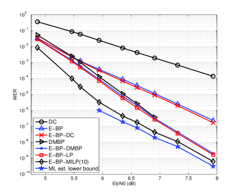
(a) Results when $T_{\max}=50$ iterations

(b) Results when $T_{\max}=300$ iterations

Figure 3: Error performance comparisons for a length-1057, rate-0.77 random LDPC code over the BSC.

From Figure 3, we also observe that the pure DC decoder needs many more iterations to obtain good performance compared with both BP and DMBP. For 300 iterations, DC performs better than E-BP at lower SNR, but exhibits an apparent error floor as the SNR increases. This high error floor is mostly the result of the DC decoder returning a codeword with lower probability than the transmitted codeword. For example, for an SNR of 6.60 dB, 80% of DC errors are of this type, while for an SNR of 7.31 dB, the percentage rises to 98%. In contrast, the BP and DMBP decoders essentially never make this kind of error.

Notice that E-BP-LP has a very similar performance to DMBP, and also that E-BP-MILP with 10 fixed bits performs the best among all the decoders and almost approaches the estimated ML lower bound. However, DMBP decoders should be significantly more practical to construct in hardware, because they are message-passing decoders similar to existing BP decoders, while LP and MILP decoders do not currently have efficient and hardware-friendly message-passing implementations.

Figure 4 depicts the WER performance comparison of the length-2209 array LDPC code over the BSC. For this QC-LDPC code, we observe broadly similar performance to the random LDPC code.

(a) Results when $T_{\max}=50$ iterations

(b) Results when $T_{\max}=300$ iterations

Figure 4: Error performance comparisons for a length-2209, rate-0.916 array LDPC code over the BSC.

Figure 5 shows the WER performance comparison of the length-1057 random LDPC code over the AWGN channel. We observe that the BP decoder for this code exhibits an error floor. DMBP improves the error floor performance compared with BP and does not have an apparent error floor. When 200 iterations are used, the DC decoder has a similar performance to BP. In the high SNR region, the DC decoder does not converge to an incorrect codeword as frequently as it does over the BSC. Note also that on the AWGN channel, while the DMBP decoder outperforms BP in the error-floor regime, it actually starts out worse in the low SNR regime.

(a) Results when $T_{\max}=50$ iterations

(b) Results when $T_{\max}=200$ iterations

Figure 5: Error performance comparisons for a length-1057, rate-0.77 random LDPC code over the AWGN channel.

Figure 6 depicts the WER performance comparison of the length-2209 array LDPC code over the AWGN channel. For this QC-LDPC code, we observe similar performance to the random LDPC code. Note again that while all decoders benefit from additional allowed iterations, the DC decoder in particular becomes increasingly competitive as the number of allowed iterations increases.

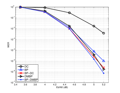
(a) Results when $T_{\max}=50$ iterations

(b) Results when $T_{\max}=200$ or $500$ iterations

Figure 6: Error performance comparisons for a length-2209 and rate-0.916 array LDPC code over the AWGN channel.

Our basic motivation for the DC and DMBP decoders was that the difference-map dynamics may help a decoder avoid dynamical “traps” that could be related to the trapping sets that are believed to cause error floors. The very good performance of the DMBP decoder in the error floor regime indicates that there may in fact be a reduction in the number of trapping sets, but on the other hand, some trapping sets clearly continue to exist, even for the DMBP decoder. In particular, we followed the approach of [6] and performed some preliminary investigations of individual “absorbing sets” in the array code that they studied, and found that although the DMBP decoder performed better on average than the BP decoder, it still would not escape if started sufficiently close to particular difficult absorbing sets.

VI Conclusion

In this paper, we investigate two decoders for LDPC codes: a DC decoder that directly applies the divide and concur approach to decoding LDPC codes, and a DMBP decoder that imports the difference-map idea into a min-sum BP-type decoder. The DMBP decoder shows particularly promising improvements in error-floor performance compared with the standard sum-product BP decoder, with comparable computational complexity, and is amenable to hardware implementation.

The DMBP decoder can be criticized for lacking a solid theoretical basis: it was constructed using intuitive ideas and is mostly interesting because of its excellent performance. The fact that its performance closely parallels that of linear programming decoders suggests that it might be related to them. In fact, our work was partially motivated by our earlier results which showed that LP decoders can significantly improve upon BP performance in the error floor regime [17]; we aimed to develop a message-passing decoder that could reproduce LP performance with complexity similar to BP.

Work in the direction of creating an efficient message-passing linear programming decoder that could replace LP solvers that relied on simplex or interior point methods was begun by Vontobel and Koetter [30], and message-passing algorithms that converge to an LP solution for some problems were suggested by Globerson and Jaakkola [31]. Our DMBP update equations are quite similar to those in the GEMPLP algorithm suggested by Globerson and Jaakkola, but our limited experiments with a GEMPLP decoder show that it does not reproduce LP decoding performance. For that matter, we have been unable to devise any other message-passing decoder with complexity similar to BP that exactly reproduces linear programming decoding. Elucidating the precise relationship between DMBP and LP decoders remains an outstanding theoretical problem, but from the practical point of view, our results show that the DMBP decoder already serves as an efficient message-passing decoder that significantly improves error floor performance compared with standard BP.

References

- [1] T. Richardson and R. Urbanke, Modern Coding Theory. Cambridge University Press, 2008.
- [2] B. J. Frey, R. Koetter, and A. Vardy, “Signal-space characterization of iterative decoding”, IEEE Trans. Inform. Theory, vol. 47, Feb. 2001, pp. 766-781.
- [3] P. O. Vontobel and R. Koetter, “Graph-cover decoding and finite-length analysis of message-passing iterative decoding of LDPC codes,” to appear in IEEE Trans. Inform. Theory http://www.arxiv.org/abs/cs.IT/0512078.
- [4] D. MacKay and M. Postol, “Weaknesses of Margulis and Ramanujan-Margulis low-density parity-check codes,” Electronic Notes in Theoretical Computer Science, vol. 74, 2003.
- [5] T. Richardson, “Error floors of LDPC codes,” Proc. 41st Allerton Conf. on Communications, Control, and Computing, Allerton House, Monticello, IL, Oct. 2003.
- [6] L. Dolecek, P. Lee, Z. Zhang, V. Anatharam, B. Nikolic, and M.J. Wainwright, “Predicting error floors of structured LDPC codes: deterministic bounds and estimates,” to appear in IEEE Jour. Sel. Areas in Comm., 2009.
- [7] See www.hpl.hp.com/personal/Pascal_Vontobel/pseudocodewords/papers/ for a collection of papers on pseudocodewords and related ideas.
- [8] X.-Y. Hu, E. Eleftheriou, and D. M. Arnold. “Regular and irregular progressive edge-growth Tanner graphs,” IEEE Trans. Inform. Theory, vol. 51, no. 1, Jan. 2005, pp. 386–398.
- [9] T. Tian, C. Jones, J. D. Villasenor, and R. D. Wesel, “Construction of irregular LDPC codes with low error floors,” IEEE International Conference on Communications, vol. 5, Anchorage, AK, May 2003, pp. 3125–3129.
- [10] Y. Wang, J. S. Yedidia, S. C. Draper, “Construction of high-girth QC-LDPC codes,” Fifth International Symposium on Turbo Codes and Related Topics 2008. Available online at http://www.merl.com/publications/TR2008-061/.
- [11] J. Zhang, J. S. Yedidia, M. P. C. Fossorier, “Low-latency decoding of EG LDPC codes,” Journal of Lightwave Technology, vol. 25, Sept. 2007, pp. 2879–2886.
- [12] R. M. Tanner, “A recursive approach to low complexity codes,” IEEE Trans. Inform. Theory, vol. 27, Sept. 1981, pp. 533–547.
- [13] Y. Wang and M. Fossorier, “Doubly generalized LDPC codes,” IEEE Int. Symp. on Inform. Theory, Seattle, WA, Jul. 2006. pp. 669–673.
- [14] R. G. Gallager, Low-Density Parity-Check Codes. Cambridge, MA: M.I.T. Press, 1963.
- [15] Y. Han and W. E. Ryan, “Low-floor decoders for LDPC codes,” Forty-Fifth Annual Allerton Conference, Allerton, IL, Sept. 2007, pp. 473–479.
- [16] S. C. Draper, J. S. Yedidia, and Y. Wang, “ML decoding via mixed-integer adaptive linear programming,” Proc. IEEE Int. Symp. Information Theory, Nice, France, Jun. 2007, pp. 1656–1660.
- [17] Y. Wang, J. S. Yedidia, and S. C. Draper , “Multi-stage decoding of LDPC codes,” Proc. IEEE Int. Symp. Information Theory, Seoul, Korea, Jun. 2009. pp. 2151–2155.
- [18] S. Gravel and V. Elser, “Divide and concur: a general approach to constraint satisfaction,” Phys. Rev. E 78, 2008. p. 036706. Available online at arXiv:0801.0222v1.
- [19] M. Mézard and A. Montanari, Information, Physics, and Computation, Oxford University Press, 2009. Chapter 8.
- [20] S. Gravel, Using Symmetries to Solve Asymmetric Problems, Ph.D. Thesis, Cornell University 2009. See section 5.4.
- [21] J. R. Fienup, “Phase retrieval algorithms: a comparison,” Applied Optics, vol. 21, 1982, pp. 2758–2769.
- [22] V. Elser, I. Rankenburg, and P. Thibault, “Searching with iterated maps,” Proc. Nat. Acad. Sci. USA, vol. 104, 2007, pp. 418–423.
- [23] H. H. Baushke, P. L. Combettes, and D. R. Luke, “Phase retrieval, error reduction algorithm, and Fienup variants: a view from convex optimization,” J. Op. Soc. Am. A, vol. 19, July 2002, pp. 1334-1345.
- [24] F. R. Kschischang, B. J. Frey, and H.-A. Loeliger, “Factor graphs and the sum-product algorithm,” IEEE Trans. on Info. Theory, vol. 47, Feb. 2001, pp. 498–519.
- [25] “Encyclopedia of Sparse Graph Codes,”, available online at http://www.inference.phy.cam.ac.uk/mackay/codes/data.html. Code 1057.244.3.457.
- [26] J. L. Fan, “Array codes as low-density parity-check codes,” Proc. 2nd Int. Symp. Turbo Codes, Brest, France, Sept. 2000, pp. 545–546.
- [27] T. J. Richardson and R. Urbanke, “The capacity of low-density parity-check codes under message-passing decoding,” IEEE Trans. on Info. Theory, vol. 47, Feb. 2001, pp. 599–618.
- [28] M.-H. N. Taghavi and P. H. Siegel, “Adaptive methods for linear programming decoding,” IEEE Trans. Inform. Theory, vol. 54, Dec. 2008, pp. 5396-5410.
- [29] “GNU Linear Programming Kit,” http://www.gnu.org/software/glpk.
- [30] P. Vontobel and R. Koetter, “Towards low-complexity linear-programming decoding,” Proc. 4th Int. Symposium on Turbo Codes and Related Topics, Munich, Germany, 2006.
- [31] A. Globerson and T. Jaakkola, “Fixing max-product: convergent message passing algorithms for MAP LP-relaxations,” Advances in Neural Information Processing Systems 20, Vancouver, Canada, 2007.