Statistical Isotropy violation of the CMB brightness fluctuations

Abstract

Certain anomalies at large angular scales in the cosmic microwave background measured by WMAP have been suggested as possible evidence of breakdown of statistical isotropy(SI). SI violation of cosmological perturbations is a generic feature of ultra large scale structure of the cosmos and breakdown of global symmetries. Most CMB photons free-stream to the present from the surface of last scattering. It is thus reasonable to expect statistical isotropy violation in the CMB photon distribution observed now to have originated from SI violation in the baryon-photon fluid at last scattering, in addition to anisotropy of the primordial power spectrum studied earlier in literature.

We consider the generalized anisotropic brightness distribution fluctuations, $\Delta(\vec{k},\hat{n},\tau)$ (at conformal time $\tau$) in contrast to the SI case where it is simply a function of $|\vec{k}|$ and $\hat{k}\cdot\hat{n}$. The brightness fluctuations expanded in Bipolar Spherical Harmonic (BipoSH) series, can then be written as $\Delta_{\ell_{1}\ell_{2}}^{LM}(k,\tau)$ where $L>0$ terms encode deviations from statistical isotropy. Violation of SI encoded in the present off-diagonal elements of the harmonic space correlation $\langle a_{\ell m}a_{\ell^{\prime}m^{\prime}}^{*}\rangle$, equivalently, the BipoSH coefficients $A^{LM}_{\ell\ell^{\prime}}$, are then related to the generalized BipoSH brightness fluctuation terms at present. We study the evolution of $\Delta_{\ell_{1}\ell_{2}}^{LM}(k,\tau)$ from non-zero terms $\Delta_{\ell_{3}\ell_{4}}^{LM}(k,\tau_{s})$ at last scattering, in the free streaming regime. We show that the terms with given BipoSH multipole, $LM$, evolve independently. Moreover, similar to the SI case, power at small spherical harmonic (SH) multipoles of $\Delta_{\ell_{3}\ell_{4}}^{LM}(k,\tau_{s})$ at the last scattering, is transferred to $\Delta_{\ell_{1}\ell_{2}}^{LM}(k,\tau)$ at larger SH multipoles. The structural similarity is more apparent in the asymptotic expression for large values of the final SH multipoles. This formalism allows an elegant identification of any SI violation observed today to a possible origin in SI violating physics present in the baryon-photon fluid. This is illustrated for the known result of SI violating angular correlations due to the presence of a homogeneous magnetic field in the baryon-photon fluid.

I Introduction

The Cosmic Microwave Background (CMB) anisotropy is a very powerful observational probe of cosmology. In standard cosmology, CMB anisotropy signal is expected to be statistically isotropic, i.e., statistical expectation values of the temperature fluctuations $\Delta T(\hat{n})=\sum_{\ell m}a_{\ell m}Y_{\ell m}(\hat{n})$ are preserved under rotations of the sky. The condition for statistical isotropy (SI), in spherical harmonic space translates to a diagonal $\langle a_{\ell m}a_{\ell^{\prime}m^{\prime}}^{*}\rangle=C_{\ell}\delta_{\ell\ell^{\prime}}\delta_{mm^{\prime}}$ where $C_{\ell}$ is the widely used angular power spectrum of the CMB anisotropy.

After the release of first year data of the Wilkinson Microwave Anisotropy Probe (WMAP), statistical isotropy of the CMB anisotropy attracted considerable attention. The study of full sky maps from the WMAP 5 year data Komatsu et al. (2009); Spergel et al. (2007); Nolta et al. (2009) and the very recent WMAP 7 year data Bennett et al. (2010), has led to some intriguing anomalies which seem to suggest that the assumption of statistical isotropy is broken on the largest angular scales de Oliveira-Costa et al. (2004); Copi et al. (2007); Hansen et al. (2009); Eriksen et al. (2007); Hoftuft et al. (2009). Broken isotropy would have a profound implications for standard cosmological model as statistical isotropy underlies all cosmological inferences.

It was pointed out that the suppression of power in the quadrupole and octopole are aligned in the form of the “ axis of evil” Land and Magueijo (2005); Tegmark et al. (2003); Magueijo and Sorkin (2007); Rakic and Schwarz (2007); Frommert and Ensslin (2010). Further “multipole-vector” directions associated with these multipoles (and some other low multipoles as well) appear to be anomalously correlated Copi et al. (2007), Copi et al. (2004), Schwarz et al. (2004). There are indications of asymmetry in the power spectrum at low multipoles in opposite hemispheres, the “north-south asymmetry” Hansen et al. (2009), Eriksen et al. (2007), Eriksen et al. (2004a); Hansen et al. (2004); Naselsky et al. (2005). Possibly related, are the results of tests of Gaussianity that show asymmetry in the amplitude of the measured genus amplitude (at about 2 to 3 $\sigma$ significance) between the north and south galactic hemispheres Park (2004); Eriksen et al. (2004b, c). Analysis of the distribution of extrema in WMAP sky maps has indicated non-Gaussianity, and to some extent, violation of SI Larson and Wandelt (2004).

An observed map of CMB anisotropy, $\Delta T(\hat{n})^{\mathrm{obs}}$ contains the true CMB temperature $\Delta T(\hat{n})$ fluctuations, convolved with the beam and instrumental noise & foreground contaminations. Breakdown of statistical isotropy can occur in any of these parts and can be categorized as

• Theoretically motivated effects which are intrinsic to the true CMB sky, $\Delta T(\hat{n})$ include non-trivial cosmic topology Souradeep (2006), Bianchi models Jaffe et al. (2005, 2006); Pontzen and Challinor (2007); Ghosh et al. (2007) and primordial magnetic fields Durrer et al. (1998), Kahniashvili et al. (2008). A recent article Urban and Zhitnitsky (2009) claims that the solution to the cosmological vacuum energy can be explained as a result of the interaction of the infrared sector of the effective theory of gravity with standard model fields. This theory predicts the violation of cosmological isotropy.

• Although a possible source of SI breakdown, residual foreground contamination would need to be of order the intrinsic CMB temperature anisotropy to account for an appreciable effect Copi et al. (2006); Hinshaw et al. (2009); Gold et al. (2009).

• It would be erroneous to assume that the true CMB temperature fluctuations are completely extracted from the observed map. Observational artifacts such as non-circular beam, inhomogeneous noise correlation, residual striping patterns could be potential sources of SI breakdown.

Violation of statistical isotropy of CMB anisotropy and its measurement has been discussed in literature earlier Hajian and Souradeep (2003a); Hajian and Souradeep (2003b); Souradeep and Hajian (2004); Hajian and Souradeep (2004, 2006); Souradeep et al. (2006) by defining an estimator where SI breakdown in an observed CMB anisotropy sky map is indicated by non zero value of this estimator. Studies have also been done by implementing a directional dependent inflationary power spectrum $P(\vec{k})$ which gives rise to off-diagonal terms in the covariance matrix Ackerman et al. (2007), Pullen and Kamionkowski (2007); spontaneous breakdown of SI in the CMB by a non-linear response to long-wavelength field fluctuations that appear as a gradient locally to the observer Gordon et al. (2005) or locally through a modulation field Dvorkin et al. (2008); incorporating an initial period of kinetic energy domination in single field inflation Donoghue et al. (2009).

In this paper we present a new formulation that relates the breakdown of SI in the CMB photon fluctuations at last scattering, and evolving them to find the effect of the modes at present epoch hence the CMB $\langle a_{\ell m}a_{\ell^{\prime}m^{\prime}}\rangle$ today. We also find the Bipolar spherical harmonic coefficients (BipoSH) Hajian and Souradeep (2004, 2006) which are linear combinations of off-diagonal elements of the covariance matrix. BipoSH expansion completely represents the information of the covariance matrix thus being the most general way of studying two point correlation functions of CMB anisotropy. These BipoSH coefficients are mathematically complete measures of SI violation on a sphere.

II Review of Statistically Isotropic CMB brightness fluctuations

II.1 Boltzmann equations, inhomogeneities and anisotropies

In the smooth background universe, thermalized photons being distributed homogeneously and isotropically, the temperature $T$ is independent of $\vec{x}$ and direction of propagation $\hat{p}$ respectively. To describe perturbations about this smooth universe, we allow inhomogeneities in the photon distribution and anisotropies.

Before recombination, $z_{\mathrm{rec}}\approx 1100$, the photons were tightly coupled to the electrons and protons; all together they can be described as a single fluid, the baryon-photon fluid. After recombination, photons free-stream from the surface of last scattering to the present epoch.

Given the cosmological perturbations to the photons at recombination, one can predict the anisotropy spectrum today. The main motivation next is to relate the moments today to the moments at recombination using the photon distribution function.

II.2 Fluctuations of CMB photon distribution

In the Boltzmann equation for photons $df/dt=C[f]$, we expand the photon distribution function $f(\vec{x},p,\hat{n},\tau)$ about its zero-order Bose-Einstein value $T(\tau)$ Dodelson (2003) where $\vec{p}=p\hat{n}$. The distribution function of the photons changes with the perturbed temperature as

$$f(\vec{x},p,\hat{n},\tau)=\left[\mathrm{exp}\left\{\frac{p}{T(\tau)[1+\Delta(\vec{x},\hat{n},\tau)]}\right\}-1\right]^{-1}.$$ (1)

The perturbation to the distribution function is characterized by $\Delta\equiv\delta T/T$ termed as CMB brightness fluctuations henceforth. Since the perturbation $\Delta$ is small, we can expand $f(\vec{x},p,\hat{n},\tau)$ keeping only terms up to first order to get

$$\Delta(\vec{x},\hat{n},\tau)\equiv\left(\frac{\partial f^{0}}{\partial\ln p}\right)^{-1}\delta f,$$ (2)

where $f^{0}$ is the zero-order photon distribution function. $\Delta(\vec{x},\hat{n},\tau)$ depends on $\vec{x},\hat{n}$ and $\tau$ and not on the magnitude of momentum $p$; this is a valid assumption since the temperature of the plasma is very small compared to the rest energy of the electrons which undergo scattering, elastic Thomson scattering has negligible effect on the magnitude of the photon momentum.

Perturbations to the CMB remain small at all cosmological epochs; evolution of the largest scales being in the linear regime. In solving the linear evolution equations, it is simplest to work with Fourier transforms since every Fourier mode evolves independently.

$$\Delta(\vec{x},\hat{n},\tau)=\int\frac{d^{3}k}{(2\pi)^{3}}e^{i\vec{k}\cdot\vec{x}}\tilde{\Delta}(\vec{k},\hat{n},\tau)\phi(\vec{k})\;,$$ (3)

where $\phi(\vec{k})$ is the primordial density fluctuations.

With statistical isotropy assumption

$$\tilde{\Delta}(\vec{k},\hat{n},\tau) = \tilde{\Delta}(k,\hat{k}\cdot\hat{n},\tau)$$ (4)

$$= \sum_{\ell}(-i)^{\ell}(2\ell+1)\tilde{\Delta}_{\ell}(k,\tau)P_{\ell}(\hat{k}\cdot\hat{n})$$

$$= 4\pi\sum_{\ell m}(-i)^{\ell}\tilde{\Delta}_{\ell}(k,\tau)Y_{\ell m}(\hat{k})Y_{\ell m}(\hat{n}).$$

$\tilde{\Delta}_{\ell}(k,\tau)$ are the moments of the CMB brightness fluctuation. The monopole $\tilde{\Delta}_{0}$ is related to the density perturbations while the dipole $\tilde{\Delta}_{1}\propto\hat{n}\cdot\vec{v}$, gives the velocity term for baryons.

II.3 Correlations

The observed anisotropy in multipole space can be written in terms of the CMB brightness fluctuation as

$$\Delta(\vec{x}=0,\hat{n},\tau)=\sum_{\ell m}a_{\ell m}Y_{\ell m}(\hat{n})\;.$$ (5)

Using the orthonormality property of the spherical harmonics $Y_{\ell m}$, the SH coefficients $a_{\ell m}$ become

$$a_{\ell m}=4\pi(-i)^{\ell}\int\frac{d^{3}k}{(2\pi)^{3}}\;\phi(\vec{k})\tilde{\Delta}_{\ell}(k,\tau)Y_{\ell m}^{*}(\hat{k}).$$ (6)

The angular correlation can be expressed as

$$\langle a_{\ell m}a_{\ell^{\prime}m^{\prime}}^{*}\rangle = 4\pi\int\frac{dk}{k}\frac{k^{3}P_{0}(k)}{2\pi^{2}}|\Delta_{\ell}(k,\tau)|^{2}\delta_{\ell\ell^{\prime}}\delta_{mm^{\prime}}$$

$$C_{\ell} = 4\pi\int\frac{dk}{k}\mathcal{P}_{0}(k)|\Delta_{\ell}(k,\tau)|^{2}\;,$$ (7)

where correlation of the primordial density fluctuations $\langle\phi(\vec{k})\phi^{*}(\vec{k^{\prime}})\rangle=P_{0}(k)\delta(\vec{k}-\vec{k^{\prime}})$ and $\mathcal{P}_{0}(k)=k^{3}P_{0}(k)/2\pi^{2}$ is the primordial power spectrum per logarithmic interval generated by inflationary model and the second term is the radiative transport kernel in the post-recombination universe given by cosmological parameters.

II.4 Evolution of CMB brightness fluctuation in the free-streaming regime

The evolution of ​ $\tilde{\Delta}(\vec{k},\hat{n},\tau)$ in the free-streaming regime can be written as

$$\tilde{\Delta}(\vec{k},\hat{n},\tau)=e^{i\vec{k}\cdot\hat{n}(\tau-\tau_{s})}\tilde{\Delta}(\vec{k},\hat{n},\tau_{s}),$$ (8)

where $\tau$ is well inside the free-streaming regime i.e. $\tau_{s}<\tau<\tau_{0}$, $\tau_{s}$ and $\tau_{0}$ being the conformal time at last scattering and today respectively Bond and Efstathiou (1984).

Using the expansion

$$e^{i\vec{k}\cdot\hat{n}\Delta\tau}=\sum_{l}(-i)^{l}(2l+1)j_{l}(k\Delta\tau)P_{l}(\hat{k}\cdot\hat{n}),$$ (9)

and defining $\Delta\tau=\tau-\tau_{s}$, the evolution equation for $\tilde{\Delta}_{\ell}(k,\tau)$ can be written as

$$\tilde{\Delta}_{\ell}(k,\tau) = \sum_{l\ell^{\prime}}(-i)^{\ell+\ell^{\prime}-l}\>(2\ell^{\prime}+1)\>j_{l}(k\Delta\tau)$$ (10)

$$\times [\mathcal{C}^{l0}_{\ell 0\ell^{\prime}0}]^{2}\>\tilde{\Delta}_{\ell^{\prime}}(k,\tau_{s}).$$

$j_{l}(k\Delta\tau)$ and $P_{l}(\hat{k}\cdot\hat{n})$ are the $\ell^{\mathrm{th}}$ order spherical Bessel function and Legendre Polynomial, respectively. Equation (10) is the well known “free streaming ” equation in CMB literature Bond and Efstathiou (1984). $\mathcal{C}^{LM}_{\ell_{1}m_{1}\ell_{2}m_{2}}$ are the Clebsch-Gordan coefficient which satisfies the triangle inequalities (Varshalovich et al. (1988)) putting a constraint $|\ell_{1}-\ell_{2}|\leq L\leq\ell_{1}+\ell_{2}$ and $m_{1}+m_{2}=M$.

III Statistical isotropy breakdown in the CMB brightness fluctuation

In this paper we take into account the SI violation of the CMB anisotropy which is seeded due to the inherent SI breakdown in the CMB photon distribution. We consider the general form of the CMB brightness fluctuation, allowing for anisotropy in $\hat{k}$, i.e., $\tilde{\Delta}(\vec{k},\hat{n},\tau)\not\equiv\tilde{\Delta}(k,\hat{k}\cdot\hat{n},\tau)$.

III.1 Generalized CMB brightness fluctuations

The most general CMB brightness fluctuation is not simply a function of $|\vec{k}|$ and $\hat{k}\cdot\hat{n}$. In this case the physical situation of anisotropic fluctuations demand the brightness fluctuations to be expanded in Bipolar Spherical Harmonic series (not just a Legendre series as in the statistical isotropic case). The brightness fluctuation in multipole space is $\Delta_{\ell_{1}\ell_{2}}^{LM}(\vec{k},\tau)$ where $L>0$ term incorporates deviation from statistical isotropy.

$$\tilde{\Delta}(\vec{k},\hat{n},\tau) = 4\pi\sum_{\ell_{1}\ell_{2}LM}(i)^{\frac{\ell_{1}+\ell_{2}}{2}}\sqrt{\ell_{1}+\ell_{2}+1}$$ (11)

$$\times \tilde{\Delta}_{\ell_{1}\ell_{2}}^{LM}(k,\tau)\;\{Y_{\ell_{1}}(\hat{k})\otimes Y_{\ell_{2}}(\hat{n})\}_{LM}$$

$$= 4\pi\sum_{\ell_{1}\ell_{2}LM}\beta_{\ell_{1}\ell_{2}}\;\tilde{\Delta}_{\ell_{1}\ell_{2}}^{LM}(k,\tau)$$

$$\times \{Y_{\ell_{1}}(\hat{k})\otimes Y_{\ell_{2}}(\hat{n})\}_{LM},$$

where $\beta_{\ell_{1}\ell_{2}}=(i)^{\frac{\ell_{1}+\ell_{2}}{2}}\sqrt{\ell_{1}+\ell_{2}+1}$ has been defined for convenient notational simplicity.

The tensor product in BipoSH function is defined as

$$\{Y_{\ell_{1}}(\hat{k})\!\otimes\!Y_{\ell_{2}}(\hat{n})\}_{LM} = \sum_{m_{1}m_{2}}\mathcal{C}^{LM}_{\ell_{1}m_{1}\ell_{2}m_{2}}$$

$$\times Y_{\ell_{1}m_{1}}(\hat{k})\;Y_{\ell_{2}m_{2}}(\hat{n}).$$

The pre-factors in equation (11) are the normalization terms associated with the CMB brightness fluctuation. The deviations from statistical isotropy is associated with non-zero values of $L,\;L>0$. To check for the statistical isotropy limit i.e. $L=0$ & $M=0$, we use equation (8.5.1) from Varshalovich et al. (1988)

$$\mathcal{C}^{00}_{\ell_{1}m_{1}\ell_{2}m_{2}}=(-1)^{\ell_{1}-m_{1}}\frac{\delta_{\ell_{1}\ell_{2}}\delta_{m_{1}\,-m_{2}}}{\sqrt{2\ell_{1}+1}},$$ (12)

to recover equation (4) in section (II.2).

III.2 Angular Correlations

Starting with equation (5) and the Fourier Transform relation from equation (3), the SH coefficients $a_{\ell m}$ for the general case are

$$a_{\ell m} = 4\pi\int\frac{d^{3}k}{(2\pi)^{3}}\;\phi(\vec{k})\sum_{\ell_{1}m_{1}LM}\beta_{\ell_{1}\ell}\;\tilde{\Delta}_{\ell_{1}\ell}^{LM}(k,\tau)$$ (13)

$$\times \mathcal{C}^{LM}_{\ell_{1}m_{1}\ell m}\;Y_{\ell_{1}m_{1}}(\hat{k}).$$

The angular correlations turn out to be

$$\langle a_{\ell m}a_{\ell^{\prime}m^{\prime}}^{*}\rangle = (4\pi)^{2}\int\int\frac{d^{3}k}{(2\pi)^{3}}\frac{d^{3}k^{\prime}}{(2\pi)^{3}}\langle\phi(\vec{k})\phi^{*}(\vec{k^{\prime}})\rangle$$ (14)

$$\times \sum_{\ell_{1}m_{1}LM}\sum_{\ell_{2}m_{2}L^{\prime}M^{\prime}}\beta_{\ell_{1}\ell}\beta_{\ell_{2}\ell^{\prime}}^{*}$$

$$\times \mathcal{C}^{LM}_{\ell_{1}m_{1}\ell m}\mathcal{C}^{L^{\prime}M^{\prime}}_{\ell_{2}m_{2}\ell^{\prime}m^{\prime}}\;Y_{\ell_{1}m_{1}}(\hat{k})Y^{*}_{\ell_{2}m_{2}}(\hat{k^{\prime}})$$

$$\times \tilde{\Delta}_{\ell_{1}\ell}^{LM}(k,\tau)[\tilde{\Delta}_{\ell_{2}\ell^{\prime}}^{L^{\prime}M^{\prime}}(k^{\prime},\tau)]^{*}.$$

The most general power spectrum (under statistical homogeneity) depends on the direction $\hat{k}$,

$$\langle\phi(\vec{k})\phi^{*}(\vec{k^{\prime}})\rangle=P(\vec{k})\delta(\vec{k}-\vec{k^{\prime}}).$$ (15)

Further, it is useful to parametrize the directional dependence of $\hat{k}$ in $P(\vec{k})$ as Pullen and Kamionkowski (2007)

$$P(\vec{k})=P_{0}(k)\left[1+\sum_{\mathfrak{l}>0}\sum_{\mathfrak{m}=-\mathfrak{l}}^{\mathfrak{l}}g_{\mathfrak{l}\mathfrak{m}}(k)\;Y_{\mathfrak{l}\mathfrak{m}}(\hat{k})\right],$$ (16)

where the first term with $\mathfrak{l}=0$ represents the statistical homogeneous and isotropic primordial power spectrum.

For a directional dependent power spectrum, the angular correlations of temperature anisotropy can be written as

$$\langle a_{\ell m}a_{\ell^{\prime}m^{\prime}}^{*}\rangle = 4\pi\!\!\int\frac{k^{2}dk}{2\pi^{2}}P_{0}(k)\!\!\!\!\!\!\sum_{\ell_{1}m_{1}LML^{\prime}M^{\prime}}\left[D_{1}\tilde{\Delta}_{\ell_{1}\ell}^{LM}(k,\tau)\right.$$ (17)

$$\times [\tilde{\Delta}_{\ell_{1}\ell^{\prime}}^{L^{\prime}M^{\prime}}(k,\tau)]^{*}+\sum_{\ell_{2}m_{2}\mathfrak{l}\mathfrak{m}}D_{2}\;g_{\mathfrak{l}\mathfrak{m}}(k)$$

$$\times \left.\tilde{\Delta}_{\ell_{1}\ell}^{LM}(k,\tau)\;[\tilde{\Delta}_{\ell_{2}\ell^{\prime}}^{L^{\prime}M^{\prime}}(k,\tau)]^{*}\;\mathcal{Y}^{\ell_{2}m_{2}}_{\ell_{1}m_{1},\mathfrak{l}\mathfrak{m}}\right],$$

where

$$D_{1} = \beta_{\ell_{1}\ell}\;\beta^{*}_{\ell_{1}\ell^{\prime}}\;\mathcal{C}^{LM}_{\ell_{1}m_{1}\ell m}\;\mathcal{C}^{L^{\prime}M^{\prime}}_{\ell_{1}m_{1}\ell^{\prime}m^{\prime}},$$

$$D_{2} = \beta_{\ell_{1}\ell}\;\beta^{*}_{\ell_{2}\ell^{\prime}}\;\mathcal{C}^{LM}_{\ell_{1}m_{1}\ell m}\;\mathcal{C}^{L^{\prime}M^{\prime}}_{\ell_{2}m_{2}\ell^{\prime}m^{\prime}},$$

$$\mathcal{Y}^{\ell_{2}m_{2}}_{\ell_{1}m_{1},\mathfrak{l}\mathfrak{m}} = \int d\Omega_{\hat{k}}\;Y_{\ell_{1}m_{1}}(k)\;Y^{*}_{\ell_{2}m_{2}}(k)\;Y_{\mathfrak{l}\mathfrak{m}}(k)$$

$$= \frac{\Pi_{\ell_{1}\mathfrak{l}}}{\sqrt{4\pi}\;\Pi_{\ell_{2}}}\mathcal{C}^{\ell_{2}0}_{\ell_{1}0\mathfrak{l}0}\mathcal{C}^{\ell_{2}m_{2}}_{\ell_{1}m_{1}\mathfrak{l}\mathfrak{m}},$$

where we have used the expression for integral of three spherical harmonics as in equation (5.9.4) from Varshalovich et al. (1988).

Here $\Pi_{\ell_{1}\ell_{2}...\ell_{n}}=[(2\ell_{1}+1)(2\ell_{2}+1)...(2\ell_{n}+1)]^{\frac{1}{2}}$ has been defined for convenient notational simplicity.

The case $L=0$ reduces equation (17) to that in the analysis Pullen and Kamionkowski (2007)

$$\langle a_{\ell m}a_{\ell^{\prime}m^{\prime}}^{*}\rangle = \frac{(-1)^{\ell}}{\Pi_{\ell}}A^{00}_{\ell\ell^{\prime}}\delta_{\ell\ell^{\prime}}\delta_{mm^{\prime}}$$ (18)

$$+ (-1)^{\ell^{\prime}+m^{\prime}}\sum_{\mathfrak{l},\mathfrak{m}}A^{\mathfrak{l}\mathfrak{m}}_{\ell\ell^{\prime}}\;\;\mathcal{C}^{\mathfrak{l}\mathfrak{-m}}_{\ell m\ell^{\prime}m^{\prime}},$$

where statistical anisotropy is quantified by the BipoSH coefficients Hajian and Souradeep (2003b, 2004, 2006); Souradeep et al. (2006), defined as a tensor product of the spherical harmonic coefficients $a_{\ell m}$ and $a_{\ell^{\prime}m^{\prime}}$,

$$A^{JN}_{\ell\ell^{\prime}} = \sum_{mm^{\prime}}\langle a_{\ell m}a_{\ell^{\prime}m^{\prime}}^{*}\rangle(-1)^{m^{\prime}}\mathcal{C}^{JN}_{\ell m\ell^{\prime}-m^{\prime}}$$

$$= \left\{a_{\ell}\otimes a_{\ell^{\prime}}\right\}_{JN}\;$$

$$A_{\ell\ell}^{00} = (-1)^{\ell}\;\Pi_{\ell}\;C_{\ell}$$ (19)

Here, $C_{\ell}$ is the usual CMB power spectrum for the SI case. Directional dependent $P(\hat{k})$ Pullen and Kamionkowski (2007), introduces the second term in equation (18)

$$A^{\mathfrak{l}\mathfrak{m}}_{\ell\ell^{\prime}} = \sqrt{4\pi}(-i)^{\ell+\ell^{\prime}}\frac{\Pi_{\ell}\Pi_{\ell^{\prime}}}{\Pi_{\mathfrak{l}}}\int\frac{k^{2}dk}{2\pi^{2}}\;P_{0}(k)g_{\mathfrak{l}\mathfrak{m}}$$ (20)

$$\times \mathcal{C}^{\mathfrak{l}0}_{\ell 0\ell^{\prime}0}\left\{\tilde{\Delta}^{0}_{\ell\ell}\otimes\tilde{\Delta}^{0}_{\ell^{\prime}\ell^{\prime}}\right\}_{00},$$

where a corresponding tensor product in Bipolar harmonic space for the indices $L$ and $L^{\prime}$ of CMB brightness fluctuations is defined as

$$\left\{\tilde{\Delta}^{L}_{\ell_{1}\ell}\otimes\tilde{\Delta}^{L^{\prime}}_{\ell_{2}\ell^{\prime}}\right\}_{JN} = \sum_{MM^{\prime}}(-1)^{M^{\prime}}\mathcal{C}^{JN}_{LML^{\prime}-M^{\prime}}$$ (21)

$$\times \tilde{\Delta}_{\ell_{1}\ell}^{LM}(k,\tau)[\tilde{\Delta}_{\ell_{2}\ell^{\prime}}^{L^{\prime}M^{\prime}}(k,\tau)]^{*}\!.$$

In general for SI violations $(L>0)$, the BipoSH coefficients can be expressed using the angular correlations in equation (17) as shown in Appendix A as

$$A^{JN}_{\ell\ell^{\prime}} = \left(A^{JN}_{\ell\ell^{\prime}}\right)_{\mathfrak{l}=0}+\sqrt{4\pi}\int\frac{k^{2}dk}{2\pi^{2}}P_{0}(k)$$ (25)

$$\times \sum_{\mathfrak{l}\ell_{1}\ell_{2}LL^{\prime}}\!\!\!\Pi_{\mathfrak{l}\ell_{1}LL^{\prime}}(-1)^{\mathfrak{l}+L^{\prime}+\ell^{\prime}+\ell_{1}-\ell_{2}}\beta_{\ell_{1}\ell}\beta_{\ell_{2}\ell^{\prime}}^{*}$$

$$\times \mathcal{C}^{\ell_{2}0}_{\ell_{1}0\mathfrak{l}0}\sum_{\mathfrak{m}}g_{\mathfrak{l}\mathfrak{m}}\sum_{\ell_{3}m_{3}}\left\{\begin{array}[]{ccc}\!J\!&\ell_{3}\!&\mathfrak{l}\!\\ \!\ell\!&L\!&\ell_{1}\!\\ \!\ell^{\prime}\!&L^{\prime}\!&\ell_{2}\!\end{array}\right\}$$

$$\times \mathcal{C}^{JN}_{\ell_{3}m_{3}\mathfrak{l}\mathfrak{m}}\left\{\tilde{\Delta}^{L}_{\ell_{1}\ell}\otimes\tilde{\Delta}^{L^{\prime}}_{\ell_{2}\ell^{\prime}}\right\}_{\ell_{3}m_{3}}.$$ (26)

The first term on the right-hand side of equation (26), is the contribution due to statistically isotropic primordial power spectrum i.e. $\mathfrak{l}=0$ terms in equation (16). The second term gives the contribution to the Bipolar coefficients due to $\mathfrak{l}>0$ in equation (16). The term in the first braces is the Wigner-9j symbol Varshalovich et al. (1988) which is related to the coefficients of transformations between different coupling schemes of four angular momenta and satisfies the triangular conditions for the triads $(J\ell_{3}\mathfrak{l}),(\ell L\ell_{1}),(\ell^{\prime}L^{\prime}\ell_{2}),(J\ell\ell^{\prime}),(\ell_{3}LL^{\prime})$ and $(\mathfrak{l}\ell_{1}\ell_{2})$.

The SI case $L=0$ reduces the BipoSH coefficients in equation (26) to equation (20).

To evaluate the first term $\left(A^{JN}_{\ell\ell^{\prime}}\right)_{\mathfrak{l}=0}$ in equation (26), we consider statistically isotropic primordial perturbations $\langle\phi(\vec{k})\phi^{*}(\vec{k^{\prime}})\rangle=P_{0}(k)\delta(\vec{k}-\vec{k^{\prime}})$ and express the angular correlations as

$$\langle a_{\ell m}a_{\ell^{\prime}m^{\prime}}^{*}\rangle = 4\pi\int\frac{k^{2}dk}{2\pi^{2}}P_{0}(k)\sum_{\ell_{1}m_{1}LML^{\prime}M^{\prime}}\beta_{\ell_{1}\ell}\>\beta_{\ell_{1}\ell^{\prime}}^{*}\>$$ (27)

$$\times \tilde{\Delta}_{\ell_{1}\ell}^{LM}(k,\tau)\>[\tilde{\Delta}_{\ell_{1}\ell^{\prime}}^{L^{\prime}M^{\prime}}(k,\tau)]^{*}$$

$$\times \mathcal{C}^{LM}_{\ell_{1}m_{1}\ell m}\>\mathcal{C}^{L^{\prime}M^{\prime}}_{\ell_{1}m_{1}\ell^{\prime}m^{\prime}}.$$

To check for the statistical isotropic case, we put $L=0$ & $M=0$ and recover equation (7) in section (II.3).

As shown in detail in Appendix A, the BipoSH coefficients in equation (19), can be expressed using the angular correlations in equation (27) for statistically isotropic primordial perturbations as

$$(A^{JN}_{\ell\ell^{\prime}})_{\mathfrak{l}=0} = 4\pi\int\frac{k^{2}dk}{2\pi^{2}}P_{0}(k)\sum_{\ell_{1}LL^{\prime}}(-1)^{\ell_{1}+L+L^{\prime}+J}$$ (30)

$$\times \Pi_{LL^{\prime}}\>\>\beta_{\ell_{1}\ell}\>\>\beta_{\ell_{1}\ell^{\prime}}^{*}\>\left\{\begin{array}[]{ccc}L&J&L^{\prime}\\ \ell^{\prime}&\ell_{1}&\ell\end{array}\right\}$$

$$\times \left\{\tilde{\Delta}^{L}_{\ell_{1}\ell}\otimes\tilde{\Delta}^{L^{\prime}}_{\ell_{1}\ell^{\prime}}\right\}_{JN}.$$ (31)

The first term in braces is the Wigner-6j symbol which is related to the coefficients of transformations between different coupling schemes of three angular momenta. These vanish unless the triangular conditions Varshalovich et al. (1988) are fulfilled for the triads $(LJL^{\prime}),(L^{\prime}\ell^{\prime}\ell_{1}),(J\ell^{\prime}\ell)$ and $(\ell L\ell_{1})$.

We consider low Bipolar deviations from SI i.e. $L,L^{\prime}$ and $J<<\ell,\ell^{\prime},\ell_{1}$ in equation (31) and use the asymptotic relation for Wigner-6j functions given by equation (9.9.1) from Varshalovich et al. (1988). We find that the asymptotic limit to these BipoSH coefficients are

$$(A^{JN}_{\ell\ell^{\prime}})_{\mathfrak{l}=0} \approx 4\pi\int\frac{k^{2}dk}{2\pi^{2}}P_{0}(k)\sum_{\ell_{1}LL^{\prime}}(-1)^{\ell+\ell^{\prime}+\ell_{1}+L+L^{\prime}}$$ (32)

$$\times \frac{\Pi_{LL^{\prime}}}{\sqrt{2\ell_{1}}\;\Pi_{J}}\>\>\beta_{\ell_{1}\ell}\>\>\beta_{\ell_{1}\ell^{\prime}}^{*}\>\>\mathcal{C}^{J(\ell-\ell^{\prime})}_{L(\ell-\ell_{1})L^{\prime}(\ell_{1}-\ell^{\prime})}$$

$$\times \left\{\tilde{\Delta}^{L}_{\ell_{1}\ell}\otimes\tilde{\Delta}^{L^{\prime}}_{\ell_{1}\ell^{\prime}}\right\}_{JN}\;.$$

For diagonal brightness fluctuations i.e $\ell_{1}=\ell$ and $\ell_{1}=\ell^{\prime}$, the BipoSH coefficients themselves turn out to be diagonal in multipole space

$$(A^{JN}_{\ell\ell})_{\mathfrak{l}=0} \approx 4\pi\int\frac{k^{2}dk}{2\pi^{2}}P_{0}(k)\sum_{LL^{\prime}}(-1)^{L+L^{\prime}+1}\;\frac{\Pi_{\ell\ell LL^{\prime}}}{\Pi_{J}}$$ (33)

$$\times \mathcal{C}^{J0}_{L0L^{\prime}0}\left\{\tilde{\Delta}^{L}_{\ell\ell}\otimes\tilde{\Delta}^{L^{\prime}}_{\ell\ell}\right\}_{JN}.$$

IV Evolution in the free-streaming regime

IV.1 Generalized evolution equation

We find the moments of the CMB brightness fluctuation to be

$$\tilde{\Delta}_{\ell_{1}\ell_{2}}^{LM}(k,\tau) = \frac{1}{4\pi}\frac{1}{\beta_{\ell_{1}\ell_{2}}}\int\int d\Omega_{\hat{n}}\;d\Omega_{\hat{k}}\;\tilde{\Delta}(\vec{k},\hat{n},\tau)$$ (34)

$$\times \{Y_{\ell_{1}}(\hat{k})\otimes Y_{\ell_{2}}(\hat{n})\}_{LM},$$

starting with equation (11) and the orthonormality condition of BipoSH,

$$\int\!\!\!\int d\Omega_{\hat{n}}d\Omega_{\hat{k}} \!\!\!\!\!\!\!\!\!\!\!\{Y_{\ell_{1}}(\hat{k})\otimes Y_{\ell_{2}}(\hat{n})\}_{LM}\{Y_{\ell_{3}}(\hat{k})\otimes Y_{\ell_{4}}(\hat{n})\}_{L^{\prime}M^{\prime}}^{*}$$ (35)

$$= \delta_{\ell_{1}\ell_{3}}\;\delta_{\ell_{2}\ell_{4}}\>\delta_{LL^{\prime}}\delta_{MM^{\prime}}.$$

In the free streaming regime, using the plane wave approximation as in equations (8) and (9), the most general evolution equation turns out to be

$$\tilde{\Delta}_{\ell_{1}\ell_{2}}^{LM}(k,\tau) = \frac{1}{\beta_{\ell_{1}\ell_{2}}}\sum_{\ell\ell_{3}\ell_{4}L^{\prime}M^{\prime}}(-i)^{\ell}\;\Pi_{\ell\ell}\;j_{\ell}(k\Delta\tau)\;\beta_{\ell_{3}\ell_{4}}$$ (36)

$$\times \sum_{m_{1}m_{2}m_{3}m_{4}}\!\!\!\!\!\!\!\tilde{\Delta}_{\ell_{3}\ell_{4}}^{LM}(k,\tau_{s})\>\mathcal{C}^{LM}_{\ell_{1}m_{1}\ell_{2}m_{2}}\>\mathcal{C}^{L^{\prime}M^{\prime}}_{\ell_{3}m_{3}\ell_{4}m_{4}}$$

$$\times \int\!\!\!\int d\Omega_{\hat{n}}\;d{\hat{k}}\;P_{\ell}(\hat{k}\cdot\hat{n})\>Y_{\ell_{1}m_{1}}^{*}({\hat{k}})\>Y_{\ell_{2}m_{2}}^{*}({\hat{n}})$$

$$\times Y_{\ell_{3}m_{3}}({\hat{k}})\>Y_{\ell_{4}m_{4}}({\hat{n}}).$$

As shown in detail in Appendix B, this can be further simplified to

$$\tilde{\Delta}_{\ell_{1}\ell_{2}}^{LM}(k,\tau) = \sum_{\ell\ell_{3}\ell_{4}}(-i)^{\ell}\;\Pi_{\ell\ell\ell_{1}\ell_{4}}\frac{\beta_{\ell_{3}\ell_{4}}}{\beta_{\ell_{1}\ell_{2}}}\;(-1)^{\ell_{3}+\ell_{4}+L}$$ (39)

$$\times j_{\ell}(k\Delta\tau)\tilde{\Delta}_{\ell_{3}\ell_{4}}^{LM}(k,\tau_{s})\;\mathcal{C}^{\ell_{3}0}_{\ell 0\ell_{1}0}\;\mathcal{C}^{\ell_{2}0}_{\ell 0\ell_{4}0}$$

$$\times \left\{\begin{array}[]{ccc}\ell_{1}&L&\ell_{2}\\ \ell_{4}&\ell&\ell_{3}\end{array}\right\}$$

The generalized evolution equation thus can be expressed so as to structurally resemble the evolution equation for the SI case in equation (10).

$$\tilde{\Delta}_{\ell_{1}\ell_{2}}^{LM}(k,\tau) = \sum_{\ell\ell_{3}\ell_{4}}C(L,\ell,\ell_{1},\ell_{2})\;j_{\ell}(k\Delta\tau)$$ (41)

$$\times \tilde{\Delta}_{\ell_{3}\ell_{4}}^{LM}(k,\tau_{s}),$$

where

$$C(L,\ell,\ell_{1},\ell_{2}) = (-i)^{\ell}\;\Pi_{\ell\ell\ell_{1}\ell_{4}}\frac{\beta_{\ell_{3}\ell_{4}}}{\beta_{\ell_{1}\ell_{2}}}(-1)^{\ell_{3}+\ell_{4}+L}$$ (44)

$$\times \mathcal{C}^{\ell_{3}0}_{\ell 0\ell_{1}0}\;\mathcal{C}^{\ell_{2}0}_{\ell 0\ell_{4}0}\;\left\{\begin{array}[]{ccc}\ell_{1}&L&\ell_{2}\\ \ell_{4}&\ell&\ell_{3}\end{array}\right\}.$$

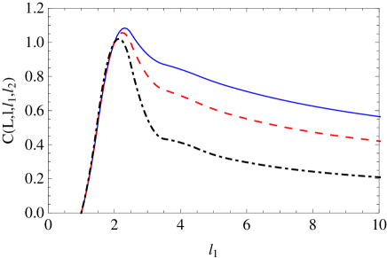
(a)  Case 1: Plot of $C(L,\ell,\ell_{1},\ell_{2})$ for $\tilde{\Delta}_{11}^{LM}(k,\tau_{s})$; with initial SH multipoles $\;\ell_{3}=\ell_{4}=1$, the final SH multipoles being $\ell=\ell_{1}-1(=\ell_{2}-1)$ and the index of deviation from statistical isotropy $L=0$ (blue, solid), $L=1$ (red, dashed) and $L=2$ (black, dot-dashed) respectively.

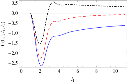
(b)  Case 2: Plot of $C(L,\ell,\ell_{1},\ell_{2})$ for $\tilde{\Delta}_{22}^{LM}(k,\tau_{s})$; with initial multipoles $\;\ell_{3}=\ell_{4}=2$, the final multipoles being $\ell=\ell_{1}(=\ell_{2})$ and the index of deviation from statistical isotropy $L=0$ (blue, solid), $L=1$ (red, dashed) and $L=2$ (black, dot-dashed) respectively.

Figure 1: Evolution of the coefficient of the spherical Bessel functions, $C(L,\ell,\ell_{1},\ell_{2})$ with multipole moment $\ell_{1}$ as in equation (41), for non-zero diagonal terms of a unit normalized $\tilde{\Delta}_{\ell_{3}\ell_{4}}^{LM}(k,\tau_{s})$

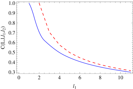
(a)  Case 1: Plot of $C(L,\ell,\ell_{1},\ell_{2})$ for $\tilde{\Delta}_{10}^{LM}(k,\tau_{s})$; with initial multipoles $\;\ell_{3}=1,\;\ell_{4}=0$, the final multipoles being $\ell=\ell_{2}=\ell_{1}+1$ (blue, solid) and $\ell=\ell_{2}=\ell_{1}-1$ (red, dashed) respectively. The terms are non-zero only when the index of deviation from statistical isotropy $L=|\ell_{3}-\ell_{4}|=1$.

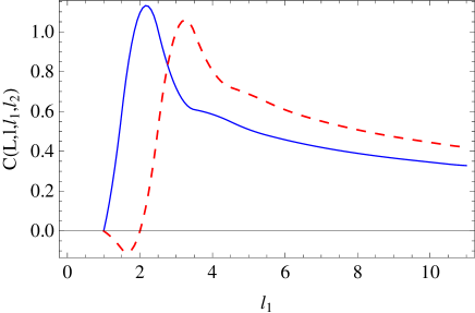
(b)  Case 2: Plot of $C(L,\ell,\ell_{1},\ell_{2})$ for $\tilde{\Delta}_{20}^{LM}(k,\tau_{s})$; with initial multipoles $\;\ell_{3}=2,\;\ell_{4}=0$, the final multipoles being $\ell=\ell_{2}=\ell_{1}$ (blue, solid) and $\ell=\ell_{2}=\ell_{1}-2$ (red, dashed) respectively. The terms are non-zero only when the index of deviation from statistical isotropy $L=|\ell_{3}-\ell_{4}|=2$.

Figure 2: Evolution of the coefficient of the spherical Bessel functions, $C(L,\ell,\ell_{1},\ell_{2})$ with multipole moment $\ell_{1}$ as in equation (41), for non-zero off-diagonal terms of a unit normalized $\tilde{\Delta}_{\ell_{3}\ell_{4}}^{LM}(k,\tau_{s})$

Setting $L=0,M=0$ we recover the statistical isotropic case as in equation (10), section (II.4).

The transfer of power of the statistical anisotropic terms to higher SH multipoles $\ell_{1}$ & $\ell_{2}$ due to free streaming is illustrated in figures (1) and (2). Starting from a unit normalized $\tilde{\Delta}_{\ell_{3},\ell_{4}}^{LM}(k,\tau_{s})$, we plot the evolution of the coefficients in equation (44), $C(L,\ell,\ell_{1},\ell_{2})$ with $\ell_{1}$ for specific values of the SH multipole moments $\ell_{3}$ and $\ell_{4}$. We find that the values of $\ell$ and $\ell_{2}$ are constrained by the values of $\ell_{1}$ due to the triangular inequalities of the Clebsch-Gordon coefficients.

Figure 1 shows the evolution of these coefficients for diagonal, unit normalized CMB brightness fluctuations namely $\tilde{\Delta}_{11}^{LM}(k,\tau_{s})$ and $\tilde{\Delta}_{22}^{LM}(k,\tau_{s})$ with $L=0,1,2$, for possible values of $\ell$ and $\ell_{2}$.

Figure 2 shows the evolution of the coefficients for off-diagonal, unit normalized $\tilde{\Delta}_{10}^{LM}(k,\tau_{s})$ and $\tilde{\Delta}_{20}^{LM}(k,\tau_{s})$, for possible values of $L,\ell$ and $\ell_{2}$. The coefficients for off-diagonal $\tilde{\Delta}_{\ell_{3},\ell_{4}}^{LM}(k,\tau_{s})$ vanish for $L=0$ i.e. the statistical isotropic case.

IV.2 SI violation at large multipoles

The ability to measure violation of statistical isotropy at low SH multipoles is largely compromised by cosmic variance. At larger SH multipoles, the effect due to violation of SI would become prominent. The previous section shows that power is transferred from small to large SH multipoles during free-streaming. This opens the door to more readily measurable SI violations arising from SI violation induced due to physical processes (e.g., presence of magnetic fields,or, other breakdown of rotational symmetries) in the baryon-photon plasma.

Due to the tight coupling in the baryon-photon plasma prior to $\tau_{s}$, primordial SI violation can be expected to be limited to small SH multipoles. It is illuminating then to obtain an expression for the free-streaming of BipoSH brightness fluctuations at small SH multipole moments at the last scattering to large SH multipoles at the present epoch for which we essentially evaluate the asymptotic limit of the CMB brightness fluctuations today.

In equation (41) we take $\ell_{1}$ & $\ell_{2}$ to be large compared to $\ell_{3}$ & $\ell_{4}$. From symmetry of Wigner-6j symbols

$$\left\{\begin{array}[]{ccc}\ell_{1}&\ell&\ell_{3}\\ \ell_{4}&L&\ell_{2}\end{array}\right\}=\left\{\begin{array}[]{ccc}\ell_{4}&L&\ell_{3}\\ \ell_{1}&\ell&\ell_{2}\end{array}\right\}.$$ (45)

We evaluate the asymptotic limit with arbitrary values of $\ell$, $\ell_{1}$, $\ell_{2}$, $\ell_{3}$ and $\ell_{4}$ using equation (9.9.1) from Varshalovich et al. (1988) as,

$$\left\{\begin{array}[]{ccc}\ell_{4}&L&\ell_{3}\\ R+d&R+e&R+f\end{array}\right\} \approx \frac{(-1)^{\ell_{4}+L+d+e}}{\sqrt{2\ell}\>\Pi_{\ell_{3}}}$$ (48)

$$\times \mathcal{C}^{\ell_{3}(d-e)}_{\ell_{4}(f-e)L(d-f)}$$ (49)

where $R$ is large and

$$d = \ell_{1}-R$$

$$e = \ell-R$$

$$f = \ell_{2}-R.$$

Thus for $\ell_{1},\ell_{2}>>\ell_{3},\ell_{4}$, equation (49) becomes

$$\left\{\begin{array}[]{ccc}\ell_{4}&L&\ell_{3}\\ \ell_{1}&\ell&\ell_{2}\end{array}\right\}\approx\frac{(-1)^{\ell_{4}+L+\ell_{1}+\ell-2R}}{\sqrt{2\ell}\>\Pi_{\ell_{3}}}\mathcal{C}^{\ell_{3}(\ell_{1}-\ell)}_{\ell_{4}(\ell_{2}-\ell)L(\ell_{1}-\ell_{2})}.$$ (50)

Putting the expression for the Wigner-6j symbols from equation (50), the asymptotic limit of the generalized evolution equation (41) takes the form

$$\tilde{\Delta}_{\ell_{1}\ell_{2}}^{LM}(k,\tau) = \sum_{\ell\ell_{3}\ell_{4}}(-i)^{\ell}\;\frac{\Pi_{\ell\ell\ell_{1}\ell_{4}}}{\sqrt{2\ell}\Pi_{\ell_{3}}}\frac{\beta_{\ell_{3}\ell_{4}}}{\beta_{\ell_{1}\ell_{2}}}\;(-1)^{\ell+\ell_{1}+\ell_{3}}$$ (51)

$$\times j_{\ell}(k\Delta\tau)\tilde{\Delta}_{\ell_{3}\ell_{4}}^{LM}(k,\tau_{s})\;\mathcal{C}^{\ell_{3}0}_{\ell 0\ell_{1}0}\;\mathcal{C}^{\ell_{2}0}_{\ell 0\ell_{4}0}$$

$$\times \mathcal{C}^{\ell_{3}(\ell_{1}-\ell)}_{\ell_{4}(\ell_{2}-\ell)L(\ell_{1}-\ell_{2})}\,.$$

Equation (51) depicts how power in SI violating terms at small SH multipoles $\ell_{3},\ell_{4}$ at the last scattering, free stream to higher SH multipoles $\ell_{1},\ell_{2}$ at the present epoch. Note the structural similarity to equation (10) for statistical isotropic case.

It is useful to provide explicit expressions for equation (51) in two particular cases, when the asymptotic moments of the CMB brightness fluctuation contains only diagonal terms and off-diagonal terms respectively.

The evolution equation which involves only the diagonal terms of the moments of the brightness fluctuation at last scattering are

$$\tilde{\Delta}_{\ell_{1},\ell_{1}}^{LM}(k,\tau) = \sum_{\ell}C_{1}(L,\ell,\ell_{1})\;j_{\ell}(k\Delta\tau)$$ (52)

$$\times \tilde{\Delta}_{\ell_{1}-\ell,\;\ell_{1}-\ell}^{LM}(k,\tau_{s})\;\;,$$

with

$$C_{1}(L,\ell,\ell_{1}) = \frac{\Pi_{\ell\ell\ell_{1}\ell_{3}}}{\sqrt{2\ell}}\left[\frac{\ell_{1}!}{\ell!\ell_{3}!}\right]^{2}\frac{(2\ell)!(2\ell_{3}+1)!}{(2\ell_{1}+1)!}\;\delta_{\ell_{3},\ell_{1}-\ell}$$ (53)

$$\times \sqrt{\frac{(2\ell_{3})!}{(2\ell_{3}-L)!}\frac{(2\ell_{3})!}{(2\ell_{3}+L+1)!}}$$

where $\ell,\ell_{1}>>|\ell_{1}-\ell|$. The details are given in Appendix C. The term under the square-root captures the $L$ dependence of the free-streaming of $L>0$ terms.

The evolution equation which involves only the off-diagonal terms of the moments of the brightness fluctuation at last scattering are

$$\tilde{\Delta}_{\ell_{1},\ell_{2}}^{LM}(k,\tau) = \sum_{\ell}C_{2}(\ell,\ell_{1},\ell_{2})\>j_{\ell}(k\Delta\tau)$$ (54)

$$\times \tilde{\Delta}_{\ell_{1}-\ell,\ell_{2}-\ell}^{LM}(k,\tau_{s})\delta_{L,\ell_{1}-\ell_{2}},$$

with

$$C_{2}(\ell,\ell_{1},\ell_{2}) = \frac{(-1)^{\frac{\ell_{1}+\ell_{2}}{2}}}{\sqrt{2\ell}}\frac{\Pi_{\ell\ell\ell_{1}\ell_{2}}}{\Pi_{\ell_{1}-\ell}}\>\sqrt{\frac{\ell_{1}+\ell_{2}-2\ell+1}{\ell_{1}+\ell_{2}+1}}$$ (55)

$$\times \frac{(2\ell)!\ell_{1}!\ell_{2}!}{(\ell!)^{2}(\ell_{1}-\ell)!(\ell_{2}-\ell)!}$$

$$\times \left[\frac{(2\ell_{1}-2\ell+1)!(2\ell_{2}-2\ell+1)!}{(2\ell_{1}+1)!(2\ell_{2}+1)!}\right]^{\frac{1}{2}}.$$

where $\ell,\;\ell_{n}>>|\ell_{n}-\ell|,\;L$ with $n=1,2$. The details are given in Appendix D. As in equation (53), the term under the square-root captures the $L$ dependence of the free-streaming of $L>0$ terms.

IV.3 SI violating physical effects at last scattering

The patterns of the CMB temperature field i.e. the angular correlations observed today are traced back to inhomogeneities at the last scattering surface. In the tight coupling regime of the baryon-photon fluid, one expects power only at small SH multipoles of the $\tilde{\Delta}_{\ell_{1}\ell_{2}}^{LM}(k,\tau_{s})$. The generalized evolution equation of the CMB brightness fluctuations (36) free-streams this power at small SH multipoles in both SI and non-SI moments to corresponding SI and non-SI moments with same Bipolar moment $L$. Any observed violation of SI today is easier to interpret as generalized moments arising due to simple physics just beyond the fluid approximation regime. In this section, we illustrate this point explicitly for SI violation in the CMB anisotropy in the presence of a homogeneous magnetic field at last scattering.

The SH coefficients $a_{\ell m}$ can be expressed in terms of the CMB brightness fluctuations at last scattering using equation (13) and the generalized evolution equation (41) as

$$a_{\ell m} = 4\pi\int\frac{d^{3}k}{(2\pi)^{3}}\;\phi(\vec{k})\sum_{\ell_{1}m_{1}LM}\beta_{\ell_{1}\ell}\;\mathcal{C}^{LM}_{\ell_{1}m_{1}\ell m}\;Y_{\ell_{1}m_{1}}(\hat{k})$$ (56)

$$\times \sum_{\ell_{2}\ell_{3}\ell_{4}}C(L,\ell_{2},\ell_{1},\ell)\;j_{\ell_{2}}(k\Delta\tau)\;\tilde{\Delta}_{\ell_{3}\ell_{4}}^{LM}(k,\tau_{s}),$$

where $C(L,\ell_{2},\ell_{1},\ell)$ is defined in equation (44).

Hence, in general $\langle a_{\ell m}a_{\ell^{\prime}m^{\prime}}\rangle$ correlations measured at present are related to $\langle\tilde{\Delta}_{\ell_{1}\ell_{2}}^{LM}(k,\tau_{s})\tilde{\Delta}_{\ell_{3}\ell_{4}}^{L^{\prime}M^{\prime}}(k,\tau_{s})\rangle$ correlation between the generalized Boltzmann fluctuations at the last scattering surface.

In particular, SI violation encoded in the off-diagonal correlation $\langle a_{\ell m}a_{\ell^{\prime}m^{\prime}}\rangle$ (and non-zero BipoSH $A^{LM}_{\ell\ell^{\prime}}$, $L>0$) are related as

$$A^{JN}_{\ell\ell^{\prime}}\sim\left\{\tilde{\Delta}^{L}_{\ell_{1}\ell}(k,\tau_{s})\otimes\tilde{\Delta}^{L^{\prime}}_{\ell_{2}\ell^{\prime}}(k,\tau_{s})\right\}_{JN}$$ (57)

as in equations (31, 32, 33) or more generally for different Bipolar coefficients $J^{\prime}$ and $N^{\prime}$ as in equation (26) when the power spectrum is also anisotropic.

Using equation (11), correlations of the CMB brightness fluctuations are

$$\langle\Delta(\vec{k},\hat{n},\tau_{s})\Delta(\vec{k},\hat{n^{\prime}},\tau_{s})\rangle\!\! = \!\!(4\pi)^{2}\!\!\sum_{\ell_{1}\ell_{2}LM}\sum_{\ell_{3}\ell_{4}L^{\prime}M^{\prime}}\beta_{\ell_{1}\ell_{2}}\;\beta_{\ell_{3}\ell_{4}}$$ (58)

$$\times \tilde{\Delta}^{LM}_{\ell_{1}\ell_{2}}(k,\tau_{s})\tilde{\Delta}^{L^{\prime}M^{\prime}}_{\ell_{3}\ell_{4}}(k,\tau_{s})$$

$$\times \left\{Y_{\ell_{1}}(\hat{k})\otimes Y_{\ell_{2}}(\hat{n})\right\}_{LM}$$

$$\times \left\{Y_{\ell_{3}}(\hat{k})\otimes Y_{\ell_{4}}(\hat{n^{\prime}})\right\}_{L^{\prime}M^{\prime}}.$$

We illustrate the generality and power of our formalism using the case for a uniform magnetic field. We show the correlations of the CMB brightness fluctuations in this particular case is sourced by the bipolar dipole ($L=1$) terms of equation (11) with $\ell_{1}=\ell_{2}=1$ where

$$\Delta(\vec{k},\hat{n},\tau_{s})\! = 4\pi i\sqrt{3}\sum_{M}\tilde{\Delta}^{1M}_{11}(k,\tau_{s})\left\{Y_{1}(\hat{k})\otimes Y_{1}(\hat{n})\right\}_{1M}$$ (59)

$$= 3i\sqrt{\frac{3}{2}}\sum_{M}\tilde{\Delta}^{1M}_{11}(k,\tau_{s})\;\;(\hat{k}\bm{\times}\hat{n})_{M},$$

with $M=\{-1,0,+1\}$. Here $(\hat{k}\bm{\times}\hat{n})_{M}$ is the usual cross-product written as irreducible products of the rotation group Varshalovich et al. (1988).

Using standard vector identity Varshalovich et al. (1988) and equation (8)

$$(\hat{n}\cdot\hat{n^{\prime}})(\hat{k}\cdot\hat{k}) - (\hat{n}\cdot\hat{k})(\hat{n^{\prime}}\cdot\hat{k})$$ (60)

$$= (\hat{n}\bm{\times}\hat{k})\cdot(\hat{n^{\prime}}\bm{\times}\hat{k}),$$

the temperature correlations in presence of a uniform magnetic field as discussed in Durrer et al. (1998) (see equation A3) are given by

$$\langle\Delta(\vec{k},\hat{n},\tau_{s})\Delta(\vec{k},\hat{n^{\prime}},\tau_{s})\rangle \propto \tilde{\Delta}^{1M}_{11}(k,\tau_{s})\;\;\tilde{\Delta}^{1M^{\prime}}_{11}(k,\tau_{s})$$ (61)

$$\times (\hat{n}\bm{\times}\hat{k})\cdot(\hat{n^{\prime}}\bm{\times}\hat{k}).$$

Here the bipolar dipole terms of the CMB brightness fluctuation $\tilde{\Delta}^{1M}_{11}(k,\tau_{s})\;\tilde{\Delta}^{1M^{\prime}}_{11}(k,\tau_{s})$ in equation (59), encapsulates the source term due to the presence of a uniform magnetic field Durrer et al. (1998).

In equation (56), the bipolar dipole terms $\tilde{\Delta}_{11}^{1M}(k,\tau_{s})$ gives rise to SH coefficients

$$a_{\ell m} = 4\pi\int\frac{d^{3}k}{(2\pi)^{3}}\;\phi(\vec{k})\sum_{m_{1}M}\beta_{1\ell}\;\mathcal{C}^{1M}_{1m_{1}\ell m}\;Y_{1m_{1}}(\hat{k})$$ (62)

$$\times \sum_{\ell_{3}}\left[(...)j_{\ell-1}(k\Delta\tau)+(...)j_{\ell+1}(k\Delta\tau)\right]$$

$$\times \tilde{\Delta}_{11}^{1M}(k,\tau_{s}).$$

The angular correlations in this case turn out to be

$$\langle a_{\ell m}a^{*}_{\ell^{\prime}m^{\prime}}\rangle = (...)\;\delta_{\ell^{\prime}\ell}\delta_{mm^{\prime}}+(...)\;\delta_{\ell^{\prime}\>\ell\pm 2}\delta_{mm^{\prime}}.$$ (63)

It is interesting to note that the known diagonal ($\ell^{\prime}=\ell$) and off-diagonal ($\ell^{\prime}=\ell\pm 2$) correlations in presence of a homogeneous magnetic field Durrer et al. (1998); Kahniashvili et al. (2008), can be easily recovered in our approach. Work is in progress to relate other cases of SI violation originating in the physics at the last scattering surface using this formalism.

V Conclusions

The search for subtle statistical isotropy breakdown in the universe is highly motivated by numerous theoretical scenarios. The fluctuations in the cosmic microwave background is the arguably the most promising observational probe of the SI of the universe. The violation of SI could have its origin not only in in anisotropic primordial power spectrum, but also in the SI violation in the fluctuations of the baryon-photon fluid at last scattering. SI deviations generated by a general form of anisotropic primordial power spectrum for isotropic Boltzmann functions has been studied in the recent literature Pullen and Kamionkowski (2007). This paper includes this equally important possibility of a general SI breakdown in the CMB photon distribution function. We study the generalized case of SI violation in terms of Bipolar spherical harmonic (BipoSH) brightness fluctuations, substantially extending the scope of origin of SI violation solely from the anisotropic primordial power spectrum.

The breakdown of SI in the CMB brightness fluctuation results in off-diagonal terms in the SH space angular correlations $\langle a_{\ell m}a_{\ell^{\prime}m^{\prime}}\rangle$, or, equivalently, in the coefficients the Bipolar spherical harmonic (BipoSH) representation Hajian and Souradeep (2004, 2006). We relate the measurable BipoSH coefficients to SI deviations in the baryon-photon fluid, as well as, the primordial power spectrum. The observable BipoSH coefficients can be compactly expressed in terms BipoSH brightness fluctuations terms through products of standard Clebsch-Gordon coefficients and a Wigner-9j function. We also present the expression for the simpler case of an isotropic primordial power spectrum, where the BipoSH coefficients turn out to be given through a compact combination of a Wigner-6j symbol and a Clebsch-Gordon coefficient. We also provide the large SH multipole limit for these coefficients for the terms encoding deviations from SI at low BipoSH multipoles.

We obtain the generalized free-stream evolution equation for the SI violation encoded in terms of the BipoSH brightness fluctuations introduced in our work. We demonstrate that different modes BipoSH brightness fluctuations at the present epoch have to evolve from same Bipolar modes at the last scattering. The moments of the CMB brightness fluctuations $\tilde{\Delta}^{LM}_{\ell_{1}\ell_{2}}(\hat{k},\tau_{s})$ at last scattering are expected to non-zero at small values of SH multipoles $\ell_{1}$ and $\ell_{2}$ due to tight coupling. However, our results show that the power in these SI violating terms at low SH multipoles would be transferred during free-stream evolution to higher multipoles $\ell_{3}$ and $\ell_{4}$ in $\tilde{\Delta}^{LM}_{\ell_{3}\ell_{4}}(\hat{k},\tau)$ at the present epoch. This is akin to the well known free-streaming evolution of power in the SI brightness fluctuation at low SH multipole power at last scattering to large SH multipole at present. For clearly highlighting the structural similarity, we present the evolution of BipoSH brightness fluctuations in the asymptotic case of large values of the final SH multipoles today relative to the initial SH multipoles at last scattering.

While many of the claimed observational evidence of SI breakdown, such as the “axis of evil”, “north-south asymmetry” etc., pertain to relatively small values of the SH multipoles where the significance is largely obscured by dominance of cosmic variance. However, SI violation at small SH multipoles in the baryon-photon plasma at last scattering would free-stream to large SH multipoles at present, and consequently, would be easier to establish from CMB observations. A program of study to relate the BipoSH brightness fluctuations in the baryon-photon fluid for different physical scenarios is currently underway. We have used our formalism to represent and match the well known case for SI violation in presence of a homogeneous magnetic field. We illustrate how the angular correlations in such a case could be seeded by the dipole term of the generalized CMB brightness fluctuation and would have diagonal ($\ell^{\prime}=\ell$) and off-diagonal ($\ell^{\prime}=\ell\pm 2$) terms.

In summary, our work strongly motivates closer study of all possible SI violating phenomena and scenarios in the simple baryon-photon plasma, since these could potentially provide more readily observable signature of SI violation in the universe. It is also encouraging that it may have observational implications in light of the recent WMAP-7 discovery Bennett et al. (2010). Since, the quadrupolar anisotropy anomaly with non-zero BipoSH coefficients related as $A_{\ell\ell}^{2M}\sim-2A_{\ell-2\ell}^{2M}$, rule out an origin in anisotropic power spectrum, this may well be related to SI violations in the CMB brightness fluctuations. This possibility is also bolstered by the fact that the non-SI effect peaks at acoustic $l\sim 200$ scales pointing to some non-trivial physics at the last scattering surface. Extension of this formalism to CMB polarization should be readily possible. The formalism and the initial conclusions are important and timely in light of higher precision and resolution CMB anisotropy and polarization data expected in near future, in particular, from the ongoing Planck Surveyor CMB mission.

Appendix A Bipolar coefficients for SI deviations

The BipoSH coefficients are defined in equation (19). For a directional dependent primordial power spectrum as in equation (16), these Bipolar coefficients can be evaluated using the angular correlations in equation (17) in the following way

$$A^{JN}_{\ell\ell^{\prime}}=\left(A^{JN}_{\ell\ell^{\prime}}\right)_{\mathfrak{l}=0} + \sqrt{4\pi}\int\frac{k^{2}dk}{2\pi^{2}}P_{0}(k)\sum_{\mathfrak{l}\ell_{1}\ell_{2}LL^{\prime}}\frac{\Pi_{\ell_{1}\ell_{3}}}{\Pi_{\ell_{2}}}\beta_{\ell_{1}\ell}\beta_{\ell_{2}\ell^{\prime}}^{*}\mathcal{C}^{\ell_{2}0}_{\ell_{1}0\mathfrak{l}0}\sum_{\mathfrak{m}}g_{\mathfrak{l}\mathfrak{m}}\sum_{MM^{\prime}}\tilde{\Delta}_{\ell_{1}\ell}^{LM}(k,\tau)\;[\tilde{\Delta}_{\ell_{2}\ell^{\prime}}^{L^{\prime}M^{\prime}}(k,\tau)]^{*}$$ (64)

$$\times \sum_{m_{1}m_{2}mm^{\prime}}(-1)^{m^{\prime}}\mathcal{C}^{LM}_{\ell_{1}m_{1}\ell m}\mathcal{C}^{L^{\prime}M^{\prime}}_{\ell_{2}m_{2}\ell^{\prime}m^{\prime}}\mathcal{C}^{JN}_{\ell m\ell^{\prime}-m^{\prime}}\mathcal{C}^{\ell_{2}m_{2}}_{\ell_{1}m_{1}\mathfrak{l}\mathfrak{m}}.$$

We use the following symmetry properties of the Clebsch-Gordan coefficients in equation (8.4.10) from Varshalovich et al. (1988)

$$\mathcal{C}^{\ell_{2}m_{2}}_{\ell_{1}m_{1}\mathfrak{l}\mathfrak{n}} = (-1)^{\mathfrak{l}+\ell_{1}-\ell_{2}}\mathcal{C}^{\ell_{2}-m_{2}}_{\ell_{1}-m_{1}\mathfrak{l}-\mathfrak{m}}$$ (65)

$$= (-1)^{\ell_{1}-\ell_{2}}\frac{\Pi_{\ell_{2}}}{\Pi_{\ell_{1}}}(-1)^{\mathfrak{m}}\mathcal{C}^{\ell_{1}m_{1}}_{\ell_{2}m_{2}\mathfrak{l}-\mathfrak{m}}$$

and

$$\mathcal{C}^{JN}_{\ell m\ell^{\prime}-m^{\prime}} = (-1)^{\ell^{\prime}-m^{\prime}}\frac{\Pi_{J}}{\Pi_{\ell}}\mathcal{C}^{\ell m}_{\ell^{\prime}m^{\prime}JN},$$ (66)

where $\Pi_{\ell_{1}\ell_{2}...\ell_{n}}=[(2\ell_{1}+1)(2\ell_{2}+1)...(2\ell_{n}+1)]^{\frac{1}{2}}$ has been defined for convenient notational simplicity.
We use the formula for summation of the product of four Clebsch-Gordan coefficients given in equation (8.7.26) from Varshalovich et al. (1988)

$$\sum_{m_{1}m_{2}mm^{\prime}}\mathcal{C}^{LM}_{\ell_{1}m_{1}\ell m}\mathcal{C}^{L^{\prime}M^{\prime}}_{\ell_{2}m_{2}\ell^{\prime}m^{\prime}}\mathcal{C}^{\ell m}_{\ell^{\prime}m^{\prime}JN}\mathcal{C}^{\ell_{1}m_{1}}_{\ell_{2}m_{2}\mathfrak{l}-\mathfrak{m}}=\sum_{\ell_{3}m_{3}}\Pi_{\ell\ell_{1}L^{\prime}\ell_{3}}\mathcal{C}^{\ell_{3}m_{3}}_{L^{\prime}M^{\prime}JN}\mathcal{C}^{LM}_{L^{\prime}M^{\prime}\ell_{3}m_{3}}\left\{\begin{array}[]{ccc}\!L\!&\ell_{1}\!&\ell\!\\ \!L^{\prime}\!&\ell_{2}\!&\ell^{\prime}\!\\ \!\ell_{3}\!&\mathfrak{l}\!&J\!\end{array}\right\}\;.$$ (70)

The Bipolar coefficients in equation (64) simplifies to

$$A^{JN}_{\ell\ell^{\prime}}=\left(A^{JN}_{\ell\ell^{\prime}}\right)_{\mathfrak{l}=0} + \sqrt{4\pi}\int\frac{k^{2}dk}{2\pi^{2}}P_{0}(k)\sum_{\mathfrak{l}\ell_{1}\ell_{2}LL^{\prime}}\Pi_{\mathfrak{l}\ell_{1}LL^{\prime}}(-1)^{\mathfrak{l}+L^{\prime}+\ell^{\prime}+\ell_{1}-\ell_{2}}\>\beta_{\ell_{1}\ell}\>\beta_{\ell_{2}\ell^{\prime}}^{*}\>\mathcal{C}^{\ell_{2}0}_{\ell_{1}0\mathfrak{l}0}$$ (74)

$$\times \sum_{\mathfrak{l}}g_{\mathfrak{l}\mathfrak{m}}\sum_{\ell_{3}m_{3}}\left\{\begin{array}[]{ccc}\!J\!&\ell_{3}\!&\mathfrak{l}\!\\ \!\ell\!&L\!&\ell_{1}\!\\ \!\ell^{\prime}\!&L^{\prime}\!&\ell_{2}\!\end{array}\right\}\>\mathcal{C}^{JN}_{\ell_{3}m_{3}\mathfrak{l}\mathfrak{m}}\left\{\tilde{\Delta}^{L}_{\ell_{1}\ell}\otimes\tilde{\Delta}^{L^{\prime}}_{\ell_{2}\ell^{\prime}}\right\}_{\ell_{3}m_{3}}.$$

$\{\tilde{\Delta}^{L}_{\ell_{1}\ell}\otimes\tilde{\Delta}^{L^{\prime}}_{\ell_{1}\ell^{\prime}}\}_{JN}$ are the Bipolar products in $L$ and $L^{\prime}$ as defined in equation (21).

For statistically isotropic primordial perturbations, the angular correlation in equation (27) can be written in terms of Bipolar coefficients as

$$(A^{JN}_{\ell\ell^{\prime}})_{\mathfrak{l}=0} = 4\pi\int\frac{k^{2}dk}{2\pi^{2}}P_{0}(k)\sum_{\ell_{1}LL^{\prime}}\beta_{\ell_{1}\ell}\>\>\beta_{\ell_{1}\ell^{\prime}}^{*}\sum_{MM^{\prime}}\tilde{\Delta}_{\ell_{1}\ell}^{LM}(k,\tau)\>\>[\tilde{\Delta}_{\ell_{1}\ell^{\prime}}^{L^{\prime}M^{\prime}}(k,\tau)]^{*}$$ (75)

$$\times \sum_{m_{1}mm^{\prime}}(-1)^{m^{\prime}}\mathcal{C}^{JN}_{\ell m\ell^{\prime}-m^{\prime}}\mathcal{C}^{LM}_{\ell_{1}m_{1}\ell m}\mathcal{C}^{L^{\prime}M^{\prime}}_{\ell_{1}m_{1}\ell^{\prime}m^{\prime}}.$$

The summation in the above equation can be simplified using equation (8.7.17) from Varshalovich et al. (1988) as follows

$$\sum_{m_{1}mm^{\prime}}(-1)^{m^{\prime}}\mathcal{C}^{JN}_{\ell m\ell^{\prime}-m^{\prime}}\mathcal{C}^{LM}_{\ell_{1}m_{1}\ell m}\mathcal{C}^{L^{\prime}M^{\prime}}_{\ell_{1}m_{1}\ell^{\prime}m^{\prime}} = (-1)^{\ell_{1}+L+J}\>\Pi_{L^{\prime}\mathcal{L^{\prime\prime}}}\mathcal{C}^{LM}_{L^{\prime}M^{\prime}JN}\left\{\begin{array}[]{ccc}\ell^{\prime}&\ell_{1}&L^{\prime}\\ L&J&\ell\end{array}\right\}$$ (78)

$$= (-1)^{\ell_{1}+L+J}\>\Pi_{L^{\prime}\mathcal{L^{\prime\prime}}}(-1)^{L^{\prime}-M^{\prime}}\>\frac{\Pi_{L}}{\Pi_{J}}\mathcal{C}^{JN}_{LML^{\prime}-M^{\prime}}\left\{\begin{array}[]{ccc}L&J&L^{\prime}\\ \ell^{\prime}&\ell_{1}&\ell\end{array}\right\}$$ (81)

$$= (-1)^{\ell_{1}+L+L^{\prime}+J}\>\Pi_{LL^{\prime}}(-1)^{M^{\prime}}\mathcal{C}^{JN}_{LML^{\prime}-M^{\prime}}\>\left\{\begin{array}[]{ccc}L&J&L^{\prime}\\ \ell^{\prime}&\ell_{1}&\ell\end{array}\right\}\;.$$ (84)

Thus the BipoSH coefficient can be simplified to

$$(A^{JN}_{\ell\ell^{\prime}})_{\mathfrak{l}=0} = 4\pi\int\frac{k^{2}dk}{2\pi^{2}}P_{0}(k)\sum_{\ell_{1}LL^{\prime}}(-1)^{\ell_{1}+L+L^{\prime}+J}\>\Pi_{LL^{\prime}}\beta_{\ell_{1}\ell}\>\>\beta_{\ell_{1}\ell^{\prime}}^{*}\left\{\begin{array}[]{ccc}L&J&L^{\prime}\\ \ell^{\prime}&\ell_{1}&\ell\end{array}\right\}$$

$$\times \sum_{MM^{\prime}}\tilde{\Delta}_{\ell_{1}\ell}^{LM}(k,\tau)\>\>[\tilde{\Delta}_{\ell_{1}\ell^{\prime}}^{L^{\prime}M^{\prime}}(k,\tau)]^{*}(-1)^{M^{\prime}}\mathcal{C}^{JN}_{LML^{\prime}-M^{\prime}}$$

$$= 4\pi\int\frac{k^{2}dk}{2\pi^{2}}P_{0}(k)\sum_{\ell_{1}LL^{\prime}}(-1)^{\ell_{1}+L+L^{\prime}+J}\>\Pi_{LL^{\prime}}\beta_{\ell_{1}\ell}\>\>\beta_{\ell_{1}\ell^{\prime}}^{*}\left\{\begin{array}[]{ccc}L&J&L^{\prime}\\ \ell^{\prime}&\ell_{1}&\ell\end{array}\right\}$$ (90)

$$\times \left\{\tilde{\Delta}^{L}_{\ell_{1}\ell}\otimes\tilde{\Delta}^{L^{\prime}}_{\ell_{1}\ell^{\prime}}\right\}_{JN}\;,$$ (91)

where symmetry properties of the Clebsch-Gordan coefficients, equations (8.4.10) in Varshalovich et al. (1988) has been used. To consider low Bipolar deviations from statistical isotropy i.e. $(L,L^{\prime},J<<\ell,\ell^{\prime},\ell_{1})$, we use the asymptotic relation for Wigner-6j function as given in equation (9.9.1) from Varshalovich et al. (1988)

$$\left\{\begin{array}[]{ccc}L&J&L^{\prime}\\ \ell^{\prime}&\ell_{1}&\ell\end{array}\right\} \approx \frac{(-1)^{L+J+\ell^{\prime}-\ell_{1}}}{\sqrt{2\ell_{1}}\;\Pi_{L^{\prime}}}\mathcal{C}^{L^{\prime}(\ell^{\prime}-\ell_{1})}_{L(\ell-\ell_{1})J(\ell^{\prime}-\ell)}$$ (94)

$$\approx \frac{(-1)^{J+\ell+\ell^{\prime}}}{\sqrt{2\ell_{1}}\;\Pi_{J}}\mathcal{C}^{J(\ell-\ell^{\prime})}_{L(\ell-\ell_{1})L^{\prime}(\ell_{1}-\ell^{\prime})}.$$ (95)

Using the above relation, the asymptotic limit to the BipoSH coefficients turn out to be

$$(A^{JN}_{\ell\ell^{\prime}})_{\mathfrak{l}=0} \approx \!4\pi\!\int\frac{k^{2}dk}{2\pi^{2}}P_{0}(k)\!\sum_{\ell_{1}LL^{\prime}}(-1)^{\ell+\ell^{\prime}+\ell_{1}+L+L^{\prime}}\!\frac{\Pi_{LL^{\prime}}}{\sqrt{2\ell_{1}}\>\Pi_{J}}\>\beta_{\ell_{1}\ell}\>\beta_{\ell_{1}\ell^{\prime}}^{*}\>\mathcal{C}^{J(\ell-\ell^{\prime})}_{L(\ell-\ell_{1})L^{\prime}(\ell_{1}-\ell^{\prime})}\left\{\tilde{\Delta}^{L}_{\ell_{1}\ell}\otimes\tilde{\Delta}^{L^{\prime}}_{\ell_{1}\ell^{\prime}}\right\}_{JN}\!.$$ (96)

Appendix B Generalized evolution equation for statistical isotropy breakdown

Starting with equation (36), putting $P_{\ell}(\hat{k}\cdot\hat{n})=\frac{4\pi}{2\ell+1}\sum_{m}Y_{\ell m}^{*}(\hat{k})\>Y_{\ell m}(\hat{n})$ and evaluating the double integral using the equation

$$\int d\Omega_{\hat{n}}Y_{\ell m}(\hat{n})\;Y_{\ell_{1}m_{1}}(\hat{n})Y_{\ell_{2}m_{2}}(\hat{n})^{*}=\frac{1}{\sqrt{4\pi}}\;\frac{\Pi_{\ell\ell_{1}}}{\Pi_{\ell_{2}}}\mathcal{C}^{\ell_{2}0}_{\ell 0\ell_{1}0}\;\mathcal{C}^{\ell_{2}m_{2}}_{\ell m\ell_{1}m_{1}},$$ (97)

the most general evolution equation becomes

$$\tilde{\Delta}_{\ell_{1}\ell_{2}}^{LM}(k,\tau)=\frac{1}{\beta_{\ell_{1}\ell_{2}}}\sum_{\ell}(-i)^{\ell}\;\Pi_{\ell}^{2}\;j_{\ell}(k\Delta\tau)\sum_{\ell_{3}\ell_{4}L^{\prime}M^{\prime}}\!\!\!\!\!\!\beta_{\ell_{3}\ell_{4}}\tilde{\Delta}_{\ell_{3}\ell_{4}}^{L^{\prime}M^{\prime}}(k,\tau_{s})\frac{\Pi_{\ell_{1}\ell_{4}}}{\Pi_{\ell_{2}\ell_{3}}}\mathcal{C}_{g}\;,$$ (98)

where

$$\mathcal{C}_{g}=\mathcal{C}^{\ell_{3}0}_{\ell 0\ell_{1}0}\;\mathcal{C}^{\ell_{2}0}_{\ell 0\ell_{4}0}\sum_{m_{1}m_{2}}\mathcal{C}^{LM}_{\ell_{1}m_{1}\ell_{2}m_{2}}\sum_{m_{3}m_{4}}\mathcal{C}^{L^{\prime}M^{\prime}}_{\ell_{3}m_{3}\ell_{4}m_{4}}\sum_{m}\mathcal{C}^{\ell_{3}m_{3}}_{\ell m\ell_{1}m_{1}}\;\mathcal{C}^{\ell_{2}m_{2}}_{\ell m\ell_{4}m_{4}}.$$ (99)

Using the summation formula for four Clebsch-Gordon coefficients given by equation (9.1.8) from Varshalovich et al. (1988),

$$\sum_{mm_{1}m_{2}m_{3}m_{4}}\mathcal{C}^{L^{\prime}M^{\prime}}_{\ell_{3}m_{3}\ell_{4}m_{4}}\;\mathcal{C}^{\ell_{3}m_{3}}_{\ell_{1}m_{1}\ell m}\;\mathcal{C}^{LM}_{\ell_{1}m_{1}\ell_{2}m_{2}}\mathcal{C}^{\ell_{2}m_{2}}_{\ell m\ell_{4}m_{4}}=\delta_{L^{\prime}L}\delta_{M^{\prime}M}(-1)^{\ell_{1}+\ell+\ell_{4}+L^{\prime}}\Pi_{\ell_{2}\ell_{3}}\left\{\begin{array}[]{ccc}\ell_{1}&\ell&\ell_{3}\\ \ell_{4}&L^{\prime}&\ell_{2}\end{array}\right\}\;,$$ (100)

equation (98) simplifies to

$$\tilde{\Delta}_{\ell_{1}\ell_{2}}^{LM}(k,\tau) = \sum_{\ell\ell_{3}\ell_{4}}(-i)^{\ell}\;\Pi_{\ell\ell\ell_{1}\ell_{4}}\frac{\beta_{\ell_{3}\ell_{4}}}{\beta_{\ell_{1}\ell_{2}}}\;(-1)^{\ell_{3}+\ell_{4}+L}\;j_{\ell}(k\Delta\tau)\tilde{\Delta}_{\ell_{3}\ell_{4}}^{LM}(k,\tau_{s})\;\mathcal{C}^{\ell_{3}0}_{\ell 0\ell_{1}0}\;\mathcal{C}^{\ell_{2}0}_{\ell 0\ell_{4}0}\;\left\{\begin{array}[]{ccc}\ell_{1}&\ell&\ell_{3}\\ \ell_{4}&L&\ell_{2}\end{array}\right\}$$ (103)

$$= \sum_{\ell\ell_{3}\ell_{4}}(-i)^{\ell}\;\Pi_{\ell\ell\ell_{1}\ell_{4}}\frac{\beta_{\ell_{3}\ell_{4}}}{\beta_{\ell_{1}\ell_{2}}}\;(-1)^{\ell_{3}+\ell_{4}+L}\;j_{\ell}(k\Delta\tau)\tilde{\Delta}_{\ell_{3}\ell_{4}}^{LM}(k,\tau_{s})\;\mathcal{C}^{\ell_{3}0}_{\ell 0\ell_{1}0}\;\mathcal{C}^{\ell_{2}0}_{\ell 0\ell_{4}0}\;\left\{\begin{array}[]{ccc}\ell_{1}&L&\ell_{2}\\ \ell_{4}&\ell&\ell_{3}\end{array}\right\}.$$ (106)

Substituting the multipole dependent coefficients as

$$C(L,\ell,\ell_{1},\ell_{2})=(-i)^{\ell}\;\Pi_{\ell\ell\ell_{1}\ell_{4}}\frac{\beta_{\ell_{3}\ell_{4}}}{\beta_{\ell_{1}\ell_{2}}}\;(-1)^{\ell_{3}+\ell_{4}+L}\mathcal{C}^{\ell_{3}0}_{\ell 0\ell_{1}0}\;\mathcal{C}^{\ell_{2}0}_{\ell 0\ell_{4}0}\;\left\{\begin{array}[]{ccc}\ell_{1}&L&\ell_{2}\\ \ell_{4}&\ell&\ell_{3}\end{array}\right\}\;,$$ (107)

the generalized evolution equation for deviations of statistical isotropy in the CMB brightness fluctuation reduces to

$$\tilde{\Delta}_{\ell_{1}\ell_{2}}^{LM}(k,\tau)=\sum_{\ell\ell_{3}\ell_{4}}C(L,\ell,\ell_{1},\ell_{2})\;j_{\ell}(k\Delta\tau)\;\tilde{\Delta}_{\ell_{3}\ell_{4}}^{LM}(k,\tau_{s})\;.$$ (108)

Appendix C Diagonal terms of the asymptotic moments of CMB brightness fluctuation

In equation (49), taking $e=0$ i.e. $\ell=R$ and putting $\ell_{1}=R+\ell_{4}$ & $\ell_{2}=R+\ell_{3}$, we can write equation (50) as

$$\left\{\begin{array}[]{ccc}\ell_{4}&L&\ell_{3}\\ \ell+\ell_{4}&\ell&\ell+\ell_{3}\end{array}\right\}\approx\frac{(-1)^{L}}{\sqrt{2\ell}\>\Pi_{\ell_{3}}}\mathcal{C}^{\ell_{3}\ell_{4}}_{\ell_{4}\ell_{3}L(\ell_{4}-\ell_{3})}.$$ (109)

From the properties of the Clebsch-Gordon coefficient, we get $\ell_{3}=\ell_{4}$ and hence $\ell_{1}=\ell_{2}$. Thus in equation (41) substituting $\ell_{3}=\ell_{1}-\ell$, we get the factor

$$C_{1}(L,\ell,\ell_{1})=(-i)^{\ell}\;\Pi_{\ell}^{2}\;\Pi_{\ell_{1}}\;\Pi_{\ell_{1}-\ell}\frac{\beta_{\ell_{1}-\ell,\ell_{1}-\ell}}{\beta_{\ell_{1},\ell_{1}}}(-1)^{L}\;\mathcal{C}^{(\ell_{1}-\ell)0}_{\ell 0\ell_{1}0}\;\mathcal{C}^{\ell_{1}0}_{\ell 0(\ell_{1}-\ell)0}\frac{(-1)^{L}}{\sqrt{2\ell}\,\Pi_{\ell_{1}-\ell}}\mathcal{C}^{(\ell_{1}-\ell)(\ell_{1}-\ell)}_{(\ell_{1}-\ell)(\ell_{1}-\ell)L0}\;\;.$$ (110)

Now using equation (8.4.10) from Varshalovich et al. (1988),

$$\mathcal{C}^{(\ell_{1}-\ell)0}_{\ell 0\ell_{1}0} = (-1)^{\ell+\ell_{1}-(\ell_{1}-\ell)}\mathcal{C}^{(\ell_{1}-\ell)0}_{\ell_{1}0\ell 0}=\mathcal{C}^{(\ell_{1}-\ell)0}_{\ell_{1}0\ell 0},$$

$$\mathcal{C}^{\ell_{1}0}_{\ell 0(\ell_{1}-\ell)0} = (-1)^{\ell}\frac{\Pi_{\ell_{1}}}{\Pi_{\ell_{1}-\ell}}\mathcal{C}^{(\ell_{1}-\ell)0}_{\ell_{1}0\ell 0}.$$ (111)

Using equations (8.5.34) and (8.5.42) from Varshalovich et al. (1988), we get

$$\left[\mathcal{C}^{(\ell_{1}-\ell)0}_{\ell_{1}0\ell 0}\right]^{2}=\left[\frac{\ell_{1}!}{\ell!(\ell_{1}-\ell)!}\right]^{2}\frac{(2\ell)!(2\ell_{1}-2\ell+1)!}{(2\ell_{1}+1)!},$$ (112)

and

$$\mathcal{C}^{(\ell_{1}-\ell)(\ell_{1}-\ell)}_{(\ell_{1}-\ell)(\ell_{1}-\ell)L0}=(2\ell_{1}-2\ell)!\sqrt{\frac{2\ell_{1}-2\ell+1}{(2\ell_{1}-2\ell-L)!(2\ell_{1}-2\ell+L+1)!}}\;\;.$$ (113)

Thus

$$C_{1}(L,\ell,\ell_{1})=\frac{\Pi_{\ell}^{2}\Pi_{\ell_{1}}\Pi_{\ell_{3}}}{\sqrt{2\ell}}\left[\frac{\ell_{1}!}{\ell!\ell_{3}!}\right]^{2}\frac{(2\ell)!(2\ell_{3}+1)!}{(2\ell_{1}+1)!}\;\;\sqrt{\frac{(2\ell_{3})!}{(2\ell_{3}-L)!}\frac{(2\ell_{3})!}{(2\ell_{3}+L+1)!}}\;\;\delta_{\ell_{3},\ell_{1}-\ell}\;\;.$$ (114)

Substituting this in equation (41), the evolution equation becomes

$$\tilde{\Delta}_{\ell_{1},\ell_{1}}^{LM}(k,\tau)=\sum_{\ell}C_{1}(L,\ell,\ell_{1})\;j_{\ell}(k\Delta\tau)\;\tilde{\Delta}_{\ell_{1}-\ell,\;\ell_{1}-\ell}^{LM}(k,\tau_{s})\;\;,$$ (115)

where $\ell,\ell_{1}>>|\ell_{1}-\ell|$.

Appendix D Off-diagonal terms of the asymptotic moments of CMB brightness fluctuation

In equation (49), with $e=0$ i.e. $\ell=R$

$$\left\{\begin{array}[]{ccc}\ell_{4}&L&\ell_{3}\\ \ell_{1}&\ell&\ell_{2}\end{array}\right\}\approx\frac{(-1)^{\ell_{4}+L+\ell_{1}-\ell}}{\sqrt{2\ell}\>\Pi_{\ell_{3}}}\mathcal{C}^{\ell_{3}(\ell_{1}-\ell)}_{\ell_{4}(\ell_{2}-\ell)L(\ell_{1}-\ell_{2})}.$$ (116)

From conditions of Clebsch-Gordon coefficients

$$|\ell_{1}-\ell|\leq\ell_{3}$$

$$|\ell_{2}-\ell|\leq\ell_{4}$$

$$|\ell_{1}-\ell_{2}|\leq L.$$

For off-diagonal terms of $\tilde{\Delta}_{\ell_{1},\ell_{2}}^{LM}$ we consider the minimum values of $\ell_{3}$, $\ell_{4}$ & $L$ with neither equal to 0.

$$\ell_{1}-\ell=\ell_{3}$$

$$\ell_{2}-\ell=\ell_{4}$$

$$\ell_{1}-\ell_{2}=L.$$

Thus in equation (41) we would get the factor

$$C_{2}(\ell,\ell_{1},\ell_{2})=(-i)^{\ell}\Pi_{\ell}^{2}\Pi_{\ell_{1}}\Pi_{\ell_{2}-\ell}\frac{\beta_{\ell_{1}-\ell,\ell_{2}-\ell}}{\beta_{\ell_{1}\ell_{2}}}\frac{(-1)^{L+\ell_{1}+\ell_{2}}}{\sqrt{2\ell}\>\Pi_{\ell_{1}-\ell}}\;\;\mathcal{C}^{(\ell_{1}-\ell)0}_{\ell 0\ell_{1}0}\mathcal{C}^{\ell_{2}0}_{\ell 0(\ell_{2}-\ell)0}\;\;\mathcal{C}^{(\ell_{1}-\ell)(\ell_{1}-\ell)}_{(\ell_{2}-\ell)(\ell_{2}-\ell)\;LL}\;\;.$$ (117)

Now using the symmetries of Clebsch-Gordon coefficients given by equation (8.5.34) from Varshalovich et al. (1988), we get

$$\mathcal{C}^{(\ell_{1}-\ell)0}_{\ell 0\ell_{1}0} = \mathcal{C}^{(\ell_{1}-\ell)0}_{\ell_{1}0\ell 0}$$ (118)

$$= \frac{(-1)^{\ell}\ell_{1}!}{\ell!(\ell_{1}-\ell)!}\left[\frac{(2\ell)!(2\ell_{1}-2\ell+1)!}{(2\ell_{1}+1)!}\right]^{\frac{1}{2}}.$$

Similarly

$$\mathcal{C}^{\ell_{2}0}_{\ell 0(\ell_{2}-\ell)0} = (-1)^{\ell}\frac{\Pi_{\ell_{2}}}{\Pi_{\ell_{2}-\ell}}\mathcal{C}^{(\ell_{2}-\ell)0}_{\ell_{2}0\ell 0}$$ (119)

$$= \frac{\Pi_{\ell_{2}}}{\Pi_{\ell_{2}-\ell}}\frac{\ell_{2}!}{\ell!(\ell_{2}-\ell)!}\left[\frac{(2\ell)!(2\ell_{2}-2\ell+1)!}{(2\ell_{2}+1)!}\right]^{\frac{1}{2}}.$$

Using equation (8.5.37) from Varshalovich et al. (1988) we get

$$\mathcal{C}^{(\ell_{1}-\ell)(\ell_{1}-\ell)}_{(\ell_{2}-\ell)(\ell_{2}-\ell)LL} = \delta_{\ell_{2}-\ell+L,\ell_{1}-\ell}$$ (120)

$$= \delta_{\ell_{2}+L,\ell_{1}}.$$

Thus

$$C_{2}(\ell,\ell_{1},\ell_{2})=\frac{(-1)^{\frac{\ell_{1}+\ell_{2}}{2}}}{\sqrt{2\ell}}\frac{(2\ell)!\ell_{1}!\ell_{2}!}{(\ell!)^{2}(\ell_{1}-\ell)!(\ell_{2}-\ell)!}\left[\frac{(2\ell_{1}-2\ell+1)!(2\ell_{2}-2\ell+1)!}{(2\ell_{1}+1)!(2\ell_{2}+1)!}\right]^{\frac{1}{2}}\frac{\Pi_{\ell\ell\ell_{1}\ell_{2}}}{\Pi_{\ell_{1}-\ell}}\>\sqrt{\frac{\ell_{1}+\ell_{2}-2\ell+1}{\ell_{1}+\ell_{2}+1}}.$$ (121)

Substituting this in equation (41), the evolution equation becomes

$$\tilde{\Delta}_{\ell_{1},\ell_{2}}^{LM}(k,\tau)=\sum_{\ell}C_{2}(\ell,\ell_{1},\ell_{2})\;j_{\ell}(k\Delta\tau)\;\tilde{\Delta}_{\ell_{1}-\ell,\ell_{2}-\ell}^{LM}(k,\tau_{s})\;\delta_{L,\ell_{1}-\ell_{2}}\;,$$ (122)

where $\ell,\;\ell_{n}>>|\ell_{n}-\ell|,\;L$ with $n=1,2$.

References

• Komatsu et al. (2009) E. Komatsu, J. Dunkley, M. R. Nolta, C. L. Bennett, B. Gold, G. Hinshaw, N. Jarosik, D. Larson, M. Limon, L. Page, et al., Astrophysical Journal 180, 330 (2009).
• Spergel et al. (2007) D. N. Spergel, R. Bean, O. Dore, M. R. Nolta, C. L. Bennett, J. Dunkley, G. Hinshaw, N. Jarosik, E. Komatsu, L. Page, et al., Astrophysical Journal 170, 377 (2007).
• Nolta et al. (2009) M. R. Nolta, J. Dunkley, R. S. Hill, G. Hinshaw, E. Komatsu, D. Larson, L. Page, D. N. Spergel, C. L. Bennett, B. Gold, et al., Astrophysical Journal 180, 296 (2009).
• Bennett et al. (2010) C. L. Bennett, R. S. Hill, G. Hinshaw, D. Larson, K. M. Smith, J. Dunkley, B. Gold, M. Halpern, N.Jarosik, A. Kogut, et al., arXiv:1001.4758v1 (2010).
• de Oliveira-Costa et al. (2004) A. de Oliveira-Costa, M. Tegmark, M. Zaldarriaga, and A. Hamilton, Physical Review D 69, 063516 (2004).
• Copi et al. (2007) C. J. Copi, D. Huterer, D. J. Schwarz, and G. D. Starkman, Physical Review D 75, 023507 (2007).
• Hansen et al. (2009) F. K. Hansen, A. J. Banday, K. M. Gorski, H. K. Eriksen, and P. B. Lilje, Astrophysical Journal 704, 1448 (2009).
• Eriksen et al. (2007) H. K. Eriksen, A. J. Banday, K. M. Gorski, F. K. Hansen, and P. B. Lilje, Astrophysical Journal 660, L81 (2007).
• Hoftuft et al. (2009) J. Hoftuft, H. K. Eriksen, A. J. Banday, K. M. Gorski, F. K. Hansen, and P. B. Lilje, Astrophysical Journal 699, 985 (2009).
• Land and Magueijo (2005) K. Land and J. Magueijo, Physical Review Letters 95, 071301 (2005).
• Tegmark et al. (2003) M. Tegmark, A. de Oliveira-Costa, and A. J. S. Hamilton, Physical Review D 68, 123523 (2003).
• Magueijo and Sorkin (2007) J. Magueijo and R. D. Sorkin, Mon.Not.Roy.Astron.Soc. 377, L39 (2007).
• Rakic and Schwarz (2007) A. Rakic and D. J. Schwarz, Physical Review D 75, 103002 (2007).
• Frommert and Ensslin (2010) M. Frommert and T. A. Ensslin, Mon.Not.Roy.Astron. Soc. (2010).
• Copi et al. (2004) C. J. Copi, D. Huterer, and G. D. Starkman, Physical Review D 70, 043515 (2004).
• Schwarz et al. (2004) D. J. Schwarz, G. D. Starkman, D. Huterer, and C. J. Copi, Physical Review Letters 93, 221301 (2004).
• Eriksen et al. (2004a) H. K. Eriksen, F. K. Hansen, A. J. Banday, K. M. Gorski, and P. B. Lilje, Astrophysical Journal 605, 14 (2004a).
• Hansen et al. (2004) F. K. Hansen, A. J. Banday, and K. M. Gorski, Mon. Not.Roy.Astron.Soc. 354, 641 (2004).
• Naselsky et al. (2005) P. D. Naselsky, O. V. Verkhodanov, L.-Y. Chiang, and I. D. Novikov, International Journal of Modern Physics D 14, 1273 (2005).
• Park (2004) C. G. Park, Mon.Not.Roy.Astron.Soc. 349, 313 (2004).
• Eriksen et al. (2004b) H. K. Eriksen, D. I. Novikov, P. B. Lilje, A. J. Banday, and K. M. Gorski, Astrophysical Journal 612, 64 (2004b).
• Eriksen et al. (2004c) H. K. Eriksen, A. J. Banday, K. M. Gorski, and P. B. Lilje, Astrophysical Journal 612, 633 (2004c).
• Larson and Wandelt (2004) D. L. Larson and B. D. Wandelt, Astrophysical Journal 613, L85 (2004).
• Souradeep (2006) T. Souradeep, Indian J.Phys. 80, 1063 (2006).
• Jaffe et al. (2005) T. R. Jaffe, A. J. Banday, H. K. Eriksen, K. M. Gorski, and F. K. Hansen, Astrophysical Journal 629, L1 (2005).
• Jaffe et al. (2006) T. R. Jaffe, A. J. Banday, H. K. Eriksen, K. M. Gorski, and F. K. Hansen, Astron.Astrophys 393 (2006).
• Pontzen and Challinor (2007) A. Pontzen and A. Challinor, Mon.Not.Roy.Astron.Soc. 380, 1387 (2007).
• Ghosh et al. (2007) T. Ghosh, A. Hajian, and T. Souradeep, Physical Review D 75, 083007 (2007).
• Durrer et al. (1998) R. Durrer, T. Kahniashvili, and A. Yates, Physical Review D 58, 123004 (1998).
• Kahniashvili et al. (2008) T. Kahniashvili, G. Lavrelashvili, and B. Ratra, Physical Review D 78, 063012 (2008).
• Urban and Zhitnitsky (2009) F. R. Urban and A. R. Zhitnitsky, JCAP 09, 018 (2009).
• Copi et al. (2006) C. J. Copi, D. Huterer, D. J. Schwarz, and G. D. Starkman, Mon.Not.Roy.Astron.Soc. 367, 79 (2006).
• Hinshaw et al. (2009) G. Hinshaw, J. L. Weiland, R. S. Hill, N. Odegard, D. Larson, C. L. Bennett, J. Dunkley, B. Gold, M. R. Greason, N. Jarosik, et al., Astrophysical Journal 180, 225 (2009).
• Gold et al. (2009) B. Gold, C. L. Bennett, R. S. Hill, G. Hinshaw, N. Odegard, L. Page, D. N. Spergel, J. L. Weiland, J. Dunkley, M. Halpern, et al., Astrophysical Journal 180, 265 (2009).
• Hajian and Souradeep (2003a) A. Hajian and T. Souradeep, arXiv:astro-ph/0301590v2 (2003a).
• Hajian and Souradeep (2003b) A. Hajian and T. Souradeep, Astrophysical Journal 597, L5 (2003b).
• Souradeep and Hajian (2004) T. Souradeep and A. Hajian, Pramana 62, 793 (2004).
• Hajian and Souradeep (2004) A. Hajian and T. Souradeep, arXiv:astro-ph/0501001 (2004).
• Hajian and Souradeep (2006) A. Hajian and T. Souradeep, Physical Review D 74, 123521 (2006).
• Souradeep et al. (2006) T. Souradeep, A. Hajian, and S. Basak, New Astronomy Reviews 50, 889 (2006).
• Ackerman et al. (2007) L. Ackerman, S. M. Carroll, and M. B. Wise, Physical Review D 75, 083502 (2007).
• Pullen and Kamionkowski (2007) A. R. Pullen and M. Kamionkowski, Physical Review D 76, 103529 (2007).
• Gordon et al. (2005) C. Gordon, W. Hu, D. Huterer, and T. Crawford, Physical Review D 72, 103002 (2005).
• Dvorkin et al. (2008) C. Dvorkin, H. V. Peiris, and W. Hu, Physical Review D 77, 063008 (2008).
• Donoghue et al. (2009) J. F. Donoghue, K. Dutta, and A. Ross, Physical Review D 80, 023526 (2009).
• Dodelson (2003) S. Dodelson, Modern Cosmology (Academic Press, 2003).
• Bond and Efstathiou (1984) J. R. Bond and G. Efstathiou, Astrophysical Journal 285, L45 (1984).
• Varshalovich et al. (1988) D. A. Varshalovich, A. N. Moskalev, and V. K. Khersonskii, Quantum Theory of Angular Momentum (World Scientific, 1988).