Enhancing decoherence times in superconducting qubits via circuit design

Abstract

We study decoherence effects in qubits coupled to environments that exhibit resonant frequencies in their spectral function. We model the coupling of the qubit to its environment via the Caldeira-Leggett formulation of quantum dissipation/coherence, and study the simplest example of decoherence effects in circuits with resonances such as a dc SQUID phase qubit in the presence of an isolation circuit, which is designed to enhance the coherence time. We emphasize that the spectral density of the environment is strongly dependent on the circuit design, and can be engineered to produce longer decoherence times. We begin with a general discussion of superconducting qubits such as the flux qubit, the Cooper pair box and the phase qubit and show that in these kinds of systems appropriate circuit design can greatly modify the spectral density of the environment and lead to enhancement of decoherence times. In the particular case of the phase qubit, for instance, we show that when the frequency of the qubit is at least two times larger than the resonance frequency of the environmental spectral density, the decoherence time of the qubit is a few orders of magnitude larger than that of the typical ohmic regime, where the frequency of the qubit is much smaller than the resonance frequency of the spectral density. In addition, we demonstrate that the environment does not only affect the decoherence time, but also the frequency of the transition itself, which is shifted from its environment-free value. Second, we show that when the qubit frequency is nearly the same as the resonant frequency of the environmental spectral density, an oscillatory non-Markovian decay emerges, as the qubit and its environment self-generate Rabi oscillations of characteristic time scales shorter than the decoherence time.

I Introduction

The possibility of using quantum mechanics to manipulate information efficiently has lead, through advances in technology, to the plausibility of building a quantum computer using two-level systems, also called quantum bits or qubits. Several schemes have been proposed as attempts to manipulate qubits in atomic, molecular and optical physics (AMO), and condensed matter physics (CMP), however it is still very difficult to implement a scheme that gives both long decoherence times and is scalable.

In AMO, the most promising schemes are trapped ion systems monroe-95 , and ultracold atoms in optical lattices brennen . On the CMP side, the pursuit of solid state qubits has been quite promising in spin systems hanson ; hayashi and superconducting devices devoret-02 ; lobb-01 ; shnirman-97 . While the manipulation of qubits in AMO has relied on the existence of qubits in a lattice of ions or ultra-cold atoms and the use of lasers, the manipulation of qubits in CMP has relied on the NMR techniques (spin qubits) and the Josephson effect (superconducting qubits). Integrating qubits into a full quantum computer requires a deeper understanding of decoherence effects in a single qubit and how different qubits couple.

In AMO systems Rabi oscillations in single qubits have been observed over time scales of miliseconds since each qubit can be made quite isolated from its environment monroe-95 , however it has been very difficult to implement multi-qubit states as the coupling between different qubits is not yet fully controllable. On the other hand, in superconducting qubits Rabi oscillations have been observed devoret-02 ; martinis-05 over shorter time scales (500ns), since these qubits are coupled to many environmental degreees of freedom, and require very careful circuit design. For superconducting qubits, it has been shown experimentally martinis-05 that sources of decoherence from two-level states within the insulating barrier of a Josephson junction can be significantly reduced by using better dielectrics and fabricating junctions of small area $(\lesssim 10{~{}\mu\rm m^{2}})$.

In this manuscript, we use the Caldeira-Leggett formulation of quantum dissipation to analyze decoherence effects of generic superconducting qubits coupled to environments that exhibit a resonance in their spectral density. This is an extension of our previous work mitra-09 , where the general idea presented in this paper in the context of dc-SQUID phase qubits. Here, we show first how the characteristic spontaneous emission (relaxation) lifetimes $T_{1}$ for flux mooij-99 ; van-der-wal-03 , phase martinis-02 and charge koch-07 qubits can be substantially enhanced, when each of them is coupled to an environment with a resonance, provided that the frequency of operation of the qubit is about twice as large as the frequency of the environmental resonance. Second, we show that the coupling to the environment does not only cause decoherence, but also changes the qubit frequency. Lastly, we show that when the qubit frequency is nearly the same as the resonant frequency of the environmental spectral density, an oscillatory non-Markovian decay emerges, as the qubit and its environment self-generate Rabi oscillations of characteristic time scales shorter than the decoherence time.

The paper is organized as follows. In Sec. II, we derive the environmental spectral density for flux, phase, and charge qubits when each of them is coupled to an environment with a resonance. In Sec. III, we use the Caldeira-Leggett formulation of quantum dissipation to derive the Bloch-Redfield equations and to calculate the decoherence and relaxation times of these qubits. There, for the particular case of the phase qubit, we show that when the frequency of the qubit is at least two times larger than the resonance frequency of the environmental spectral density, the decoherence time of the qubit is a few orders of magnitude larger than that of the typical ohmic regime, where the frequency of the qubit is much smaller than the resonance frequency of the spectral density. In Sec. IV, we calculate the renormalization of the qubit frequency due to dressing of the two-level system with environmental degrees of freedom. In Sec. V, we derive an essentially exact non-perturbative master equation, when these systems are near resonance and where the rotating wave approximation can be applied. Our results indicate that when the qubit frequency is nearly the same as the resonant frequency of the environmental spectral density, an oscillatory non-Markovian decay emerges, as the qubit and its environment self-generate Rabi oscillations of characteristic time scales shorter than the decoherence time. Finally, we present our conclusions in Sec. VI.

II Spectral densities of superconducting qubits with environmental resonances

In this section, we discuss three examples of superconducting qubits coupled to environments (circuits) which have resonances in their spectral functions. We begin our discussion with a simple flux qubit, then move to a charge qubit and finally to a phase qubit.

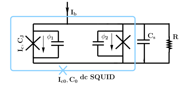
Figure 1: (Color-online) Flux qubit measured by a dc-SQUID gray (blue) line. The qubit corresponds to the inner SQUID loop with critical current $I_{c}$ and capacitance $C_{J}$ for both Josephson junctions denoted by the large $\times$ symbol. The inner SQUID is shunted by a capacitance $C_{s}$, and environmental resistance $R$ and is biased by a ramping current $I_{b}$. The dc-SQUID loop has junction capatitance $C_{0}$ and critical current $I_{c0}$.

In Fig. 1, we show a flux qubit (inner-loop), which is measured by a dc-SQUID (outer loop). To study the decoherence and relaxation time scales in such a system it is necessary to understand how noise is transferred from from the dc-SQUID to the qubit.

For the circuit displayed in Fig. 1, the classical equation of motion for the dc-SQUID (outer-loop) is

$$C_{0}\ddot{\phi}+\frac{2\pi}{\Phi_{0}}I_{c0}\sin\phi-\frac{2\pi}{\Phi_{0}}I+\int_{0}^{t}dt^{\prime}Y(t-t^{\prime})\dot{\phi}(t^{\prime})=0$$ (1)

where $\phi$ is the gauge invariant phase across the Josephson junction of the dc-SQUID, $I_{c0}$ is the critical current of its junction, $\Phi_{0}=h/2e$ is the flux quantum. The last term in Eq. (1) is the dissipation term due to effective admittance $Y(\omega)$ felt by the outer dc-SQUID. In this case the total induced current in the dc-SQUID (outer loop) is tian-02

$$I=\left(\frac{\Phi_{0}}{2\pi}\right)\frac{4}{L_{dc}}\langle\delta\phi_{0}\sigma_{z}\rangle+\left(\frac{\Phi_{0}}{2\pi}\right)\frac{4}{L_{dc}}\langle\phi_{m}\rangle+\left(\frac{2\pi}{\Phi_{0}}\right)J_{1}\langle\phi_{p}\rangle.$$ (2)

Here $\phi_{p}=(\phi_{1}+\phi_{2})$ and $\phi_{m}=(\phi_{2}-\phi_{1})$ are the sum and difference of the gauge invariant phases $\phi_{1}$ and $\phi_{2}$ across the junctions of the inner SQUID, $L_{dc}$ is the self-inductance of the inner SQUID, and $J_{1}$ is the bilinear coupling between $\phi_{m}$ and $\phi_{p}$ at the potential energy minimum. The term $\delta\phi_{0}=\pi M_{q}I_{cir}/\Phi_{0}$, where $I_{cir}$ is the circulating current of the localized states of the qubit (described in terms of Pauli matrix $\sigma_{z}$), and $M_{q}$ is the mutual inductance between the qubit and the outer dc-SQUID.

For the charge qubit coupled to a transmission line resonator blais-04 ; koch-07 shown in Fig. 2, the classical equation of motion for the charge Q is

$$V_{g}(\omega)=\left(-\frac{\omega^{2}L_{J}(\omega)}{1-\omega^{2}L_{J}(\omega)C_{J}}+\frac{1}{C_{g}}+i\omega Z(\omega)\right)Q(\omega)$$ (3)

Here, $V_{g}$ is the gate voltage, $C_{g}$ is the gate capacitance, $L_{J}$ and $C_{J}$ are the Josephson inductance and capacitance respectively, $Z(\omega)$ is the effective impedance seen by the charge qubit due to a transmission line resonator (cavity), and $Q$ is the charge across $C_{g}$.

Figure 2: Circuit diagram of the Cooper-pair box. The superconducting island (large $\times$) is connected to a large reservoir through a Josephson junction with Josephson energy $E_{J}$ and capacitance $C_{J}$. The voltage bias $V_{g}$ is provided through a resonator (cavity) having environmental impedance $Z(\omega)$, which is connected to the gate capacitance $C_{g}$ as shown.

In Fig. 3, we show the circuit for a phase qubit corresponding to an asymmetric dc-SQUID martinis-02 ; martinis-03 . The circuit elements inside the dashed box form an isolation network which serves two purposes: a) it prevents current noise from reaching the qubit junction; b) it is used as a measurement tool.

The classical equation of motion for the phase qubit shown in Fig. 3 is

$$C_{0}\ddot{\gamma}+\frac{2\pi}{\Phi_{0}}I_{c0}\sin\gamma-\frac{2\pi}{\Phi_{0}}I+\int_{0}^{t}dt^{\prime}Y(t-t^{\prime})\dot{\gamma}(t^{\prime})=0,$$ (4)

where $C_{0}$ is the capacitance, $I_{c0}$ is the critical current, and $\gamma$ is the phase difference across the Josephson junction $J$ (large $\times$ in Fig. 3), while $I$ is the bias current, and $\Phi_{0}=h/2e$ is the flux quantum. The last term of Eq. (4) can be written as $i\omega Y(\omega)\gamma(\omega)$ in Fourier space. The admittance function $Y(\omega)$ can be modeled as two additive terms $Y(\omega)=Y_{iso}(\omega)+Y_{int}(\omega)$. The first contribution $Y_{iso}(\omega)$ is the admittance that results when a transmission line of characteristic impedance $R$ is attached to the isolation junction (here represented by a capacitance $C$ and a Josephson inductance $L$) and an isolation inductance $L_{1}$. Thus, $Y_{iso}(\omega)=Z_{iso}^{-1}(\omega)$ where $Z_{iso}(\omega)=(i\omega L_{1})+\left[R^{-1}+i\omega C+(i\omega L)^{-1}\right]^{-1}$ is the impedance of the isolation network shown in Fig. 3. The replacement of the isolation junction by an LC circuit is justified because under standard operating conditions the external flux $\Phi_{\rm a}$ varies to cancel the current flowing through the isolation junction making it zero biased martinis-02 . Thus, the isolation junction behaves as a harmonic oscillator with inductance $L$ which is chosen to be much smaller than $L_{1}$. The second contribution $Y_{int}(\omega)$ is an internal admittance representing the local environment of the qubit junction, such as defects in the oxide barrier, quasiparticle tunneling, or the substrate, and can be modeled by $Y_{int}(\omega)=(R_{0}+i\omega L_{0})^{-1}$, where $R_{0}$ is the resistance and $L_{0}$ is the inductance of the qubit as shown in Fig. 3.

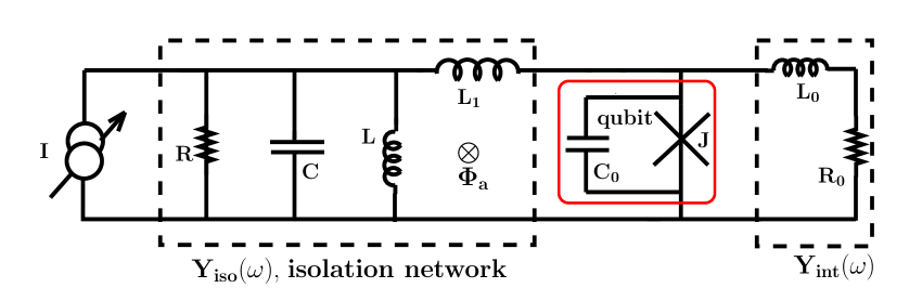
Figure 3: (Color-online) Schematic drawing of a phase qubit with an RLC isolation circuit. The phase qubit is shown inside the solid (red) box, the RLC isolation circuit is shown inside the dashed box to the left, and the internal admittance circuit is shown inside the dashed box to the right.

The equations of motion described in Eqs. (1), (3), and (4), can be all approximatelly described by the effective spin-boson Hamiltonian

$$\widetilde{H}=\frac{\hbar\omega_{01}}{2}\sigma_{z}+\sum_{k}\hbar\omega_{k}b_{k}^{\dagger}b_{k}+H_{SB},$$ (5)

written in terms of Pauli matrices $\sigma_{i}$ (with $i=x,y,z$) and boson operators $b_{k}$ and $b_{k}^{\dagger}$. The first term in Eq. (5) represents a two-level approximation for the qubit (system) described by states $|0\rangle$ and $|1\rangle$ with energy difference $\hbar\omega_{01}$. The second term corresponds to the isolation network (bath) represented by a bath of bosons, where $b_{k}$ and $b_{k}^{\dagger}$ are the annihilation and creation operator of the $k$-th bath mode with frequency $\omega_{k}$. The third term is the system-bath (SB) Hamiltonian which corresponds to the coupling between the environment and the qubit.

At the charge degeneracy point for the charge qubit (gate charge $N_{g}=0$), at the flux degeneracy point (external flux $\Phi_{\rm ext}=\pi\Phi_{0}$) for the flux qubit, and at the suitable flux bias condition for the phase qubit (external flux $\Phi_{\rm a}=L_{1}\phi_{0}$) $H_{SB}$ reduces to

$$H_{SB}=\frac{1}{2}\sigma_{x}\hbar\langle 1|v|0\rangle\sum_{k}\lambda_{k1}\left(b_{k}^{\dagger}+b_{k}\right)$$ (6)

where $v=\phi$ for the flux qubit, $v=Q$ for the charge qubit, and $v=\gamma$ for the phase qubit. The spectral density of the bath modes

$$J(\omega)=\hbar\sum_{k}\lambda_{k}^{2}\delta\left(\omega-\omega_{k}\right)$$ (7)

has dimensions of energy and can be written as

$$J(\omega)=\omega{\rm Re}Y(\omega)\left(\frac{\Phi_{0}}{2\pi}\right)^{2}$$ (8)

for flux and phase qubits or as

$$J(\omega)=2\hbar\omega{\rm Re}Z(\omega)\frac{e^{2}}{\hbar}$$ (9)

for charge qubits.

For the flux qubit circuit shown in Fig. 1, the shunt capacitance $C_{s}$ is used to control the environment, while the Ohmic resistance of the circuit is modelled by $R$. In this case, the environmental spectral density is tian-02

$$J_{1}\left(\omega\right)=\frac{\alpha_{1}\omega}{\left(1-\omega^{2}/\Omega_{1}^{2}\right)^{2}+4\omega^{2}\Gamma_{1}^{2}/\Omega_{1}^{4}}.$$ (10)

when $\omega_{m}\gg{\rm max}(\Omega_{1},\omega_{01})$, and when the dc-SQUID is far away from the switching point to be modelled by an ideal inductance $L_{J}$. The inner oscillator frequency $\omega_{m}=\sqrt{2/L_{dc}C_{J}}$ and the qubit frequency is $\omega_{01}$. The external oscillator frequency

$$\Omega_{1}=\sqrt{2\pi I_{c}^{\rm eff}/C_{s}\Phi_{0}}[1-(I_{b}/I_{c}^{\rm eff})^{2}]^{1/4},$$ (11)

and plays the role of the resonant frequency, where $I_{c}$ is the critical current for each of two Josephson junctions. Also, $\Gamma_{1}={1}/(C_{s}R)$ corresponds to the resonance width, and

$$\alpha_{1}=\frac{2(eI_{cir}I_{b}M_{q})^{2}}{C_{s}^{2}\hbar^{2}R\Omega_{1}^{4}}$$ (12)

reflects the low frequency behavior. The coupling between the flux qubit and the outer dc-SQUID emerges from the interaction of the persistent current $I_{cir}$ of the qubit and the bias current $I_{b}$ of the dc-SQUID via their mutual inductance $M_{q}$.

The spectral density for the charge qubit shown in Fig. 2 is obtained via Eq. (9) by determining the real part of the impedance $Z(\omega)$. In this case, we need to solve for the normal modes of the resonator and transmission lines, including an input impedance $R$ at each end of the resonator. This procedure results in the spectral density blais-04

$$J_{2}\left(\omega\right)=\frac{e^{2}\Omega_{2}}{\ell c}\frac{\Gamma_{2}}{(\omega-\Omega_{2})^{2}+(\Gamma_{2}/2)^{2}},$$ (13)

where $\Omega_{2}$ is the resonator frequency, $\ell$ is resonator length, $c$ is the capacitance per unit length of the transmission line. The quantity $\Gamma_{2}=\Omega_{2}/Q$ where $Q$ is the quality factor of the cavity.

For the phase qubit shown in Fig. 3, the spectral density $J(\omega)$ is given by Eq. (8), and can be written in the compact form $J(\omega)=J_{iso}(\omega)+J_{int}(\omega)$. The spectral density of the isolation network is

$$J_{iso}\left(\omega\right)=\left(\frac{\Phi_{0}}{2\pi}\right)^{2}\frac{\alpha\omega}{\left(1-\omega^{2}/\Omega^{2}\right)^{2}+4\omega^{2}\Gamma^{2}/\Omega^{4}},$$ (14)

where $\alpha=L^{2}/\left[(L+L_{1})^{2}R\right]\approx(L/L_{1})^{2}/R$ is the leading order term in the low frequency ohmic regime,

$$\Omega=\sqrt{\frac{(L+L_{1})}{LL_{1}C}}\approx\frac{1}{\sqrt{LC}}$$ (15)

is essentially the resonance frequency, and $\Gamma=1/(2CR)$ plays the role of resonance width. Here, we used $L_{1}\gg L$ corresponding to the relevant experimental regime. Notice that $J_{iso}(\omega)$ has Ohmic behavior at low frequencies since

$$\lim_{\omega\rightarrow 0}\frac{J_{iso}(\omega)}{\omega}=\left(\frac{\Phi_{0}}{2\pi}\right)^{2}\left(\frac{L}{L_{1}}\right)^{2}\frac{1}{R},$$ (16)

but has a peak at frequency $\Omega$ with broadening controlled by $\Gamma$. In addition, notice that the parameter

$$\frac{\Gamma}{\Omega^{2}}=\frac{LL_{1}}{\left(2R\left(L_{1}+L\right)\right)}\approx\frac{L}{R}$$ (17)

is independent of $C$. Therefore, when there is no capacitor ($C\to 0$), the resonance disappears and

$$J_{iso}(\omega)=\left(\frac{\Phi_{0}}{2\pi}\right)^{2}\frac{\alpha\omega}{1+4\omega^{2}\Gamma^{2}/\Omega^{4}},$$ (18)

reduces to a Drude term with characteristic frequency $\Omega^{2}/2\Gamma\approx R/L$. The internal spectral density of the qubit

$$J_{int}\left(\omega\right)=\left(\frac{\Phi_{0}}{2\pi}\right)^{2}\frac{(\omega/R_{0})}{1+\omega^{2}L_{0}^{2}/R_{0}^{2}}$$ (19)

is a Drude term with characteristic frequency $R_{0}/L_{0}$. Notice that $J_{int}(\omega)$ also has Ohmic behavior at low frequencies since

$$\lim_{\omega\rightarrow 0}\frac{J_{int}(\omega)}{\omega}=\left(\frac{\Phi_{0}}{2\pi}\right)^{2}\frac{1}{R_{0}}.$$ (20)

Having discussed the spectral functions of the environment of three different types of superconducting qubits and their corresponding circuits, we move next to the discussion of the decoherence properties within the Bloch-Redfield description of the time evolution of the density matrix.

III Bloch-Redfield equations: decoherence properties

In this section, we investigate the relaxation $T_{1}$ and decoherence $T_{2}$ times, for the three types of superconducting qubits (flux, charge and phase) described in section II. In order to obtain $T_{1}$ and $T_{2}$, we write the Bloch-Redfield equations weiss-99

$$\dot{\rho}_{nm}=-i\omega_{nm}\rho_{nm}+\sum_{kl}R_{nmkl}\rho_{kl}$$ (21)

for the density matrix $\rho_{nm}$ of the spin-boson Hamiltonian in Eq. (5) and (6) derived in the Born-Markov limit. Here all indices take the values $0$ and $1$ corresponding to the ground and excited states of the qubit, respectively, while $\omega_{nm}=(E_{n}-E_{m})/\hbar$ is the frequency difference between states $n$ and $m$. The Redfield rate tensor is

$$R_{nmkl}=-\Gamma_{lmnk}^{(1)}-\Gamma_{lmnk}^{(2)}+\delta_{nk}\Gamma_{lrrm}^{(1)}+\delta_{lm}\Gamma_{nrrk}^{(2)},$$ (22)

where repeated indices indicate summation, and

$$\Gamma_{lmnk}^{(1)}=\hbar^{-2}\int_{0}^{\infty}dte^{-i\omega_{nk}t}\langle H_{SB,lm}(t)H_{SB,nk}(0)\rangle,$$ (23)

$$\Gamma_{lmnk}^{(2)}=\hbar^{-2}\int_{0}^{\infty}dte^{-i\omega_{lm}t}\langle H_{SB,lm}(0)H_{SB,nk}(t)\rangle.$$ (24)

Under these conditions, the relaxation rate becomes

$$\frac{1}{T_{1}}=-\sum_{n}\limits R_{nnnn}=\frac{J(\omega_{01})}{M\omega_{01}}\coth\left(\frac{\hbar\omega_{01}}{k_{B}T}\right),$$ (25)

where we used the transition probability $|\langle 0|\nu|1\rangle|^{2}=\left[M\omega_{01}\right]^{-1}$ to define the variable $M$, which has dimensions of mass $\times$ area (or energy $\times$ squared-time) and is refered to as the mass of the qubit. For the flux and phase qubits, the mass is $M\equiv\left(\Phi_{0}/2\pi\right)^{2}C_{0}$, where $C_{0}$ is the capacitance of the qubit. For the charge qubit, the mass is $M\equiv\hbar e/I_{0}$, where $I_{0}$ is the critical current. The frequency $\omega_{01}$ is the qubit frequency.

The physical interpretation of $T_{1}^{-1}$ is as follows. For the system to make a transition it needs to exchange energy $E=\hbar\omega_{01}$ with the environment using a single boson. The factor $\coth(\hbar\omega_{01}/k_{B}T)=n(\omega_{01})+1+n(\omega_{01})$ captures the sum of the rates for emission (proportional to $n(\omega_{01})+1$) and absorption (proportional to $n(\omega_{01})$ of a boson), where $n(\omega_{01})=\left[\exp(\hbar\omega_{01}/k_{B}T)-1\right]^{-1}$ is the Bose function.

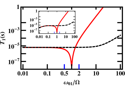
Figure 4: (Color-online) $T_{1}$ (in seconds) as a function of qubit frequency $\omega_{01}$. The solid (red) curves describe the phase qubit with RLC isolation network (Fig. 3) with parameters $R=50$ ohms, $L_{1}=3.9$nH, $L=2.25$pH, $C=2.22$pF, and qubit parameters $C_{0}=4.44$pF, $R_{0}=\infty$ and $L_{0}=0$. The dashed curves correspond to an RL isolation network with the same parameters, except that $C=0$. Main figure ($T=0$), inset ($T=50$mK) with $\Omega=141\times 10^{9}$ rad/sec.

Similarly, the decoherence rate given by the off-diagonal elements of the reduced density matrix $\rho$ is

$$\frac{1}{T_{2}}={\rm Re}(R_{nmnm})=\frac{1}{2T_{1}}+\frac{1}{T_{\phi}},$$ (26)

where the dephasing rate

$$\frac{1}{T_{\phi}} = |\langle 0|\nu|0\rangle-\langle 1|\nu|1\rangle|^{2}\mathop{\lim}\limits_{\omega\to 0}\frac{J(\omega)}{\omega}2k_{B}T$$ (27)

This contribution originates from dephasing processes which randomize the phases while keeping energy constant, i.e., transitions from a state into itself. Hence, they exchange zero energy with the environment and $J(0)$ enters. The prefactor measures which fraction of the total environmental noise leads to fluctuations of the energy splitting, such that only the components of noise which are diagonal in the basis of energy eigenstates leads to pure dephasing wilhelm-06 . This effect, is thus complementary to that of the off-diagonal transition matrix element $\langle 0|\nu|1\rangle$ which appears in $T_{1}$. The zero frequency argument is a consequence of the Markov approximation. Typically, $T_{\phi}\gg T_{1}$. This can be seen for example, in the Hamiltonian of the phase qubit, where $\langle 0|\gamma|0\rangle\sim\langle 1|\gamma|1\rangle\sim\partial^{3}U/\partial\gamma^{3}$ is the cubic correction to the potential of the phase qubit.

In Fig. 4, $T_{1}$ is plotted for the phase qubit as a function of the qubit frequency $\omega_{01}$ in the case of spectral densities describing an RLC [Eq. (14)] or Drude [Eq. (18)] isolation network at fixed temperatures $T=0$ (main figure) and $T=50$mK (inset), with $J_{int}(\omega)=0$ corresponding to $R_{0}\to\infty$. In the limit of low temperatures $(k_{B}T/\hbar\omega_{01}\ll 1)$, the relaxation time becomes

$$T_{1}(\omega_{01})=\frac{M\omega_{01}}{J(\omega_{01})}.$$ (28)

From the main plot of Fig. 4 several important points can be extracted. First, in the low frequency regime ($\omega_{01}\ll\Omega)$ the RL (Drude) and RLC environments produce essentially the same relaxation time $T_{1,RLC}(0)=T_{1,RL}(0)=T_{1,0}\approx(L_{1}/L)^{2}RC_{0}$, because both systems are ohmic. Second, near resonance ($\omega_{01}\approx\Omega$), $T_{1,RLC}$ is substantially reduced because the qubit is resonantly coupled to its environment producing a distinct non-ohmic behavior. Third, for ($\omega_{01}>\Omega$), $T_{1}$ grows very rapidly in the RLC case. Notice that for $\omega_{01}>\sqrt{2}\Omega$, the RLC relaxation time $T_{1,RLC}$ is always larger than $T_{1,RL}$. Furthermore, in the limit of $\omega_{01}\gg{\rm max}\{{\Omega,2\Gamma}\}$, $T_{1,RLC}$ grows with the fourth power of $\omega_{01}$ behaving as

$$T_{1,RLC}\approx T_{1,0}\frac{\omega_{01}^{4}}{\Omega^{4}},$$ (29)

while for $\omega_{01}\gg\Omega^{2}/2\Gamma$, $T_{1,RL}$ grows only with second power of $\omega_{01}$ behaving as

$$T_{1,RL}\approx 4T_{1,0}\frac{\Gamma^{2}\omega_{01}^{2}}{\Omega^{4}}.$$ (30)

Thus, $T_{1,RLC}$ is always much larger than $T_{1,RL}$ for sufficiently large $\omega_{01}$. For parameters in the experimental range (Fig. 4), $T_{1,RLC}$ is two orders of magnitude larger than $T_{1,RL}$, indicating a clear advantage of the RLC environment shown in Fig 1 over the standard ohmic RL environment. Thermal effects are shown in the inset of Fig. 4, where $T=50$mK is a characteristic experimental temperature paik-08 . Typical values of $T_{1}$ at low frequencies vary from $10^{-5}$s at $T=0$ to $10^{-6}$s at $T=50$mK, while the high frequency values remain essentially unchanged as thermal effects are not important for $\hbar\omega_{01}\gg k_{B}T$.

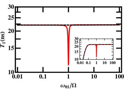
Figure 5: (Color-online) $T_{1}$ (in nanoseconds) as a function of qubit frequency $\omega_{01}$. The solid (red) curves describe a phase qubit with RLC isolation network (Fig. 3) with same parameters of Fig. 2 except that $R_{0}=5000$ ohms. The dashed curves correspond to an RL isolation network with the same parameters of the RLC network, except that $C=0$. Main figure ($T=0$), inset ($T=50$mK) with $\Omega=141\times 10^{9}$ rad/sec.

In the preceeding analysis we neglected the effect of the local environment by setting $Y_{int}(\omega)=0$. As a result, the low-frequency value of $T_{1}$ is substantially larger than obtained in experiment martinis-02 ; paik-08 . By modeling the local environment with $R_{0}=5000$ ohms and $L_{0}=0$, we obtain the $T_{1}$ versus $\omega_{01}$ plot shown in Fig. 5. Notice that this value of $R_{0}$ brings $T_{1}$ to values close to $20$ns at $T=0$. The message to extract from Figs. 4 and 5 is that increasing $R_{0}$ as much as possible and increasing the qubit frequency $\omega_{01}$ from $0.1\Omega$ to $2\Omega$ at fixed low temperature can produce a large increase in $T_{1}$.

Having discussed the decoherence properties caused by environments with resonances for the case of superconducting qubits, we discuss next how the environment shifts (renormalizes) the qubit frequency for the same systems.

IV Frequency renormalization

In this section, we discuss another effect of the environment on qubit properties, in addition to dephasing and relaxation. The environment also renormalizes (shifts) the qubit frequency $\omega_{01}$ by dressing the two-state system with environmental degrees of freedom. This is similar to the physics of the Lamb shift or the Franck Condon effect. In our case, the transition frequency $E=\omega_{01}$ is renormalized according to $E_{R}=E+\delta E$, where $\delta E=-{\rm Im}R_{1010}$ in terms of the Redfield rate tensor. The energy shift can be explicitly written as

$$\delta E=\frac{1}{4\pi}{\cal P}\int_{0}^{\infty}d\omega\frac{J(\omega)}{E^{2}-\omega^{2}}\left[E\coth(\beta\omega/2)-\omega\right],$$ (31)

where ${\cal P}$ denotes the Cauchy principal value, and $\beta=1/k_{B}T$. Notice that $\delta E$ is analogous to the energy shift obtained in second order perturbation theory, which collects all processes in which a virtual boson is emitted and reabsorbed, such that no trace is left in the environment. The integral in Eq. (31) can be calculated by extending the integration to the complete real axis, closing the countour in the upper complex plane, and applying the residue theorem.

IV.1 Phase and flux qubits

For phase and flux qubit discussed above, upon summation over all residues of the relevant poles of the spectral density, we arrive to wilhelm-03

$$\delta E=\frac{K}{2\pi}\frac{\Omega^{3}E}{2i\Gamma}\sum_{\sigma=\pm}\frac{\sigma}{E^{2}-(\sigma\Omega+i\Gamma)^{2}}\times$$

$$\left[G(\Gamma-i\sigma)-{\rm Re}G(iE)-\pi\frac{\Gamma-i\sigma\Omega}{E}\right]$$ (32)

where $G(x)=\psi(1+\beta x/2\pi)+\psi(\beta x/2\pi)$ involves the digamma function $\psi$, and $K=\alpha(\Phi_{0}/2\pi)^{2}$ for phase qubit [see Eq. (14)], and $K=\alpha_{1}$ [see Eq. (10)] for the flux qubit. Although, we use a compact notation involving complex functions, the energy correction $\delta E$ is real. Notice that $\delta E$ changes sign at $\omega\simeq E$, leading to an upward shift (renormalization) of $E$ if most of the spectral weight of $J(\omega)$ is above $E$ (corresponding to $E<\Omega$) whereas $E$ shifts downward in the opposite case. Physically, this corresponds to level repulsion between the spin and the oscillators in the environment. This result is consistent with usual second-order perturbation theory for energies. If the spectral weight $J(\omega)$ is concentrated at frequency $\omega=\Omega$, then the sign changes of $\delta E$ happens at $E\simeq\Omega$, leading to a rather sharp structure in $\delta E(\Omega)$, and in $E_{R}(\Omega)$.

In the limit of low temperatures $(T\to 0)$, we can replace the function $G$ appearing in Eq. (32) by an appropriate logarithm to find

$$\delta E=\frac{K}{2\pi}\frac{i\Omega^{3}E}{\Gamma}\sum_{\sigma=\pm}\frac{\sigma}{E^{2}-(\sigma\Omega+i\Gamma)^{2}}\log\left(\frac{\Gamma-i\sigma\widetilde{\Omega}}{iE}\right),$$ (33)

where $\widetilde{\Omega}=\Omega-\Gamma^{2}/\Omega$. In the underdamped limit $\Omega\gg\Gamma$, one approximates the logarithm by $\log|\Omega/E|-i\sigma\pi/2$ and rewrite the result as $E_{R}=E+\delta E$, with $\delta E=\delta E_{\Omega}+\delta E_{\rm res}$. The first term of $\delta E$ contains a logarithmic contribution which resembles the scaling in the Ohmic case (with cutoff frequency $\widetilde{\Omega}$),

$$\delta E_{\Omega}=\frac{2}{\pi}J(E)\log\left|\frac{E}{\widetilde{\Omega}}\right|.$$ (34)

where $\widetilde{\Omega}\approx\Omega$. This contribution changes sign from an upward shift at $E>\widetilde{\Omega}$ to a downward shift at $E<\widetilde{\Omega}$ as expected from the general arguments described above.

The other contribution to $\delta E$ takes into account the enormous spectral weight of the resonance, and can be written as

$$\delta E_{\rm res}=J(E)\frac{E^{2}-\widetilde{\Omega}^{2}}{\Omega\Gamma}.$$ (35)

A term of this kind persists even in the absence of damping of the external oscillator. This term vanishes linearly with $E$ at low energies, but undergoes the expected sign change near resonance $E\approx\Omega$, in which vicinity, a substantial renormalization also occurs.

As an illustration of the qualitative results discussed in this section, we show in Fig. 6 the frequency shift (renormalization) of the phase qubit with RLC isolation network described in Fig. 3. We make the identification $E=\omega_{01}$ and $\delta E=\delta\omega_{01}$. Near resonance $\omega_{01}\approx\Omega$, we find a frequency renormalization of about $2\%$ which is due to the term $\delta E_{res}$.

Figure 6: Renormalization of energy splitting for the phase qubit with RLC isolation network (Fig. 3) for the parameters $R=50$ ohms, $L_{1}=3.9$nH, $L=2.25$pH, $C=2.22$pF, and qubit parameters $C_{0}=4.44$pF, $R_{0}=5000$ ohms and $L_{0}=0$, $T=0$, and $\Omega=141\times 10^{9}$ rad/sec.

Next, we discuss briefly the frequency renormalization of charge qubits due to environmental effects.

IV.2 Charge qubits

For charge qubits with spectral density given by Eq. (13), the energy renormalization $\delta E$ obtained in Eq. (31) can be also calculated using complex integration techniques. In the low temperature limit $(T\to 0)$ there are two contributions to

$$\delta E=\delta E_{\Omega}+\delta E_{res}.$$ (36)

The first one is a resonant contribution

$$\delta E_{res}=e^{2}\frac{\Omega_{2}^{2}}{lc}\frac{\Lambda_{2}\left[\pi+2\arctan(2\Omega_{2}/\Gamma_{2})\right]}{\left(\Lambda_{2}^{2}+\Gamma_{2}^{2}\Omega_{2}^{2}\right)},$$ (37)

where the function

$$\Lambda_{2}=E^{2}-\Omega_{2}^{2}+\left(\frac{\Gamma_{2}}{2}\right)^{2}$$ (38)

and the second one is a non-resonant contribution

$$\delta E_{\Omega}=e^{2}\frac{\Omega_{2}^{2}}{lc}\frac{\Gamma_{2}\Omega_{2}\log\left[E^{2}/(\Gamma_{2}^{2}/4+\Omega_{2}^{2})\right]}{\left(\Lambda_{2}^{2}+\Gamma^{2}\Omega_{2}^{2}\right)}.$$ (39)

Just like the phase and flux qubit, the frequeny renormalization term due to the spectral weight of the resonance $\delta E_{res}$ is much larger than the logarithmic contribution $\delta E_{\Omega}$. While $\delta E_{res}$ undergoes a sign change from negative to positive at $E=\sqrt{\Omega_{2}^{2}-(\Gamma_{2}/2)^{2}}$, $\delta E_{\Omega}$ undergoes a sign change at $\sqrt{\Omega_{2}^{2}+(\Gamma_{2}/2)^{2}}$.

Having concluded the discussion of the frequency renormalization (shift) of superconducting qubits due to coupling to environments with resonant frequency $\Omega$, we discuss next the behavior of superconducting qubits coupled to the same environments, when the qubit frequency $\omega_{01}$ is close to $\Omega$, where essentially exact solutions are possible.

V Non-Markovian behavior near resonance

The Bloch-Redfield equations described in Eq. (21) capture the long time behavior of the density matrix, but can not describe the short time behavior of the system in particular near a resonance condition $\omega_{01}\approx\Omega$, where the environmental spectral density $J(\omega\approx\Omega)$ is very large. In this case, only the environmental modes with $\omega_{k}=\Omega$ couple strongly to the two-level system, like a two-level atom interacting with an electromagnetic field cavity mode that has a finite lifetime. Thus, next we derive the time evolution of the state of the flux, phase and charge qubits when the qubit frequency is close to an environmental resonance.

First, we restrict the Hamiltonian described in Eqs. (5) and (6) only to boson modes with $\omega_{k}\approx\Omega\approx\omega_{01}$. When $\omega_{k}\approx\Omega\approx\omega_{01}$, the Hamiltonian shown in Eqs. (5) and (6) can be solved in the rotating wave approximation using the complete basis set of system-bath product states $|\psi_{0}\rangle=|0\rangle_{\rm S}\otimes|0\rangle_{\rm B}$; $|\psi_{1}\rangle=|1\rangle_{\rm S}\otimes|0\rangle_{\rm B}$; $|\psi_{k}\rangle=|0\rangle_{\rm S}\otimes|k\rangle_{\rm B}$, where $|0\rangle_{\rm S}$ and $|1\rangle_{\rm S}$ are the states of the qubit and $|k\rangle_{\rm B}$ are the states of the bath. Notice that the states $|1\rangle_{\rm S}\otimes|k\rangle_{\rm B}$ are absent in the basis set within the rotating wave approximation and that the state of the total system at any time is

$$\phi(t)=c_{0}\psi_{0}+c_{1}(t)\psi_{1}+\sum_{k\neq 0,1}c_{k}(t)\psi_{k},$$ (40)

with probability amplitudes $c_{0}$, $c_{1}(t)$, and $c_{k}(t)$. The amplitude $c_{0}$ is constant, while the amplitudes $c_{1}(t)$ and $c_{k}(t)$ are time dependent. Assuming that there are no excited bath modes at $t=0$, we impose the initial condition $c_{k}(0)=0$, and use the normalization $|\phi(t)|^{2}=1$ to obtain the closed integro-differential equation

$$\dot{c}_{1}(t)=-\int_{0}^{t}dt_{1}f(t-t_{1})c_{1}(t_{1}),$$ (41)

where the kernel is the correlation function

$$f(\tau)=\int_{0}^{\infty}d\omega J(\omega)\exp\left[\text{i}(\omega_{01}-\omega)\tau\right]$$

directly related to the spectral density $J(\omega)$. The reduced density matrix

$$\rho(t)=\left(\begin{array}[]{cc}|c_{1}(t)|^{2}&c_{1}(t)c_{0}^{*}\\ c_{1}^{*}(t)c_{0}&|c_{0}|^{2}+\sum_{k}|c_{k}(t)|^{2}\end{array}\right)$$ (42)

is subject to the condition ${\rm Tr}\rho(t)=1$, or more explicitly $|c_{0}|^{2}+\sum_{k}|c_{k}(t)|^{2}=1-|c_{1}(t)|^{2}$, which shows that the time dynamics of $\rho(t)$ is fully determined by $c_{1}(t)$ for a specified value of $c_{0}$.

V.1 Phase and Flux qubits

For phase and flux qubita with spectral densities given by Eq. (14) and Eq. (10) respectively, we can rewrite the spectral density as

$$J_{\rm res}(\omega)=\frac{K\Omega^{3}}{4\text{i}\Gamma}\sum_{\sigma=\pm 1}\frac{\sigma\omega}{\omega^{2}-\left(\sigma\widetilde{\Omega}+\text{i}\Gamma\right)^{2}},$$ (43)

where $K=\alpha(\Phi_{0}/2\pi)^{2}$ for phase qubit [see Eq. (14], and $K=\alpha_{1}$ [see Eq. (10)] for the flux qubit. This reveals a resonance at $\omega=\widetilde{\Omega}$ with linewidth $\Gamma$, implying that any internal off-resonance contribution to $J(\omega)$, such as $J_{int}(\omega=\widetilde{\Omega})$ in the case of the phase qubit coupled to an RLC environment, can be neglected for any non-zero value of the resistance $R_{0}$. In this case, the spectral density $J(\omega)$ dominated by the resonant contribution $J(\omega)\approx J_{iso}(\omega)\approx J_{\rm res}(\omega)$. It is very important to emphasize, that eventhough $J_{\rm res}(\omega)$ is rewritten explicitly in terms of its poles in the complex plane, a simple inspection of Eq. (43) shows that $J_{\rm res}(\omega)$ is real.

For this spectral density, we can now solve for $c_{1}(t)$ exactly and obtain the closed form

$$c_{1}(t)={\cal L}^{-1}\left\{\frac{(s+\Gamma-i\omega_{01})^{2}+\Omega^{2}-\Gamma^{2}}{s\left[(s+\Gamma-i\omega_{01})^{2}+\Omega^{2}-\Gamma^{2}\right]-\kappa\Omega^{4}\pi i/\Gamma}\right\}$$

where ${\cal L}^{-1}\{F(s)\}$ is the inverse Laplace transform of $F(s)$, and $\kappa=K\times(\Phi_{0}/2\pi)^{2}\approx 1/(\omega_{01}T_{1,0})$.

In Fig. 7, we plot the density matrix element $\rho_{11}=|c_{1}(t)|^{2}$ as a function of time for the dc-SQUID phase qubit described in Fig 3. The plot contains curves for three different values of resistance, assuming that the qubit is initially (time $t=0$) in its excited state where $\rho_{11}(0)=1$. We consider the experimentally relevant weak dissipation limit of $\Gamma\ll\omega_{01}\approx\Omega$. Since $\Gamma=1/(2CR)$ the width of the resonance in the spectral density shown in Eq. (43) is smaller for larger values of $R$. Thus, for large $R$, the RLC environment transfers energy resonantly back and forth to the qubit and induces Rabi-oscillations with an effective time dependent decay rate $\gamma(t)=-2{\cal R}\{\dot{c}_{1}(t)/c_{1}(t)\}.$

These environmentally-induced Rabi oscillations are a clear signature of the non-Markovian behavior produced by the RLC environment, and are completely absent in the RL environment because the energy from the qubits is quickly dissipated without being temporarily stored. In the RL environment the decay in time of $\rho_{11}(t)$ has the characteristic non-oscillatory Markovian behavior. These environmentally-induced Rabi oscillations are generic features of circuits with resonances in the real part of the admittance. The frequency of the Rabi oscillations $\Omega_{Ra}=\sqrt{\pi\kappa\Omega^{3}/2\Gamma}$ is independent of the resistance since $\Omega_{Ra}\approx\Omega\sqrt{\pi L^{2}C/L_{1}^{2}C_{0}}$, and has the value of $\Omega_{Ra}=2\pi f_{Ra}\approx 360\times 10^{6}$ rad/sec in Fig. 7. This effect is similar to the so-called circuit quantum electrodynamics which has been of great experimental interest recently wallraff-04 ; chiorescu-04 ; sillanpaa-07

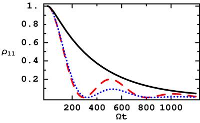
Figure 7: (Color-online) Population of the excited state of the dc-SQUID phase qubit (Fig. 3) as a function of time $\rho_{11}(t)$, with $\rho_{11}(t=0)=1$ for $R=50$ ohms (solid black curve), $350$ ohms (dotted blue curve), and $R=550$ ohms (dashed red curve), and $L_{1}=3.9$nH, $L=2.25$pH, $C=2.22$pF, $C_{0}=4.44$pF, $R_{0}=\infty$ and $L_{0}=0$.

Next, we discuss briefly the non-Markovian dynamics for charged qubits.

V.2 Charge qubits

For charge qubits, the spectral density in Eq. (13) can be rewritten in terms of its poles in the complex plane as

$$J(\omega)=\frac{e^{2}\Omega_{2}}{ilc}\sum_{\sigma=\pm 1}\frac{\sigma}{\omega-\Omega_{2}+\sigma i\Gamma_{2}/2}.$$ (44)

Again, we can solve for $c_{1}(t)$ exactly, which is now given by

$$c_{1}(t)=c_{1}(0)e^{-\Gamma_{2}t/4}\left(\cosh\frac{\Delta t}{2}+\frac{\Gamma_{2}}{2\Delta}\sinh\frac{\Delta t}{2}\right)$$ (45)

where $\Delta=\sqrt{\Gamma_{2}^{2}/4-8\pi e^{2}\Omega_{2}/lc}$. Notice that the frequency $\Delta$ can be complex, so it is convenient to rewrite it as

$$\Delta=\frac{\Gamma_{2}}{2}\sqrt{1-\left(\frac{2\Omega_{c}}{\Gamma_{2}}\right)\left(\frac{2\Omega_{2}}{\Gamma_{2}}\right),}$$ (46)

where $\Omega_{c}=8\pi e^{2}/\ell c$. In the underdamped case where $\Omega_{2}\gg\Gamma_{2}/2$, provided that $2\Omega_{c}/\Gamma_{2}$ is not too small, $\Delta$ becomes purely imaginary:

$$\Delta\approx i\sqrt{\Omega_{c}\Omega_{2}}.$$ (47)

Since $\cosh(i\theta)=\cos(\theta)$ and $\sinh(i\theta)=i\sin(\theta)$, where $\theta=(\sqrt{\Omega_{c}\Omega_{2}})t/2$ in the present case, it becomes clear that an oscillatory decay of the state emerges in the underdamped regime. In this regime, the period of oscillation is just $\tau=4\pi/\sqrt{\Omega_{c}\Omega_{2}}$.

Having completed our discussion of environmentally-induced Rabi oscillations and its markedly non-markovian characteristic, we are ready to conclude.

VI Conclusions

In conclusion, we analyzed decoherence effects in qubits coupled to environments containing resonances in their spectral function, and we identified a crucial role played by the design of isolation circuits on decoherence properties. Furthermore, we found that the decoherence time of qubits can be two orders of magnitude larger than their typical low-frequency ohmic-regime, provided that the frequency of the qubit is about two times larger than the resonance frequency of the environmental resonance (isolation circuit in the phase qubit case). We also studied the frequency renormalization (shift) of the qubit described by a two-level system due to dressing of the energy levels by the environmental degrees of freedom. We found that the frequency shift changes sign across the resonance frequency and is largest at resonance (about $2\%$). Lastly, we showed that when the qubit frequency is close to a resonance of the environment, the non-oscillatory Markovian decay of the excited state population of the qubit, gives in to an oscillatory non-Markovian decay, as the qubit and its environment self-generate Rabi oscillations of characteristic time scales shorter than the decoherence time. In particular, we discussed as a concrete example the decoherence properties of a dc-SQUID phase qubit coupled with an environmental RLC circuit possesing a resonance in its spectral function, where numbers compatible with current experiments were used to estimate the environmental effects on decoherence properties mitra-08 ; paik-08 .

- (1) C. Monroe, D. M. Meekhof, B. E. King, W. M. Itano, and D. J. Wineland, Phys. Rev. Lett. 75, 4714 (1995).
- (2) G. K. Brennen, C. M. Caves, P. S. Jessen, and I. H. Deutsch, Phys. Rev. Lett 82, 1060 (1999).
- (3) R. Hanson, B. Witkamp, L. M. K. Vandersypen, L. H. Willems van Beveren, J. M. Elzerman, and L. P. Kouwenhoven, Phys. Rev. Lett 91, 196802 (2003).
- (4) T. Hayashi, T. Fujisawa, H. D. Cheong, Y. H. Jeong, and Y. Hirayama, Phys. Rev. Lett 91, 226804 (2003).
- (5) D. Vion, A. Aassime, A. Cottet, P. Joyez, H. Pothier, C. Urbina, D. Esteve, M. H. Devoret, Science 296, 886 (2002).
- (6) R. C. Ramos et al., IEEE Trans. Appl. Supercond. 11, 998 (2001).
- (7) A. Shnirman, G. Schon, and Z. Hermon, Phys. Rev. Lett 79, 2371 (1997).
- (8) J. Martinis et al., Phys. Rev. Lett. 95, 210503 (2005).
- (9) Kaushik Mitra, C. J. Lobb, and C. A. R. Sá de Melo, Phys. Rev. B 79, 132507 (2009).
- (10) J. E. Mooij, T. P. Orlando, L. Levitov, Lin Tian, Caspar H. van der Wal, Seth Lloyd, Science 285, 1036 (1999).
- (11) C. H. van der wal, F. K. Wilhelm, C. J. P. M. Harmans, J. E. Mooij, Eur. Phys. J. B 31, 111 (2003).
- (12) J. M. Martinis, S. Nam, J. Aumentado, and C. Urbina, Phys. Rev. Lett. 89, 117901 (2002).
- (13) J. Koch, T. M. Yu, J. Gambetta, A. A. Houck, D. I. Schuster, J. Majer, A. Blais, M. H. Devoret, S. M. Girvin, and R. J. Schoelkopf, Phys. Rev. A 76, 042319 (2007).
- (14) Lin Tian, Seth Lloyd, and T.P. Orlando, Phys. Rev. B 65, 144516 (2002).
- (15) Alexandre Blais, Ren-Shou Huang, Andreas Wallraff, S. M. Girvin, R. J. Schoelkopf, Phys. Rev. A 69, 062320 (2004).
- (16) J. M. Martinis, S. Nam, J. Aumentado, K. M. Lang, and C. Urbina, Phys. Rev. B 67, 094510 (2003).
- (17) A. J. Leggett, S. Chakravarty, A. T. Dorsey, Matthew P. A. Fisher, Anupam Garg, and W. Zwerger, Rev. Mod. Phys. 59, 1 (1987).
- (18) F. K. Wilhelm, M. J. Storcz, U. Hartmann, and M. R. Geller, NATO-ASI proceedings: Mathematics, Physics and Chemistry 244, 195 (2007)
- (19) U. Weiss, Quantum Dissipative Systems, World Scientific (1999).
- (20) F. K. Wilhelm, S. Kleff, and J. von Delft, Chemical Physics 296, 345, (2003)
- (21) Hanhee Paik, S. K. Dutta, R. M. Lewis, T. A. Palomaki, B. K. Cooper, R. C. Ramos, H. Xu, A. J. Dragt, J. R. Anderson, C. J. Lobb, and F. C. Wellstood, Phys. Rev. B 77, 214510 (2008).
- (22) A. Wallraff, D. I. Schuster, A. Blais, L. Frunzio, R.-S. Huang, J. Majer, S. Kumar, S. M. Girvin and R. J. Schoelkopf, Nature 431, 462 (2004).
- (23) I. Chioorescu, P. Bertet, K. Semba, Y. Nakamura, C. J. P. M. Harmans, and J. E. Mooij, Nature 431, 159 (2004).
- (24) Mike A. Sillanp , Jae I. Park, and Raymond W. Simmonds, Nature 449, 438 (2007).
- (25) Kaushik Mitra, F. W. Strauch, C. J. Lobb, J. R. Anderson, F. C. Wellstood, and Eite Tiesinga, Phys. Rev. B 77, 214512(2008).