Spatiotemporal chaos and the dynamics of coupled Langmuir and ion-acoustic waves in plasmas

Abstract

A simulation study is performed to investigate the dynamics of coupled Langmuir waves (LWs) and ion-acoustic waves (IAWs) in an unmagnetized plasma. The effects of dispersion due to charge separation and the density nonlinearity associated with the IAWs, are considered to modify the properties of Langmuir solitons, as well as to model the dynamics of relatively large amplitude wave envelopes.  It is found that the Langmuir wave electric field, indeed, increases by the effect of  ion-wave nonlinearity (IWN). Use of a low-dimensional model, based on three Fourier modes shows that a transition to temporal chaos is possible, when the length scale of the linearly excited modes is larger than that of the most unstable ones. The chaotic behaviors of the unstable modes are identified by the analysis of Lyapunov exponent spectra. The space-time evolution of the coupled LWs and IAWs shows that the IWN can cause the excitation of many unstable harmonic modes, and can lead to strong IAW emission. This occurs when the initial wave field is relatively large or the length scale of IAWs is larger than the soliton characteristic size. Numerical simulation also reveals that many solitary patterns can be excited and generated through the modulational instability (MI) of unstable harmonic modes.  As time goes on, these solitons are seen to appear in the spatially partial coherence (SPC) state due to the free ion-acoustic radiation as well as in the state of spatiotemporal chaos (STC) due to collision and fusion in the stochastic motion. The latter results the redistribution of initial wave energy into a few modes with small length scales, which may lead to the onset of Langmuir turbulence in laboratory as well as space plasmas.

LABEL:FirstPage1 LABEL:LastPage#1102

I Introduction

The formation of envelope solitons, through the nonlinear interaction of high-frequency (hf) electric fields and low-frequency (lf) ion-acoustic waves (IAWs) is one of the most interesting features, and is extensively studied problem in the context of turbulence in modern plasma physics. Formation of these structures not only plays a role in turbulence, but also for plasma heating, particle transport etc., and so their properties are of fundamental interest. In plasmas, such envelope solitons are well-known Langmuir solitons that are hf Langmuir waves (LWs) trapped by the density troughs associated with lf IAWs (see e.g., Refs. Zakharov ; Karpman1 ; Karpman2 ; Deeskow ; Schamel1 ; Schamel2 ).

During the past few years several attempts have been made to investigate the dynamics of solitons including dressed solitons Karpman2 , soliton collapse Hadzievski , nucleation of cavitons Doolen , radiation of Langmuir solitons Karpman1 , Landau damping in partially incoherent LWs Fedele etc. An experimental observation for the excitation of IAWs has also been reported in a Langmuir turbulence regime by Prado et al Prado . Moreover, an increasing interest has also been found to study the Langmuir turbulence as a result of chaos Misra1 ; Misra2 ; Misra3 ; Chain ; Batra ; Rizzato .   When the electric field intensity is strong enough to reach the modified decay instability threshold, the interaction between LWs and IAWs results to ‘weak turbulence’, and then the LWs are scattered off IAWs under $T_{e}>>T_{i},$ where $T_{(e,i)}$ is the electron (ion) temperature. On the other hand, when the field intensity is so strong that the modulational instability (MI) threshold is exceeded, the LWs are then essentially trapped by the density cavities associated with IAWs. Such phenomenon can occur frequently in plasmas. The interaction is then said to be in a ‘strong turbulence’ regime, in which transfer or redistribution of energy to higher harmonic modes with small wavelengths may be possible. In general, it is believed that some sort of chaotic process may be responsible for the energy transfer from large to small spatial scales Pettini ; Tsaur . This energy transfer may become faster when the chaotic process is well developed in a subsystem of the full set of equations Rizzato .

One of the most important models in this context is the so-called Zakharov equations (ZEs) Zakharov , which have been derived by assuming a quasineutrality as well as neglecting the ion-wave nonlinearity (IWN) due to density fluctuation. However, the effects of dispersion due to charge separation (deviation from the quasineutrality) may be important in the radiation of IAWs, i.e., when the LWs  resonantly interact with IAWs at the same speed Karpman1 ; Karpman2 .  On the other hand, when wave amplitude becomes relatively large, the IWN can be important in the enhancement of ion-acoustic wave emission as well as in the excitation of many unstable harmonic modes at the initial stage of interaction, which later turns out to spatiotemporal chaos (STC).

The basic purpose of this work is to investigate numerically the dynamics of coupled LWs and IAWs in presence of these important effects, and also to modify the results of Langmuir solitons not observed in the one-dimensional (1D) ZEs. We show that transfer of energy to fewer modes, indeed, occurs and it is faster when the chaotic process in a low-dimensional model of the full system is well developed by the IWN. Such low-dimensional model is constructed on the basis of three unstable harmonic modes Misra3 , and which depends on a particular regime of the wave number of excitation. Numerical simulation of this low-dimensional model reveals that transition from order to chaos is possible, when the largest length scale of the IAWs is greater than that of the soliton characteristic size. Solitons will then much be distorted by the IAW emission until a mostly chaotic state emerges. For details of the idea of constructing such model, readers are referred to the work in Ref. Rizzato .

Since the low-dimensional model is restricted to a few number of modes, and also it is valid for a certain vale of the wave number of excitation, one needs to investigate, e.g., numerically the the full space-time problem, especially when this wave number is small enough to excite many unstable modes. We show that these solitary patterns, thus formed, ultimate lose their strengths after a long time through the random collision and fusion under the strong IAW emission. The STC state of the system is then said to emerge. However, the mechanism leading to such STC is still not clear. A few works in this direction can be found in the literature Misra2 ; Rizzato ; He .

The paper is organized as follows. In Sec. II, we present the governing equations, and analyze the evolution of Langmuir solitons in some particular cases of interest. A low-dimensional three-wave model is formed and its linear stability analysis is carried out in Sec. III. Numerical results for the temporal evolution of the low-dimensional model and the spatiotemporal evolution of the full system are presented in Sec. IV and Sec. V respectively. Finally, Sec. VI contains some discussion and conclusion.

II Governing equations and the Langmuir soliton

The nonlinear interaction of hf LWs and lf IAWs is governed by the following coupled set of equations Karpman1 ; Karpman2

$$i\epsilon\frac{\partial E}{\partial t}+\frac{3}{2}\frac{\partial^{2}E}{\partial x^{2}} =\frac{\nu}{2}E,$$ (1)

$$\frac{\partial^{2}\nu}{\partial t^{2}}-\frac{\partial^{2}\nu}{\partial x^{2}}-\frac{\partial^{4}\nu}{\partial x^{2}\partial t^{2}} =\frac{\partial^{2}|E|^{2}}{\partial x^{2}}$$

$$+\frac{\partial^{4}|E|^{2}}{\partial x^{2}\partial t^{2}}-\frac{1}{2}\frac{\partial^{2}\nu^{2}}{\partial x^{2}}-\frac{1}{2}\frac{\partial^{4}\nu^{2}}{\partial x^{2}\partial t^{2}},$$ (2)

where $E(x,t)$ is the slowly varying Langmuir wave electric field normalized by $\sqrt{16\pi n_{0}k_{B}T_{e}},$ with $n_{0}$ denoting the equilibrium number density, $k_{B}$ is the Boltzmann constant, $\epsilon\equiv\sqrt{m_{e}/m_{i}}$ is the square root of the electron-ion mass ratio and $\nu(x,t)\equiv n_{e1}/n_{0}=n_{e}-1$ is the plasma relative density fluctuation. The time $\ t$ is normalized by the ion plasma period $\omega_{pi}^{-1}\equiv 1/\sqrt{4\pi n_{0}e^{2}/m_{i}}$ and the space $x$ by the electron Debye radius $\lambda_{De}\equiv\sqrt{k_{B}T_{e}/4\pi n_{0}e^{2}}.$ In Eq. (2) the terms with fourth-order mixed derivatives describe the effects due to charge separation (i.e., deviation from the quasineutrality). The third and fourth terms in the right-hand side of Eq. (2) arise due to the expansion of $\log(1+\nu)$ up to the second order of $\nu$ in the equation for lf perturbation of electrons. This enforces us to assume that the relative density fluctuation associated with IAWs is not so small.

We note that the analytic treatment of the Eqs. (1) and (2) without IWN has been studied in detail for the modification of Langmuir solitons by Karpman et al Karpman1 ; Karpman2 . However, when the IWN is included in the system, the soliton properties may be changed.  To look for this effect, we simply disregard the mixed derivatives, and solve numerically the system of Eqs. (1) and (2) by Runge-Kutta scheme. In the scheme, we approximate the spatial derivatives by the centered second-order difference formulas, and use $\nu=E=\partial^{2}E/\partial x^{2}=\partial^{2}\nu/\partial x^{2}=0$ at the boundaries. The results are presented in Fig.1. When the ion-acoustic radiation is weak, we see that around $x=0$ the ponderomotive force dominates over the IWN, giving rise an increased amplitude of the envelope (highly correlated with the density depletion). However, in the other regimes of $x$, IWN dominates and makes the solitons wider. Later, we will see that as time progresses, the IAW emission increases by the IWN, causing solitons to lose their strengths.

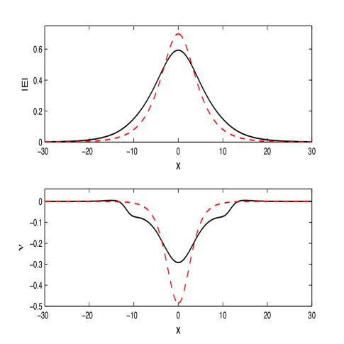
Figure 1: (Color online) The profiles of the Langmuir wave electric field (upper panel) and the associated density depletion (lower panel) are shown [solution of Eqs. (1) and (2)]. The solid and dashed (red) lines respectively correspond to the case with IWN and without IWN after $t=10(\omega_{pi}^{-1})$.

Some particular cases can be of interest in the context of Langmuir solitons. For example, under the small amplitude condition, i.e., disregarding the third  and fourth terms in the right-hand side of Eq. (2), and assuming the quasineutrality (disregarding the mixed fourth order derivatives), the dynamics of small amplitude IAWs are then governed by

$$\frac{\partial^{2}\nu}{\partial t^{2}}-\frac{\partial^{2}\nu}{\partial x^{2}}=\frac{\partial^{2}|E|^{2}}{\partial x^{2}}.$$ (3)

This equation when coupled with Eq. (1) describes under suitable renormalizations the classical ZEs Zakharov , which has been extensively studied in the context of Langmuir wave turbulence (see e.g., Hadzievski ; Doolen ; Prado ; Misra2 ; Misra3 ; Chain ).

Again, assuming a slow space-time response to the perturbations as $x\rightarrow\epsilon^{1/2}(x-t),t\rightarrow\epsilon^{3/2}t,$ i.e., ion perturbations move with the ion-acoustic speed, $c_{s}\equiv\sqrt{k_{B}T_{e}/m_{i}}$, and asuming the dependent variables to vary$\sim\epsilon,$ the IAWs can be described by the following modified Korteweg-de Vries (mKdV) equation Makhankov ; Nishikawa ; Ikezi

$$2\frac{\partial\nu}{\partial t}-\frac{1}{2}\frac{\partial\nu^{2}}{\partial x}+\frac{\partial^{3}\nu}{\partial x^{3}}+\frac{\partial|E|^{2}}{\partial x}=0.$$ (4)

The equation (1) together with Eq. (4) describe the dynamics of slowly varying Langmuir wave electric field coupled to the slow response of the density perturbations. These coupled equations predict a class of solutions with a bell-shaped Langmuir wave electric field profile arrested into the density cavity Nishikawa ; Ikezi .

We now turn out to the global behaviors of the system. To this end, we first renormalize the original variables (similar to the ZEs) as $x\rightarrow\epsilon x,t\rightarrow\epsilon t,\nu\rightarrow\nu/\epsilon^{2},E\rightarrow E/\epsilon,$ and obtain the condition for MI as given below. Thus, Eqs. (1) and (2) reduce to

$$2i\frac{\partial E}{\partial t}+3\frac{\partial^{2}E}{\partial x^{2}} =\nu E$$ (5)

$$\frac{\partial^{2}\nu}{\partial t^{2}}-\frac{\partial^{2}\nu}{\partial x^{2}}-\epsilon^{2}\frac{\partial^{4}\nu}{\partial x^{2}\partial t^{2}} =\frac{\partial^{2}|E|^{2}}{\partial x^{2}}$$

$$+\epsilon^{2}\frac{\partial^{4}|E|^{2}}{\partial x^{2}\partial t^{2}}-\frac{\epsilon^{2}}{2}\frac{\partial^{2}\nu^{2}}{\partial x^{2}}-\frac{\epsilon^{4}}{2}\frac{\partial^{4}\nu^{2}}{\partial x^{2}\partial t^{2}}$$ (6)

Clearly, the term proportional to $\epsilon^{4}(\sim 10^{-7})$ becomes smaller and can be neglected. However, the terms proportional to $\epsilon^{2}$ can no longer be neglected when the soliton attenuation becomes relatively larger.

Next, the linear stability analysis of the perturbations $\propto$ $\exp(ikx-i\omega t)$ [where $k$ $(\omega)$ is the wave number (frequency) of modulation] for Eqs. (5) and (6) gives the following growth rate of MI.

$$\gamma=\frac{k}{\sqrt{2\alpha}}\left[\sqrt{\Lambda^{2}+6\alpha\left(|E_{0}|^{2}-\frac{3k^{2}}{2}\right)}-\Lambda\right]^{1/2},$$ (7)

where $\alpha=1+k^{2}\epsilon^{2},$ $\Lambda=1+3k^{2}\left(3\alpha/2-\epsilon^{2}|E_{0}|^{2}\right)/2,$ and the MI sets in for $k$ satisfying $0<k<k_{c}\equiv\sqrt{2/3}|E_{0}|.$

III Low-dimensional (three-wave) model

We note that the system of Eqs. (5) and (6) is, in general, multi-dimensional. However, there may be the situation in which a few number of modes is more active than the remaining modes. Such cases are quite typical not only for Langmuir wave turbulence, but are rather general for parametric instabilities of hf waves interacting with lf ones close to the instability threshold.  In this way, Galerkin expansions and truncations to a few normal modes are commonly used to describe the basic features of the full dynamics by a low-dimensional model. However, we will see that the specific details of such model are highly dependent on the range for the basic wave number of modulation $k$. So, considering the dynamics of few coupled waves, we expand the envelope $E(x,t)$ and the density $\nu(x,t)$ as Rizzato

$$E(x,t) =\sum_{m=-M/2}^{+M/2}E_{m}(t)e^{imkx}=\sum_{m=-M/2}^{+M/2}\rho_{m}(t)e^{i\theta_{m}(t)}e^{imkx},$$ (8)

$$\nu(x,t) =\sum_{m=-M/2}^{+M/2}n_{m}(t)e^{imkx},$$ (9)

where $M=[k^{-1}]$ represents the number of modes, $\rho_{m}=\rho_{-m},\theta_{m}=\theta_{-m},n_{m}=n_{-m}$. Since in our case, $M=2,$ $\rho_{1}=\rho_{\pm 1},n_{1}=n_{\pm 1}$ etc., we can express the fields as (see for details Misra1 ; Misra3 ; Batra )

$$E =E_{0}+E_{1}\cos(kx)\equiv\sqrt{N}\sin\left(\frac{a}{2}\right)\exp(i\theta_{0})$$

$$+\sqrt{2N}\cos\left(\frac{a}{2}\right)\exp(i\theta_{1})\cos(kx)\,,$$ (10)

$$\nu =N+n_{1}\cos(kx)\,,$$ (11)

where $N$ $(\equiv n_{0})=|E_{-1}|^{2}+|E_{0}|^{2}+|E_{1}|^{2}$ is the conserved plasmon number. Also, $a,$ $\theta_{0},$ $\theta_{1}$ and $n_{1}$ are each a function of time $t$.  Inserting Eqs. (10) and (11) into the Eqs. (5) and (6), and following, e.g., Refs. Misra1 ; Misra3 ; Batra we obtain the following temporal system

$$\dot{a}=-\frac{n_{1}}{\sqrt{2}}\sin\varphi,$$ (12)

$$\dot{\varphi}=\frac{1}{2}\left(3k^{2}-\sqrt{2}n_{1}\cos\varphi\cot a\right)\,,$$ (13)

$$\ddot{n}_{1}=U_{1}n_{1}^{2}+U_{2}n_{1}+U_{3}\,,$$ (14)

where the ‘dot’ represents differentiation with respect to $t,$ $\varphi=\theta_{0}-\theta_{1},$ and $U_{1},$ $U_{2}$ and $U_{3}$ are given by

$$U_{1}(a,\varphi) =C_{1}\frac{\cos\varphi}{\sin a}\left(\sin^{2}\varphi+\cos^{2}a\right),$$

$$U_{2}(a,\varphi) =C_{2}+\left(C_{3}-U_{1}\sin a\right)\cos a,$$

$$U_{3}(a,\varphi) =C_{4}\sin a\cos\varphi.$$ (15)

Here the constants $C_{1},...,C_{4}$ are

$$C_{1} =\frac{Nk^{2}\epsilon^{2}}{\sqrt{2}(1+k^{2}\epsilon^{2})},C_{2}=-\frac{k^{2}\left(1-N\right)}{1+k^{2}\epsilon^{2}},$$

$$C_{3} =-\frac{3k^{2}}{\sqrt{2}}C_{1},C_{4}=\frac{\sqrt{2}Nk^{2}}{1+k^{2}\epsilon^{2}}\left(\frac{9k^{4}\epsilon^{2}}{4}-1\right)$$ (16)

The system of Eqs. (12)-(14)  can be recast as a set of four ordinary differential equations (ODEs):

$$\dot{x}_{1} =-\frac{1}{\sqrt{2}\epsilon}\,x_{3}\sin x_{2}\,,$$ (17)

$$\dot{x}_{2} =\frac{1}{2\epsilon}\left(3k^{2}-\sqrt{2}x_{3}\,\cos x_{2}\,\cot x_{1}\right)\,,$$ (18)

$$\dot{x}_{3} =x_{4}\,,$$ (19)

$$\dot{x}_{4} =U_{1}x_{3}^{2}+U_{2}x_{3}+U_{3}\,,$$ (20)

where $U_{1},U_{2},U_{3}$ are now functions of $x_{1},$ $x_{2},$ and we redefine the variables as $a=x_{1},\varphi=x_{2},n_{1}=x_{3},\dot{n}_{1}=x_{4}.$ The basic properties of the system can now be in order. It can be shown that the adiabatic limit of Eqs. (17)-(20) gives an integrable system, and hence nonchaotic Misra3 ; Batra ; Rizzato . Next, the local stability of the system about the fixed points $(x_{10},x_{20},x_{30},0)$ given by

$$\sin x_{20}=0,\cot x_{10}=\pm\frac{3k^{2}}{\sqrt{2}x_{30}},$$ (21)

$$\pm 3C_{3}k^{2}\pm\sqrt{2}C_{4}+C_{2}\sqrt{9k^{4}+2x_{30}^{2}}$$

$$+\frac{9C_{1}k^{4}}{\sqrt{2}}\left(\pm 1-\frac{3\sqrt{2}k^{2}}{9k^{4}+2x_{30}^{2}}\right)=0,$$ (22)

where $x_{30}\neq 0,\cos x_{20}=\pm 1,$ can be examined by linearizing the Eqs. (17)-(20), and solving the corresponding eigenvalue problem. The linearized set of equations in a neighborhood of $Q\equiv(x_{10},x_{20},x_{30},0)$ is

$$\dot{X}=Df(Q)X,$$ (23)

where $X$ $=[x_{1},x_{2},x_{3},x_{4}]$ is a column vector and $Df(Q)$ is the Jacobian matrix at $Q$, i.e.,

$$Df(Q)=\left(\begin{array}[c]{cccc}0&-p_{0}&0&0\\ q_{0}&0&-r_{0}&0\\ 0&0&0&1\\ A_{1}&A_{2}&A_{3}&0\end{array}\right),$$ (24)

The eigenvalue equation $|Df(Q)-\lambda I|=0$ then reads

$$\lambda^{4}+\left(A_{3}+p_{0}q_{0}\right)\lambda^{2}+\left(A_{2}r_{0}\right)\lambda$$

$$+p_{0}\left(A_{3}q_{0}-A_{1}r_{0}\right)=0,$$ (25)

where

$$p_{0}=\pm\frac{x_{30}}{\sqrt{2}\epsilon},q_{0}=\frac{p_{0}}{\sin^{2}x_{10}},r_{0}=\pm\frac{\cot x_{10}}{\sqrt{2}\epsilon},$$ (26)

$$A_{1} =-C_{3}\sin x_{10}\pm C_{4}\cos x_{10}$$

$$\pm C_{1}\cos^{2}x_{10}\left(1-\cos x_{10}\cot x_{10}\right)$$

$$\pm\left(C_{1}\cos x_{10}-\frac{x_{30}}{\sin x_{10}}\right)$$

$$\times\left(\sin(2x_{10})+\cot x_{10}\cos^{2}x_{10}\right),$$ (27)

$$A_{2}=\pm 2x_{30}\cos x_{10},A_{3}=A_{2}\cot x_{10}.$$ (28)

We numerically examine a set of fixed points satisfying Eqs. (21) and (22), and the linear stability of the system by the Routh-Hurwitz (RH) criteria. To this end, we use Carden’s method to look for a real solution of Eq. (22) when expressed it as a cubic in $\alpha\equiv\sqrt{2x_{30}^{2}+9k^{4}\text{ }}$. The range of $k$ and $N$ for such real $\alpha,$ and hence for $x_{30}$ are $0<k\leq 0.5<\sqrt{2/3}|E_{0}|$ and $0.6\leq N\leq 8.$ Thus, for a given set of values of $k$ and $N$, one can obtain a set of fixed points from Eqs. (21) and (22). Having obtained a set of fixed points, one can then numerically examine the coefficients of the depressed quartic [Eq. (25)] for $0<k\leq 0.5$ and $0.6\leq N\leq 8$. We find that in these regimes, coefficients of $\lambda^{2}$ and $\lambda$ are always positive, and the constant term changes sign as in Fig. 2. Here the shaded (white) region indicates the positive (negative) values of the constant term. The constant term is also positive for $0<k<0.49$ and $0.6\leq N\leq 8.$ Thus, by the RH criteria Eq. (25) has at least one root with positive real part when the constant term of the quartic is negative. The system of Eqs. (17)-(20) is then said to be linearly unstable.  As an illustration, the eigenvalues for $N=8$, $0.498\leq k\leq 0.5,$ are a pair of complex conjugates, one real positive $(>1)$ and one negative real roots.

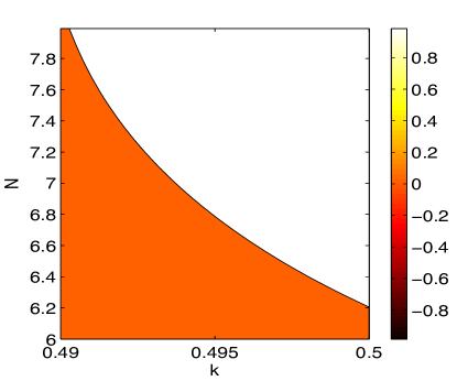
Figure 2: (Color online) The plot of the constant coefficient in the eigenvalue equation (25) with the variations of $N$ and $k$, showing its positive (shaded colored region) and negative (white region) values. The coefficient is also positive (not shown) for  $0<k<0.49$ and $0.6\leq N\leq 8.$

IV Numerical simulation for a three-wave model: the temporal dynamics

From Eq. (7), the MI sets in only if $k<k_{c}\equiv\sqrt{2/3}|E_{0}|,$ and $k=k_{c}$ defines the curve along which pitchfork bifurcation takes place Oliveria . Also, the dynamics is really subsonic in $k_{c}/2<k<k_{c}$ where the MI growth rate is small Rizzato . As, $k$ decreases from $k_{c}/2,$ many more unstable modes (since $M=[k^{-1}])$ with higher harmonics will be excited. In this case, even though the dynamics is not subsonic, a description with three modes should be relatively accurate for $k<k_{c}/2.$ Our basic assumption at this point is that the Langmuir modes for $|m|>1$ are stable, and the ion-acoustic modes with $|m|=2$ remain as they are, already excited by the presence of $|m|=1$ Langmuir wave envelopes. This results a system of ODEs [Eqs. (17)-(20)] describing the temporal dynamics of the field variables. Notice, however, that although the Fourier modes are truncated, no assumption on the slowness of the dynamics is made. We would like to see how the temporal system behaves as $k$ approaches $k_{c}$ from $k_{c}/2,$ and the condition for the subsonic region is progressively relaxed by reducing $k$ from $k_{c}/2$ to some extent. Here $k$ is not so small that the three-wave model becomes inappropriate, because smaller the $k$, the larger is the number of unstable modes. In the latter case, full simulation of Eqs. (5) and (6) will be necessary to give more appropriate information about the interaction.

Thus, for the temporal evolution, we numerically integrate the system of Eqs. (17)-(20) by the Runge-Kutta scheme with step size $h=0.001$ and initial values $x_{1}=0.1,x_{2}=0.1,x_{3}=0.2,x_{4}=0.3.$ By suitably varying the system parameters $k$ and $N$ together with the initial choices, we have obtained different sets of parameters which can exhibit periodic as well as chaotic attractors. The latter are established by the Lyapunov analysis with at least one positive exponent indicating chaos. On the other hand, the regular or limit cycles may be described on the basis of their structures, amplitude oscillations with time or Lyapunov exponents with negative or zero values.

For $N=6$, $E_{0}=2$ and $k=1.5$ in $k_{c}/2<k<k_{c},$ Fig. 3 shows a periodic limit cycle. This suggests that within the plane wave region, strong chaotic activity is completely absent, i.e., most of the Kolmogorov-Arnol’d-Moser (KAM) surfaces, especially the central fixed point remains unaffected by the nonlinear interaction. In fact, the absence of chaos is not only for these parameter values, but also for some other values smaller or larger. It also explains that within this plane wave region no massive redistribution of energy takes place. This information well agrees with the full simulation of the space-time problem Rizzato .  As $k$ is lowered from $k_{c}/2$, e.g., $k=0.5$, Fig. 4 shows that the periodicity or integrability of the temporal system tends to become poorer exhibiting chaotic orbits.  This can be verified by the set of corresponding Lyapunov exponents as shown in Fig. 5, where one positive exponent indicates chaos.  We also find that as $k$ becomes smaller, the largest Lyapunov tends to increase from a positive small value to a large one $(>1)$. So, it may be possible that as the basic wave number $k$  is decreased further, strong chaotic features develop into the system.

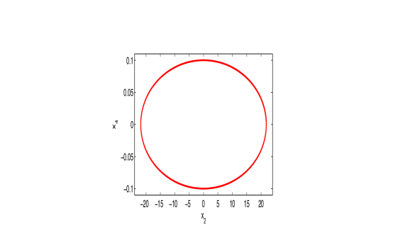
Figure 3: (Color online) A periodic limit cycle in the low-dimensional model for $k=1.5,N=6$ and $E_{0}=2$, showing that the three-wave dynamics is stable.

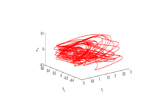
Figure 4: (Color online) A chaotic phase portrait in the low-dimensional model for $k=0.5,N=6$ and $E_{0}=2$, showing that the three-wave dynamics is unstable.

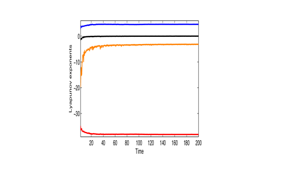
Figure 5: (Color online) The four Lyapunov exponents with respect to time $(t\epsilon)$ corresponding to the same parameter values as in Fig. 4. One of the exponents is clearly positive, indicating that the three-wave dynamics is chaotic.

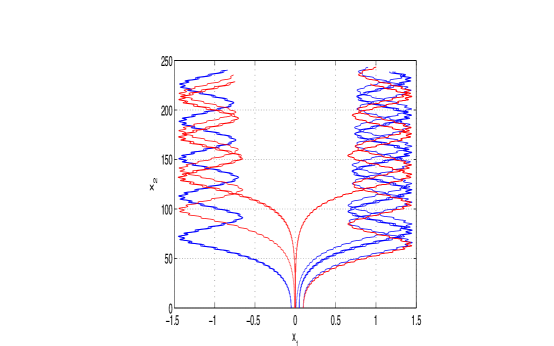
Figure 6: (Color online) Supercritical Hopf-bifurcation in the low-dimensional model for $k=0.45,N=7$ and $E_{0}=2$, showing the bifurcation of an attracting periodic orbit.

Thus, when $k<k_{c}/2,$ the system’s periodicity breaks down. This is expected, since for smaller $k$, the solitons get more affected by the ion-acoustic radiation until they are completely destroyed. In the strong chaotic process one can expect that solitons will deliver their energy to the remaining modes so as to gradually  disappear after some time. However, one can no longer rely on the low-dimensional model for some smaller values of $k$, as it gives rise an excitation of large number of unstable harmonic modes. This is the situation where full simulation of Eqs. (5) and (6) will give better understanding for the interaction.

In addition to the above results, one interesting can also be to study the existence of Hopf-bifurcation in the Eqs. (17)-(20) by choosing $k$ as the bifurcation parameter. Generally, Hopf-bifurcation is defined as the change in qualitative behavior of the system when a pair of complex conjugate eigenvalues passes through the imaginary axis. A pair of such roots can be obtained by numerically examining the eigenvalue equation (25).  Thus, one can perform a series of analysis with different values of $k$. Figure 6 shows the supercritical diagram corresponding to $N=7$ and $k=0.45$ in which an attracting periodic orbit bifurcates. The detailed analysis of such bifurcation is, however, beyond the scope of the present work.

V Simulation results for the spatiotemporal evolution

In the previous section we have observed that as the value of $k$ is lowered from $k_{c}/2,$ the system exhibits strong chaotic features. So, in order to investigate the global behaviors of the solitons, namely the soliton interaction with strong IAW emission, formation of incoherent patterns due to collision and fusion, it is reasonable to consider the system of Eqs. (5) and (6) without the mixed derivatives (valid for long-wavelengths). In our numerical scheme, we assume the spatial periodicity with the simulation box length $L_{x}$ such that $L_{x}=2\pi/k,$ the resonant wave length. The integer $M=[k^{-1}],$ representing the number of modes, is considered as a number of grid points, e.g., $256,512,1024$ and $2048$ as the case may be. We choose the initial conditions as Misra2 ; He

$$E(x,0) =E_{0}\left[1+b\cos(kx)/L\right],$$

$$\text{ }n(x,0) =-2bE_{0}\cos(kx)/L,$$ (29)

where $E_{0}$ is the amplitude of the pump Langmuir wave, $b$ is a suitable constant, and $L$ is of the order of $10^{-3}$ to emphasize that the perturbation is relatively small. The spatiotemporal system was advanced in time using the Runge-Kutta scheme with a time step $dt=0.001$. We consider the grid size $M=2048$ for lower values of $k$, and $M=1024$ for relatively large $k,$ so that $x=0$ corresponds to the grid position $1024$ and $512$ respectively. In the simulation, we consider $E_{0}=2,$ $b=1\$and $\epsilon=\sqrt{1/1840}$, unless otherwise mentioned.

Figures 7 (in presence of IWN) and 8 (in absence of IWN) show the profiles of the electric filed (upper panel) and density fluctuation (lower panel) associated with the IAWs at the end of simulation for $k=0.22,$ i.e., for the of $M\equiv[k^{-1}]=4$ harmonic modes. At the central part, we observe an excited electric field, $|E|\sim 9.5\epsilon$ highly correlated with the density depletion, $\nu=-81.2\epsilon^{2}$ in presence of IWN. Whereas in absence of IWN, these are $|E|\sim 9.375\epsilon$ and $\nu=-84.4\epsilon^{2}.$ Clearly, the effect of IWN is to enhance the magnitude of the wave electric field or to decrease that of the density fluctuation.  From Fig. 9 (contour plot corresponding to Fig. 7), we observe that the solitary master patterns are first formed by the master mode, and then begin to appear from the unstable harmonic modes. During the pattern formation, ions are usually driven out (by the resultant of ponderomotive force and the IWN) from the regions of the master mode as well as from some harmonic patterns, and then they form density distributions with $\nu>0$ (see the lower panels of Figs. 7 and 8) along the spatial axis. These ion density humps move stochastically on either side of the patterns, and do not arrest the Langmuir wave fields. We observe from Figs. 9 and 10 (contour plot corresponding to Fig. 8) that the pattern selection leads to three $(<M=4)$ harmonic modes initially peaked at $x=L_{x}/4\epsilon,L_{x}/2\epsilon$ and $3L_{x}/4\epsilon.$ These three modes are basically generated by the master mode and the unstable harmonic modes. The system is then in the coexistence of temporal chaos (TC) and spatio-partial coherence (SPC) state similar to the case of plane wave region $(k_{c}/2<k<k_{c})$ explained in the previous section.

However, as the IWN is relaxed, only two solitary patterns initially peaked at $x=L_{x}/4\epsilon$ and $3L_{x}/4\epsilon$ are seen to collide with the master mode at $t\approx 120/\epsilon$ and $t\approx 170/\epsilon$ respectively (see Fig. 10). Also, the collision is so weak that it does not influence the soliton dynamics. The reason is that in absence of IWN and for relatively small $E_{0}$, the ponderomotive force was the only force to cause the weak ion-acoustic wave emission. As a result, though the collisions take place but are not sufficiently strong to fuse into a new one. On the other hand, when $E_{0}$ is relatively large, e.g., $E_{0}=4,$ i.e., when the amplitude of both the initial profiles increase, one may observe (see Fig. 11) more collision and fusion due to strong IAW emission by the IWN. In this case, $|E|$ increases, but $|\nu|$ decreases as compared to the case of no IWN (Fig. 12).  Figure 11 also shows that two pairs of solitary patterns initially peaked at the either side of $x\approx 256/\epsilon,$ collide and fuse into two new patterns, one of which again collides with the other two master patterns peaked at $x\approx 256/\epsilon$ and $x\approx 465/\epsilon$ at $t\approx 115/\epsilon$ and $165/\epsilon.$ After these collisions, there remain only three distorted patterns. The system is in TC, but still in the coexistence of TC and STC, since a few collisions will not suffice to cause STC He .

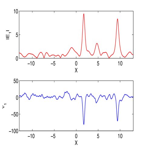
Figure 7: (Color online) The profiles of the wave electric field ($|E_{1}|\equiv|E|/\epsilon,$ upper panel) and the associated density fluctuation ($\nu_{1}\equiv\nu/\epsilon^{2},$ lower panel) with respect to the space $(X\equiv x\epsilon)$ after time $t=200/\epsilon$ in the numerical simulation of Eqs. (5) and (6) for $k=0.22$ and $E_{0}=2$ with IWN.

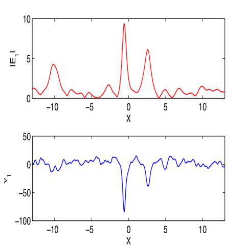
Figure 8: (Color online) The same as in Fig. 7, but without IWN.

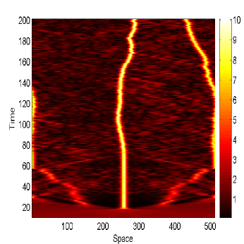
Figure 9: (Color online) Contours of $|E(x,t)|=$const. with respect to the space $(x\epsilon)$ and time $(t\epsilon)$ corresponding to the evolution as in Fig. 7. This shows that the pattern selection leads to three harmonic patterns. The system is in the coexistence of TC and SPC state.

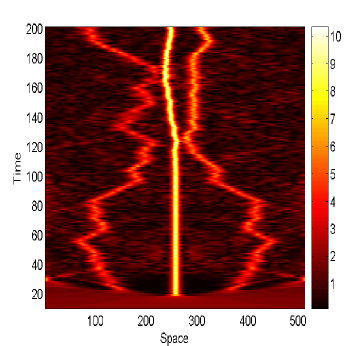
Figure 10: (Color online) Contours of $|E(x,t)|=$const. with respect to the space $(x\epsilon)$ and time $(t\epsilon)$ corresponding to the evolution as in Fig. 8. This shows that the pattern selection leads to three harmonic patterns. Two collisions occur at $t\approx 120/\epsilon$ and $t\approx 170/\epsilon.$ The system is still in the coexistence of TC and SPC state.

Now, if $k$ is further lowered, e.g., $k=0.065,$ many solitary patterns are formed from the master mode and unstable harmonic modes (see Fig. 13 with IWN and Fig. 14 without IWN) by means of pattern selection. We observe that when IWN influences the dynamics, many unstable harmonic modes are excited compared to the other case. As a result, not only two solitary patterns collide (as mostly in the case of no IWN) to fuse into a new pattern, but more than two also collide repeatedly to form new ones which again collide with other new pattern(s) fused by the other collisions. Notice from Figure 13 that the first collision occurs at $t\approx 57/\epsilon$ between two solitary patterns. These two patterns then fuse to form a new one, which again collides with other three master patterns initially peaked at $x\approx 190/\epsilon,$ $325/\epsilon$ and $700/\epsilon$ at $t\approx 95/\epsilon,120/\epsilon$ and $150/\epsilon$ respectively. There are also other collision and fusion that can be explained similarly. In general, as time progresses, the patterns seem to be much distorted in losing their strengths. The original $17$ (Fig. 13) or $15$ (Fig. 14) solitary patterns are then finally fused into a few incoherent ones. As solitons gradually vanish, irregular radiation increases due to stochastic motion. That is, as soon as a chaotic subset with less degrees of freedom is formed, the subset will then act as a pump delivering a net amount of energy to its neighboring modes. This energy transfer takes place because of the very random nature of the couplings. The system is then said to be in the STC state. In this case, for $t>100/\epsilon$ the spatial correlation function will approach to a zero value  He . A certain amount of energy, which was initially distributed among the $15$ or $17$ solitary waves, will now be transferred to a few incoherent patterns as well as to some stable higher harmonic modes with short-wavelengths.

So, if initially there exist many modulational unstable modes with different modulation lengths to form solitary envelopes, collision and fusion among most of them can lead to the state of STC. There must exist a critical value of this wavelength or wave number $k$ at which the transition from TC to STC takes place. This value of $k$ is roughly in $0.03<k<0.1.$ Comparing the pattern formation, collision and fusion in Figs. 11, 12 and 13, 14 one finds that IAW emission is more stronger in presence of IWN. Thus, in order to observe the interactions between LWs and IAWs at longer time scale and for long-wavelength limits, the effect of IWN is more important, which can no longer be neglected especially for relatively large amplitude waves. In this way, the term containing the IWN in Eq. (2) would act as a correction to the dynamics of arbitrary amplitude coupled Langmuir and IAWs.

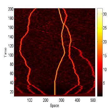
Figure 11: (Color online) The same as in Fig. 9 for $k=0.22$, but for relatively large $E_{0}$, i.e., $E_{0}=4$, indicating that more collision and fusion take place due to IWN.

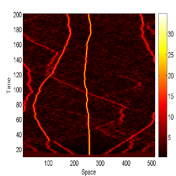
Figure 12: (Color online) The same as in Fig. 11, but in absence of IWN, indicating that relatively a less number of collision and fusion take place compared to Fig. 11.

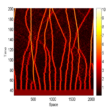
Figure 13: (Color online) Contours of $|E(x,t)|=$const. with respect to the space $(x\epsilon)$ and time $(t\epsilon)$ for $k=0.065$ and $E_{0}=2$ in presence of IWN. The pattern selection shows that seventeen solitary patterns, which were  formed initially, collide and get fused into other incoherent patterns after some time. The collision is random and not confined between two patterns. The IAW emission also occurs, and the STC state emerges.

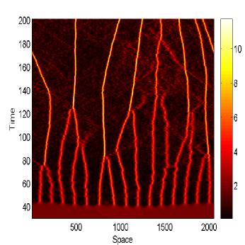
Figure 14: (Color online)  The same as in Fig. 13, but in absence of IWN. Notice that fifteen solitary patterns were formed initially. After some time they collide and fuse to form several new incoherent patterns. Here the collision is mostly between two patterns compared to Fig. 13. The STC state is also said to emerge in this case.

VI Discussion and conclusion

From the analysis of the previous sections, we find that the three-wave model can be a good approximation Rizzato for the interaction of coupled LWs and IAWs in the plane wave region $k_{c}/2<k<k_{c},$ where the system exhibits stable oscillations. It can relatively be accurate in the region $0.3\lesssim k<k_{c}/2$ where the system exhibits temporal chaos for a given value of the pump electric field $E_{0}$. For values of $k<0.3,$ which indicates the excitation of many ($>3$) unstable harmonic modes, the low-dimensional model fails to describe the dynamics of the coupled waves. We have found that the three-wave model exhibits periodic orbits in $1.2\lesssim k<k_{c},$and chaos in $0.3\lesssim k\lesssim 0.5<k_{c}/2$ for a given initial pump $E_{0}=2$ and a given constant $N=6.$ The space-time evolution, on the other hand, reveals that the system is in the state of TC for relatively a lower value of $k,$ i.e., in the regime $0.1\lesssim k\lesssim 0.22,$ and the STC state emerges for $0.03<k<0.1.$

To conclude, we have investigated the nonlinear interaction of coupled LWs and IAWs by considering the effects of dispersion due to charge separation, and the nonlinearity associated with the ion density fluctuations. The latter can cause the excitation of more unstable harmonic modes, and can lead to strong IAW emission in the space-time evolution. The low-dimensional model shows that a transition from periodicity to chaos is possible for a suitable choice of the wave number of modulation. It basically predicts some basic features of the system as well as suggests an approximate region of $k$ for the existence of regular and chaotic structures. The space-time evolution indicates that  solitary patterns are first formed by the unstable harmonic modes. These modes are then excited by a master mode due to initial MI.  As solitons experience oscillatory motions, they emit radiation due to irregular interaction with the ion-acoustic fields. Such radiations are broad-band in nature, causing a growing number of modes to be involved in the stochastic dynamics. Depending on the modulation length scale, the system may either be in the TC and SPC states or in TC and STC states. If few harmonic patterns coexist with the master pattern, and IAW emission remains weak, the system is still in the state of TC and SPC. However, if many solitary patterns are formed at the early stage due to MI, the system may experience  the state of SPC. Over longer time scales, when solitons are affected by the free ion-acoustic radiation, collision and fusion among the patterns occur frequently as well as repeatedly to form several new incoherent patterns. The STC state is then said to emerge in which energy can flow faster the smaller is the wave number of modulation $k$. Since our model is in one spatial dimension, energy transfer is not a result of soliton collapse, rather it is purely generated by the nonintegrable nature as well as chaotic aspects of the system Rizzato . The results may have physical significance to related problems, such as turbulence in pulsar radiation where strong magnetic field plays an important role Yu .

S. B. is thankful to M.Pizzi of Micro and Nanotechnology Division, Techfab s.r.l., Chivasso, Italy, for some useful discussion. A. P. M. gratefully acknowledges support from the Kempe Foundations, Sweden.

References

- (1) V. E. Zakharov, Sov. Phys. J. Exp. Theor. Phys. 35, 908 (1972).
- (2) V. I. Karpman, H. Schamel, Phys. Plasmas 4, 120 (1997).
- (3) V. I. Karpman, Phys. Plasmas 5, 932 (1998).
- (4) P. Deeskow, H. Schamel, N. N. Rao, M. Y. Yu, R. K. Varma, and P. K. Shukla, Phys. Fluids 30, 2703 (1987).
- (5) H. Schamel and P. K. Shukla, Phys. Rev. Lett. 36, 968 (1976).
- (6) H. Schamel, M. Y. Yu, and P. K. Shukla, Phys. Fluids 20, 1286 (1977).
- (7) L. R. Hadžievski, M. M. Škorić, M. Kono, and T. Sato, Phys. Lett. A 248, 247 (1998).
- (8) G. D. Doolen, D. F. DuBois, and H. A. Rose, Phys. Rev. Lett. 54, 804 (1984).
- (9) R. Fedele, P. K. Shukla, M. Onorato, D. Anderson, M. Lisak, Phys. Lett. A 303, 61 (2002).
- (10) F. D. Prado, D. M. Karfidov, M. V. Alves, and R. S. Dallaqua, Phys. Lett. A 248, 86 (1998).
- (11) A. P. Misra, D. Ghosh, and A. R. Chowdhury, Phys. Lett. A 372, 1469 (2008).
- (12) A. P. Misra and P. K. Shukla, Phys. Rev. E 79, 056401 (2009).
- (13) A. P. Misra, S. Banerjee, F. Haas, P. K. Shukla, L. P. G. Assis, Phys. Plasmas 17, 032307 (2010).
- (14) A. C. -L. Chain, S. R. Lopes, and J. R. Abalde, Physica D 99, 269 (1996).
- (15) K. Batra, R. P. Sharma and A. D. Verga, J. Plasma Phys. 72, 671 (2006).
- (16) F. B. Rizzato, G. I. de Oliveria, and R. Erichsen, Phys. Rev. E, 57, 2776 (1998).
- (17) M. Pettini and M. Landolfi, Phys. Rev. A 41, 768 (1990).
- (18) G. Tsaur and J. Wang, Phys. Rev. E 54, 4657 (1995).
- (19) X. T. He, C. Y. Zheng, and S. P. Zhu, Phys. Rev. E 66, 037201 (2002), and the references therein.
- (20) V. G. Makhankov, Phys. Lett. A 50, 42 (1974).
- (21) K. Nishikawa, H. Hojo, K. Mima, and H. Ikezi, Phys. Rev. Lett. 33, 148 (1974).
- (22) H. Ikezi, K. Nishikawa, and K. Mima, J. Phys. Soc. Jpn 37, 766 (1974).
- (23) G. I. de Oliveria, L. P. L. de Oliveria, and F. B. Rizzato, Phys. Rev. E 54, 3239 (1996)
- (24) M. Y. Yu, P. K. Shukla, and L. Stenflo, Astrophys. J. 309, L63 (1986).