On the Capacity of Non-Coherent
Network Coding

Abstract

We consider the problem of multicasting information from a source to a set of receivers over a network where intermediate network nodes perform randomized network coding operations on the source packets. We propose a channel model for the non-coherent network coding introduced by Koetter and Kschischang in [6], that captures the essence of such a network operation, and calculate the capacity as a function of network parameters. We prove that use of subspace coding is optimal, and show that, in some cases, the capacity-achieving distribution uses subspaces of several dimensions, where the employed dimensions depend on the packet length. This model and the results also allow us to give guidelines on when subspace coding is beneficial for the proposed model and by how much, in comparison to a coding vector approach, from a capacity viewpoint. We extend our results to the case of multiple source multicast that creates a virtual multiple access channel.

Keywords

Network coding, non-coherent communication, subspace coding, channel capacity, multi-source multicast, randomized network coding.

I Introduction

The network coding techniques for information transmission in networks introduced in [1] have attracted significant interest in the literature, both because of posing theoretically interesting questions, as well as because of potential impact in applications. The first fundamental result proved in network coding, and perhaps still the most useful from a practical point of view today, is that, using linear network coding [2, 3], one can achieve rates up to the common min-cut value when multicasting to $N_{r}\geq 1$ receivers. In general this may require operations over a field of size approximately $\sqrt{N_{r}}$, which translates to communication using packets of length $\frac{1}{2}\log N_{r}$ bits [4].

However, this result assumes that the receivers know perfectly the operations that the network nodes perform. In large dynamically changing networks, collecting network information comes at a cost, as it consumes bandwidth that could instead have been used for information transfer. In practical networks, where such deterministic knowledge is not sustainable, the most popular approach is to perform randomized network coding [5] and to append coding vectors at the headers of the packets to keep track of the linear combinations of the source packets they contain (see, e.g., [12]). The coding vectors have an overhead of $h\log N_{r}$ bits, where $h$ is the total number of packets to be linearly combined. This results in a loss of information rate that can be significant with respect to the min-cut value. In particular, in wireless networks such as sensor networks where communication is restricted to short packet lengths, the coding vector overhead can be a significant fraction of the overall packet length [27, 13].

Use of coding vectors is akin to use of training symbols to learn the transformation induced by a network. A different approach is to assume a non-coherent scenario for communication, as proposed in [6], where neither the source(s) nor the receiver(s) have any knowledge of the network topology or the network nodes operations. Non-coherent communication allows for creating end-to-end systems completely oblivious to the network state. Several natural questions arise considering this non-coherent framework: (i) what are the fundamental limits on the rates that can be achieved in a network where the intermediate node operations are unknown, (ii) how can they be achieved, and (iii) how do they compare to the coherent case.

In this work we address such questions for two different cases. First, we consider the scenario where a single source aims to transmit information to one or multiple receiver(s) over a network under the non-coherence assumption using fixed packet length. Because network nodes only perform linear operations, the overall network behavior from the source(s) to a receiver can be represented as a matrix multiplication of the sent source packets. We consider operation in time-slots, and assume that the channel transfer matrices are distributed uniformly at random and i.i.d. over different time-slots. Under this probabilistic model, we characterize the asymptotic capacity behavior of the introduced channel and show that using subspace coding we can achieve the optimal performance. We extend our model for the case of multiple sources and characterize the asymptotic behavior of the optimal rate region for the case of two sources. We believe that this result can be extended to the case of more than two sources using the same method that is applied in §V. For the multi-source case we prove as well that encoding information using subspaces is sufficient to achieve the optimal rate region.

The idea of non-coherent modeling for randomized network coding was first proposed in the seminal work by Koetter and Kschischang in [6]. In that work, the authors focused on algebraic subspace code constructions over a Grassmannian. Independently and in parallel to our work in [9], Montanari et al. [14] introduced a different probabilistic model to capture the end-to-end functionality of non-coherent network coding operation, with a focus on the case of error correction capabilities. Their model does not examine subsequent time slots, but instead, allows the packets block length (in this paper terminology; packet length $T$) to increases to infinity, with the result that the overhead of coding vectors becomes negligible, very fast.

Silva et al. [16] independently and subsequent to our works in [9] and [10], also considered a probabilistic model for non-coherent network coding, which is an extension of the model introduced in [14] over multiple time-slots. In their model the transfer matrix is constrained to be square as well as full rank. This is in contrast to our model, where the transfer matrix can have arbitrary dimensions, and the elements of the transfer matrix are chosen uniformly at random, with the result that the transfer matrix itself may not have full rank (this becomes more pronounced for small matrices). Moreover, we extend our work to multiple source multicast, which corresponds to a virtual non-coherent multiple access channel (MAC). Our results coincide for the case of a single source, when the packet length and the finite field of operations are allowed to grow sufficiently large. Another difference is that the work in [16] focuses on additive error with constant dimensions; in contrast, we focus on packet erasures.

An interpretation of our results is that it is the finite field analog of the Grassmannian packing result for non-coherent MIMO channels as studied in the well known work in [19]. In particular, we show that for the non-coherent model over finite fields, the capacity critically depends on the relationship between the “coherence time” (or packet length $T$ in our model) and the min-cut of the network. In fact the number of active subspace dimensions depend on this relationship; departing from the non-coherent MIMO analogy of [19].

The paper is organized as follows. We define our notation and channel model in §II; we state and discuss our main results in §III; we prove the capacity results for the single and multiple sources in sections §IV and §V respectively; and conclude the paper in §VI.

All the missing proofs for lemmas, theorems, and etc., are given in Appendix A unless otherwise stated.

II Channel Model and Notation

II-A Notation

We here introduce the notation and definitions we use in the following sections. Let $q\geq 2$ be a power of a prime. In this paper, all vectors and matrices have elements in a finite field $\mathbb{F}_{q}$. We use $\mathbb{F}^{n\times m}_{q}$ to denote the set of all $n\times m$ matrices over $\mathbb{F}_{q}$, and $\mathbb{F}^{T}_{q}$ to denote the set of all row vectors of length $T$. The set $\mathbb{F}_{q}^{T}$ forms a $T$-dimensional vector space over the field $\mathbb{F}_{q}$.

Throughout the paper, we use capital letters, e.g., $X$, to denote random objects, including random variables, random matrices, or random subspaces, and corresponding lower-case letters, e.g., $x$ to denote their realizations. For example, we denote by $\Pi$ a “random subspace” which takes as values the subspaces in a vector space according to some distribution, and by $\pi$ a specific realization. Also, bold capital letters, e.g., $\mathbf{A}$, are reserved for deterministic matrices and bold lower-case letters, e.g., $\mathbf{v}$, are used for deterministic vectors.

For subspaces $\pi_{1}$ and $\pi_{2}$, $\pi_{1}\sqsubseteq\pi_{2}$ denotes that $\pi_{1}$ is a subspace of $\pi_{2}$. Recall that for two subspaces $\pi_{1}$ and $\pi_{2}$, $\pi_{1}\cap\pi_{2}$ is the intersection of these subspaces which itself is a subspace. We use $\pi_{1}+\pi_{2}$ to denote the smallest subspace that contains both $\pi_{1}$ and $\pi_{2}$, namely,

$$\pi_{1}+\pi_{2}=\left\{\mathbf{v}_{1}+\mathbf{v}_{2}|\mathbf{v}_{1}\in\pi_{1},\mathbf{v}_{2}\in\pi_{2}\right\}.$$

It is well known that

$$\dim(\pi_{1}+\pi_{2})=\dim(\pi_{1})+\dim(\pi_{2})-\dim(\pi_{1}\cap\pi_{2}).$$

For a set of vectors $\{\mathbf{v}_{1},\ldots,\mathbf{v}_{k}\}$ we denote their linear span by $\left\langle\mathbf{v}_{1},\dots,\mathbf{v}_{k}\right\rangle$. For a matrix $\mathbf{X}$, $\left\langle\mathbf{X}\right\rangle$ is the subspace spanned by the rows of $\mathbf{X}$ and $\left\langle\mathbf{X}\right\rangle_{c}$ is the subspace spanned by the columns of $\mathbf{X}$. We then have $\mathrm{rank}(\mathbf{X})=\dim(\left\langle\mathbf{X}\right\rangle)=\dim(\left\langle\mathbf{X}\right\rangle_{c})$.

We use the calligraphic symbols, i.e., $\mathcal{X}$ or $\mathcal{Y}$ to denote a set of matrices. To denote a set of subspaces we use the same calligraphic symbols but with a “$\sim$”, i.e., $\widetilde{\mathcal{X}}$ or $\widetilde{\mathcal{Y}}$.

We use the symbols “$\succ$” and “$\prec$” to denote the element-wise inequality between vectors and matrices of the same size.

For two real valued functions $f(x)$ and $g(x)$ of $x$, we use $f(x)\doteq g(x)$ to denote that

$$\lim_{x\rightarrow\infty}\frac{\log f(x)}{\log g(x)}\rightarrow 1.$$

Note that the definition of “$\doteq$” is different from the more standard definition which is $\lim_{x\to\infty}\frac{1}{x}\log\frac{f(x)}{g(x)}\to 0$. We also use a similar definition for $f\stackrel{{\scriptstyle.}}{{\leq}}g$ to denote that

$$\lim_{x\rightarrow\infty}\frac{\log f(x)}{\log g(x)}\rightarrow c\leq 1,$$

where $c$ is a constant.

We use the big-$O$ notation which is defined as follows. Let $f(x)$ and $g(x)$ be two functions defined on some subset of the real numbers. We write $f(x)=O\left(g(x)\right)\mbox{ as }x\to\infty,$ if there exists a positive real number $M$ and a real number $x_{0}$ such that $|f(x)|\leq M|g(x)|\mbox{ for all }x>x_{0}.$ For the little $o$ notation we use the following definition. We write $f(x)=o(g(x))\mbox{ as }x\to\infty,$ if for all $\epsilon>0$ there exists a real number $x_{0}$ such that $|f(x)|\leq\epsilon\cdot|g(x)|\mbox{ for all }x>x_{0}.$ We use also the big-$\Omega$ notation which is defined as follows. We write $f(x)=\Omega\left(g(x)\right)\mbox{ as }x\to\infty,$ if we have $g(x)=O\left(f(x)\right)\mbox{ as }x\to\infty$. Finally, we use the big-$\Theta$ notation to denote that a function is bounded both above and below by another function asymptotically. Formally, we write $f(x)=\Theta\left(g(x)\right)\mbox{ as }x\to\infty,$ if and only if we have $f(x)=O\left(g(x)\right)$ and $f(x)=\Omega\left(g(x)\right)\mbox{ as }x\to\infty$.

Definition 1 (Grassmannian and Gaussian coefficient [22, 25])

The Grassmannian $\mathrm{Gr}(T,d)_{q}$ is the set of all $d$-dimensional subspaces of the $T$-dimensional space over a finite field $\mathbb{F}_{q}$, namely,

$$\mathrm{Gr}(T,d)_{q}\triangleq\{\pi\sqsubseteq\mathbb{F}_{q}^{T}:\dim(\pi)=d\}.$$

The cardinality of $\mathrm{Gr}(T,d)_{q}$ is the Gaussian coefficient, namely,

$${T\brack d}_{q} \triangleq|\mathrm{Gr}(T,d)_{q}|=\frac{(q^{T}-1)\cdots(q^{T-d+1}-1)}{(q^{d}-1)\cdots(q-1)}.$$ (1)

Definition 2 (The set $\mathrm{Sp}(T,m)_{q}$)

We define $\mathrm{Sp}(T,m)_{q}$ to be the set (sphere) of all subspaces of dimension at most $m$ in the $T$-dimensional space $\mathbb{F}_{q}^{T}$, namely

$$\mathrm{Sp}(T,m)_{q}\triangleq\bigcup_{d=0}^{\min[m,T]}\mathrm{Gr}(T,d)_{q}=\{\pi\sqsubseteq\mathbb{F}_{q}^{T}:\dim(\pi)\leq\min[m,T]\}.$$

The cardinality of $\mathrm{Sp}(T,m)_{q}$ equals

$$\mathcal{S}(T,m)_{q}\triangleq|\mathrm{Sp}(T,m)_{q}|=\sum_{d=0}^{\min[m,T]}|\mathrm{Gr}(T,d)_{q}|.$$

Definition 3 (The number $\psi(T,n,\pi_{d})_{q}$ )

We denote by $\psi(T,n,\pi_{d})_{q}$ the number of different $n\times T$ matrices with elements from a field $\mathbb{F}_{q}$, such that their rows span a specific subspace $\pi_{d}\sqsubseteq\mathbb{F}_{q}^{T}$ of dimension $0\leq d\leq\min[n,T]$.

For simplicity, in the rest of the paper we will drop the subscript $q$ in the previous definitions whenever it is obvious from the context.

II-B Preliminary Lemmas

We here state some preliminary lemmas related to the definitions introduced in §II-A.

Existing bounds in the literature allow to approximate the Gaussian number, for example, we have from [6, Lemma 4] that [23, Section III]

$$q^{d(T-d)}<{T\brack d}<\frac{q^{d(T-d)}}{\prod_{j=1}^{\infty}(1-q^{-j})}<4q^{d(T-d)},\quad\forall d:0<d<T.$$ (2)

Using Definition 1 and (2) we have Lemma 1.

Lemma 1

For large $q$ we can approximate the Gaussian number as follows

$${T\brack d}=q^{d(T-d)}(1+O(q^{-1}))\doteq q^{d(T-d)}.$$

Lemma 2

For $\psi(T,n,\pi_{d})$ given in Definition 3, we have that [26]

$$\psi(T,n,\pi_{d})=\prod_{i=0}^{d-1}(q^{n}-q^{i})=q^{\binom{d}{2}}\prod_{i=0}^{d-1}(q^{n-i}-1),$$

i.e., it does not depend on $T$.

Since $\psi(T,n,\pi_{d})$ does not depend on $T$, and only depends on $\pi_{d}$ through its dimension, as a shorthand notation we will also use $\psi(n,d)$ instead of $\psi(T,n,\pi_{d})$, where $d=\dim(\pi_{d})$.

Using Lemma 2 the following lower and upper bounds are straightforward

$$(1-dq^{-n+d-1})<\left(1-\sum_{i=0}^{d-1}q^{-n+i}\right)<\frac{\psi(n,d)}{q^{nd}}<1,$$ (3)

which imply Lemma 3 (see also [23]).

Lemma 3

For large values of $q$ the following approximation holds

$$\psi(n,d)=q^{nd}(1+O(q^{-1}))\doteq q^{nd}.$$

It is also worthwhile to mention that $\psi(n,d){T\brack d}$ is the number of $n\times T$ matrices of rank $d$. We can count all the $n\times T$ matrices through the following Lemma 4, (also see [22, 25], and [26, Corollary 5]).

Lemma 4

For every $n>0$ and $T>0$ we can write

$$\sum_{d=0}^{\min[n,T]}\psi(n,d){T\brack d}=q^{nT},$$

where $\psi(n,0)=1$.

II-C The Non-Coherent Finite Field Channel Model

We consider a network where nodes perform random linear network coding over a finite field $\mathbb{F}_{q}$. We are interested in the maximum information rate at which a single (or multiple) source(s) can successfully communicate over such a network when neither the transmitter nor the receiver(s) have any channel state information (CSI). For simplicity, we will present the channel model and our analysis for the case of a single receiver; the extension to multiple receivers (with the same channel parameters) is straightforward, as we also discuss in the results section.

We assume that time is slotted and the channel is block time-varying. For the single source communication, at time slot $t$, the receiver observes

$$Y[t]=G[t]X[t],$$ (4)

where $X[t]\in\mathbb{F}_{q}^{m\times T}$, $G[t]\in\mathbb{F}_{q}^{n\times m}$, and $Y[t]\in\mathbb{F}_{q}^{n\times T}$. At each time-slot, the receiver receives $n$ packets of length $T$ (captured by the rows of matrix $Y[t]$) that are random linear combinations of the $m$ packets injected by the source (captured by the rows of matrix $X[t]$). In our model, the packet length $T$ can be interpreted as the coherence time of the channel, during which the transfer matrix remains constant. Each element of the transfer matrix $G[t]$ is chosen uniformly at random from $\mathbb{F}_{q}$, changes independently from time slot to time slot, and is unknown to both the source and the receiver. In other words, the channel transfer matrix is chosen uniformly at random from all possible matrices in $\mathbb{F}_{q}^{n\times m}$ and has i.i.d. distribution over different blocks. In general, the topology of the network may impose some constraints on the transfer matrix $G[t]$ (for example, some entries might be zero, see [3, 8, 20, 21]). However, we believe that this is a reasonable general model, especially for large-scale dynamically-changing networks where apart from random coefficients there exist many other sources of randomness. Formally, we define the non-coherent matrix channel as follows.

Definition 4 (Non-coherent matrix channel $\mathrm{Ch}_{\textsl{m}}$)

This is defined to be the matrix channel $\mathrm{Ch}_{\textsl{m}}:\mathcal{X}\rightarrow\mathcal{Y}$ described by (4) with the assumption that $G[t]$ is i.i.d. and uniformly distributed over all matrices $\mathbb{F}_{q}^{n\times m}$. It is a discrete memoryless channel with input alphabet $\mathcal{X}\triangleq\mathbb{F}_{q}^{m\times T}$ and output alphabet $\mathcal{Y}\triangleq\mathbb{F}_{q}^{n\times T}$.

The capacity of the channel $\mathrm{Ch}_{\textsl{m}}$ is given by

$$C_{\textsl{m}}=\max_{P_{X}(x)}I(X;Y),$$ (5)

where $P_{X}(x)$ is the input distribution. To achieve the capacity a coding scheme may employ the channel given in (4) multiple times, and a codeword is a sequence of input matrices from $\mathcal{X}$. For a coding strategy that induces an input distribution $P_{X}(x)$, the achievable rate is

$$R=I(X;Y).$$

Now we define a non-coherent subspace channel $\mathrm{Ch}_{\textsl{s}}$ which takes as an input a subspace and outputs another subspace. Then, in Theorem 1 we will show that the two channels $\mathrm{Ch}_{\textsl{m}}$ and $\mathrm{Ch}_{\textsl{s}}$ are equivalent from the point of view of calculating the mutual information between their inputs and their outputs.

Definition 5 (Non-coherent subspace channel $\mathrm{Ch}_{\textsl{s}}$)

This is defined to be the channel $\mathrm{Ch}_{\textsl{s}}:\widetilde{\mathcal{X}}\rightarrow\widetilde{\mathcal{Y}}$ with input alphabet $\widetilde{\mathcal{X}}=\mathrm{Sp}(T,m)$ and output alphabet $\widetilde{\mathcal{Y}}=\mathrm{Sp}(T,n)$ and transition probability

$$P_{\Pi_{Y}|\Pi_{X}}(\pi_{y}|\pi_{x})\triangleq\left\{\begin{array}[]{ll}\psi(T,n,\pi_{y})q^{-n\dim(\pi_{x})}&\pi_{y}\sqsubseteq\pi_{x},\\ 0&\text{otherwise},\end{array}\right.$$ (6)

where $\Pi_{X}$ and $\Pi_{Y}$ are the input and output variables of the channel $\mathrm{Ch}_{\textsl{s}}$.

The capacity of the channel $\mathrm{Ch}_{\textsl{s}}$ is given by

$$C_{\textsl{s}}=\max_{P_{\Pi_{X}}(\pi_{x})}I(\Pi_{X};\Pi_{Y}),$$

where $P_{\Pi_{X}}(\pi_{x})$ is the input distribution defined over the set of subspaces $\widetilde{\mathcal{X}}$.

We next consider a multiple sources scenario, and the multiple access channel corresponding to (4). In this case, we have

$$Y[t]=\sum_{i=1}^{N_{s}}G_{i}[t]X_{i}[t],$$ (7)

where $N_{s}$ is the number of sources, and each source $i$ inserts $m_{i}$ packets to the network. Thus, $X_{i}[t]\in\mathbb{F}_{q}^{m_{i}\times T}$, $G_{i}[t]\in\mathbb{F}_{q}^{n\times m_{i}}$ and $Y[t]\in\mathbb{F}_{q}^{n\times T}$. We can also collect all $G_{i}[t]$ in an $n\times\sum_{i=1}^{N_{s}}m_{i}$ matrix $G_{\textsl{MAC}}[t]$ and all $X_{i}[t]$ in an $\sum_{i=1}^{N_{s}}m_{i}\times T$ matrix $X_{\textsl{MAC}}[t]$ as following

$$X_{\textsl{MAC}}[t]=\left[\begin{array}[]{c}X_{1}[t]\\ \vdots\\ X_{N_{s}}[t]\\ \end{array}\right],\quad\text{and}\quad G_{\textsl{MAC}}[t]=\left[\begin{array}[]{ccc}G_{1}[t]&\cdots&G_{N_{s}}[t]\end{array}\right],$$

so we can rewrite (7) as

$$Y[t]=G_{\textsl{MAC}}[t]X_{\textsl{MAC}}[t].$$

Each source $i$ then controls $m_{i}$ rows of the matrix $X_{\textsl{MAC}}[t]$. Again we assume that each entry of the matrices $G_{i}[t]$ is chosen i.i.d. and uniformly at random from the field $\mathbb{F}_{q}$ for all source nodes and all time instances.

Definition 6 (The non-coherent multiple access matrix channel $\mathrm{Ch}_{\textsl{m-MAC}}$)

This is defined to be the channel $\mathrm{Ch}_{\textsl{m-MAC}}:\mathcal{X}_{1}\times\cdots\times\mathcal{X}_{N_{s}}\rightarrow\mathcal{Y}$ described in (7), with the assumption that $G_{i}[t]$, $i=1,\ldots,N_{s}$, are i.i.d. and uniformly distributed over all matrices $\mathbb{F}_{q}^{n\times m_{i}}$, $i=1,\ldots,N_{s}$. It forms a discrete memoryless MAC with input alphabets $\mathcal{X}_{i}\triangleq\mathbb{F}_{q}^{m_{i}\times T}$, $i=1,\ldots,N_{s}$, and output alphabet $\mathcal{Y}\triangleq\mathbb{F}_{q}^{n\times T}$.

It is well known [15] that the rate region of any multiple access channel including $\mathrm{Ch}_{\textsl{m-MAC}}$ is given by the closure of the convex hull of the rate vectors satisfying

$$R_{S}\leq I(X_{S};Y|X_{S^{c}})\quad\text{for all }S\subseteq\{1,\ldots,N_{s}\},$$

for some product distribution $P_{X_{1}}(x_{1})\cdots P_{X_{N_{s}}}(x_{N_{s}})$. Note that $R_{S}=\sum_{i\in S}R_{i}$ where $R_{i}$ is the transmission rate of the $i$th source, $X_{S}=\{X_{i}:i\in S\}$ and $S^{c}$ is the complement set of $S$.

As before, we define a non-coherent subspace version of the matrix multiple access channel and in Theorem 6 we show that from the point of view of rate region these two channels are equivalent.

Definition 7 (Non-coherent subspace multiple access channel $\mathrm{Ch}_{\textsl{s-MAC}}$)

This is defined to be the channel $\mathrm{Ch}_{\textsl{s-MAC}}:\widetilde{\mathcal{X}}_{1}\times\widetilde{\mathcal{X}}_{2}\rightarrow\widetilde{\mathcal{Y}}$ with input alphabets $\widetilde{\mathcal{X}}_{i}=\mathrm{Sp}(T,m_{i})$, $i=1,2$, output alphabet $\widetilde{\mathcal{Y}}=\mathrm{Sp}(T,n)$ and transition probability

$$\Pr(\Pi_{Y}=\pi_{y}| \Pi_{X_{1}}=\pi_{1},\Pi_{X_{2}}=\pi_{2})=\left\{\begin{array}[]{ll}\psi(T,n,\pi_{y})q^{-n\dim(\pi_{1}+\pi_{2})}&\pi_{y}\sqsubseteq\pi_{1}+\pi_{2},\\ 0&\text{otherwise},\end{array}\right.$$ (10)

where $\Pi_{X_{1}}$ and $\Pi_{X_{2}}$ are the input and $\Pi_{Y}$ is the output variables of the channel $\mathrm{Ch}_{\textsl{s-MAC}}$.

III Main Results

III-A Single Source

Our main results, Theorem 2 and Theorem 3, characterize the capacity for non-coherent network coding for the model given in (4). We show that the capacity is achieved through subspace coding, where the information is communicated from the source to the receivers through the choice of subspaces. Formally, we have the following results.

Theorem 1

The matrix channel $\mathrm{Ch}_{\textsl{m}}:\mathcal{X}\rightarrow\mathcal{Y}$ defined in Definition 4 and the subspace channel $\mathrm{Ch}_{\textsl{s}}:\widetilde{\mathcal{X}}\rightarrow\widetilde{\mathcal{Y}}$ defined in Definition 5 are equivalent in terms of evaluating the mutual information between the input and output. More precisely, for every input distribution for the channel $\mathrm{Ch}_{\textsl{s}}$ there is an input distribution for the channel $\mathrm{Ch}_{\textsl{m}}$ such that $I(X;Y)=I(\Pi_{X};\Pi_{Y})$ and vice versa. As a result, these channels have the same capacity $C_{\textsl{m}}=C_{\textsl{s}}$.

For the proof of Theorem 1 refer to Appendix A and for more discussion refer to §IV-A.

Theorem 2

For the channel $\mathrm{Ch}_{\textsl{m}}:\mathcal{X}\rightarrow\mathcal{Y}$ defined in Definition 4, the capacity is given by

$$C_{\textsl{m}} =i^{*}(T-i^{*})\log_{2}q+o(1),$$ (11)

where $i^{*}=\min\left[m,n,\lfloor T/2\rfloor\right]$, and $o(1)$ tends to zero as $q$ grows.

Theorem 2 is proved in §IV-B. The result of Theorem 2 is for large alphabet regime. The following result, Theorem 3, is valid for a finite field size, and therefore is a non-asymptotic result.

Theorem 3

Consider the channel $\mathrm{Ch}_{\textsl{m}}:\mathcal{X}\rightarrow\mathcal{Y}$ defined in Definition 4. There exists a finite number $q_{0}$ such that for $q>q_{0}$ the optimal input distribution is nonzero only for matrices of rank in the set

$$\mathcal{A}=\left\{\min\left[(T-n)^{+},m,n,T\right],\ldots,\min\left[m,n,T\right]\right\}.$$ (12)

Moreover, for all values of $q$ the optimal input distribution is uniform over all matrices $X$ of the same rank, and the total probability allocated to transmitting matrices of rank $i$ equals

$$\alpha^{*}_{i}\triangleq{\mathbb{P}\left[\mathrm{rank}(X)=i\right]}=2^{-C_{\textsl{m}}}q^{i(T-i)}\left[1+o(1)\right],\quad\forall i\in\mathcal{A}.$$ (13)

The proof of Theorem 3 is presented in §IV-C and §IV-D, and uses standard techniques from convex optimization, as well as large field size approximations. Note that, the same coding scheme at the source simultaneously achieves the capacity for all receivers with the same channel parameters (i.e., values of $n$, $m$ and $T$). That is, each receiver is able to successfully decode.

The result of Theorem 3 for the active set of input dimensions is not asymptotic in $q$. However, it is not easy to analytically find the minimum value of $q_{0}$ such that the theorem statement holds for all $q>q_{0}$. Theorem 4 demonstrates how we can analytically characterize $q_{0}$ given in Theorem 3 for the case $T>n+\min[m,n]$. The proof of Theorem 4 is presented in §IV-E.

Theorem 4

If $T>n+\min[m,n]$, then the capacity of $\mathrm{Ch}_{\textsl{m}}$ for $q\geq q_{0}$ is given by

$$C_{\textsl{m}} =\sum_{l=0}^{i^{*}}\psi(n,l){i^{*}\brack l}q^{-ni^{*}}\log_{2}\left(\frac{{T\brack l}}{{i^{*}\brack l}}\right)$$

$$=i^{*}(T-i^{*})\log_{2}{q}-\mathds{1}_{\{n\leq m\}}(T-i^{*})\frac{\log_{2}{q}}{q}+q^{-1}+o(q^{-1}),$$ (14)

where $\mathds{1}_{\{\cdot\}}$ is the indicator function and $q_{0}$ is the minimum field size that satisfies the set of inequalities

$$\frac{\epsilon_{q_{0}}(l)-\epsilon_{q_{0}}(i^{*})}{(T-n-i^{*})(i^{*}-l)}\leq\log_{2}{q_{0}},\quad\forall l:0\leq l\leq(i^{*}-1),$$

and

$$\frac{\epsilon_{q_{0}}(l)-\epsilon_{q_{0}}(i^{*})}{i^{*}(l-i^{*})}\leq\log_{2}{q_{0}},\quad\forall l:(i^{*}+1)\leq l\leq m,$$

where $i^{*}=\min[m,n]$ and

$$\epsilon_{q}(l)\triangleq\sum_{d_{y}=0}^{\min[n,l]}\psi(n,d_{y}){l\brack d_{y}}q^{-nl}\log_{2}\left(\frac{{T\brack d_{y}}}{{i^{*}\brack d_{y}}}\right)-\min[n,l](T-i^{*}).$$

The capacity is achieved by sending matrices $X$ such that their rows span different $i^{*}$-dimensional subspaces.

Moreover, asymptotically in $T$, we can show that $q_{0}^{n-m+1}\geq 5m^{2}$ is sufficient for the case $m\leq n$ and $q_{0}\geq nT$ is sufficient if $m>n$.

Theorems 2 and 3 state that the capacity behaves as $i^{*}(T-i^{*})\log_{2}q$, for sufficiently large $q$. However, numerical simulations indicate a very fast convergence to this value as $q$ increases. Fig. 1 depicts the capacity for small values of $q$, calculated using the Differential Evolution toolbox for MATLAB [11]. This shows that the result is relevant at much lower field size than dictated by the formalism of the statement of Theorems 2 and 3.

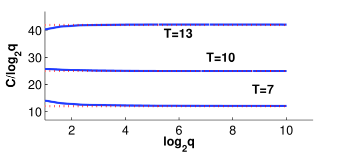
Figure 1: Numerical calculation of the capacity for small values of $q$ and $m=11$, $n=7$. The dotted line depicts $i^{*}(T-i^{*})$.

From Theorem 3, we can derive the following guidelines for non-coherent network code design.

III-A1 Choice of subspaces

The optimal input distribution uses subspaces of a single dimension equal to $\min[m,n]$ for $T\geq\min[m,n]+n$. As $T$ reduces, the set of used subspaces gradually increases, by activating one by one smaller and smaller dimensional subspaces, until, for $T\leq n$, all subspaces are used with equal probability. Fig. 2 pictorially depicts this gradual inclusion of subspaces.

This behavior is different from the result of [16] where all the subspaces up to dimension equal to the min-cut appeared in the optimal input distribution. This difference is due to the different channel model used in our work and in [16].

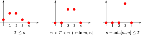
Figure 2: Probability mass function of the active subspace dimensions for channel parameters $m=4$, $n=3$. As it is shown in Theorem 3 there exist three different regimes.

III-A2 Values of m and n

For a given and fixed packet length $T$, the optimal value of $m$ and $n$ equals $m=n=\lfloor T/2\rfloor$ (optimality is in the sense of minimum requirement in order to obtain the maximum capacity for this $T$). For fixed $T$ and $m$, the optimal value of $n$ equals $n=\min[m,\lfloor T/2\rfloor]$. For fixed $T$ and $n$, the optimal value of $m$ equals $m=\min[n,\lfloor T/2\rfloor]$.

TABLE I: Information loss from using coding vectors when $n=m$.

	$T\leq 2m$	$T>2m$
$C_{\textsl{m}}-R_{\textsl{cv}}$	$o(1)$	$o(1)=(i^{*}-1)(T-i^{*})\frac{\log_{2}{q}}{q}+O(q^{-1})$

III-A3 Subspace coding vs. coding vectors

One of the aims of this work was to find the regimes in which the using of coding vectors [12] is far from optimal. Table I summarizes this difference. As we see from the Table I subspace coding does not offer benefits as compared to the coding vectors approach for large field size.

Table I is calculated as follows. The achievable rate $R_{\textsl{cv}}$ using coding vectors equals

$$R_{\textsl{cv}}\triangleq{\mathbb{P}\left[\mathrm{rank}(G_{k})=k\right]}k(T-k)\log_{2}{q},$$

where $0<k\leq m$ is the number of packets in each generation, i.e., each packet includes a coding vector of length $k$ and $T-k$ information symbols. Equivalently, we assume that we use $k$ of the $m$ possible input packets. The matrix $G_{k}$ is the $k\times k$ sub-matrix of $G$ that is applied over the input packets. To calculate $R_{\textsl{cv}}$, we know that ${\mathbb{P}\left[\mathrm{rank}(G_{k})=k\right]}=\prod_{i=0}^{k-1}(1-q^{-k+i})=1-q^{-1}+O(q^{-2})$. Assume we choose $k=i^{*}$ we have $R_{\textsl{cv}}=i^{*}(T-i^{*})\log_{2}{q}-i^{*}(T-i^{*})\frac{\log_{2}{q}}{q}$, where $i^{*}=\min\left[m,n,\lfloor T/2\rfloor\right]$. For the capacity $C_{\textsl{m}}$ we use the large $q$-regime as considered in Theorem 2 for the case $T\leq 2m$ and the finite $q$-regime of Theorem 4 for the case $T>2m$.

III-B Extension to the packet erasure networks

After the error free single source scenario, we consider packet erasure networks, and calculate an upper and lower bound on the capacity for this case. The work in [16], which is the closest to ours, did not consider erasures but instead constant-dimension additive errors. In practice, depending on the application, either of the models might be more suitable: for example, if network coding is deployed at an application layer, then, unless there exist malicious attackers, packet erasures are typically used to abstract both the underlying physical channel errors, as well as packet dropped at queues or lost due to expired timers.

We model the erasures in the network as an end-to-end phenomenon which randomly erases packets according to some probability distribution. Formally, we rewrite the channel defined in (4) as

$$Y[t]=E[t]G[t]X[t],$$ (15)

where $G\in\mathbb{F}_{q}^{m\times m}$ is assumed to be a squre chanel matrix and $E\in\mathbb{F}_{q}^{m\times m}$ is a diagonal random matrix whose elements on its diagonal are either $1$ or $0$. We also assume that $q$ is large, and as a result the transfer matrix is full rank with high probability. Moreover, we consider the case where $m\leq\frac{T}{2}$, i.e. the matrix $X$ is a fat matrix. Recall that we can think of the rows of this matrix as packets send by the source, and the rows of the $Y$ matrix as packets received at the destination.

Note that in equation (15) all of the erasure events are captured by the erasure matrix $E[t]$. Moreover, the erasure pattern is important only up to determining the number of packets that the destination receives, since the transfer matrix $G[t]$ is unknown and distributed uniformly at random over all full rank matrices. Thus, we model the number of received packets (number of non-zero elements on the diagonal of $E[t]$) as a random variable $N$ which takes values in $0\leq N\leq m$ according to some distribution that depends on the packet erasures in the network. In this case the capacity is

$$C_{e}=\max_{P_{X}}I(X;Y,N).$$

We can then use our previous result, Theorem 2, to find an upper and lower bound for the capacity $C_{e}$ when we have packet erasure in the network, as the following Theorem 5 describes.

Theorem 5

Let the number of received packets at the destination be a random variable $N$ defined over the set of integers $0\leq N\leq m$. Also, assume that $m\leq T/2$. Then for large $q$, we have the following upper and lower bound for the capacity $C_{e}$,

$$\mu_{1}(T-m)\log_{2}{q}\leq C_{e}\leq\mu_{1}\left(T-\frac{\mu_{2}}{\mu_{1}}\right)\log_{2}{q},$$

where $\mu_{1}\triangleq{\mathbb{E}_{N}\left[N\right]}$ and $\mu_{2}\triangleq{\mathbb{E}_{N}\left[N^{2}\right]}$.

For the proof of Theorem 5 and more discussion refer to Appendix B.

Note that because we do not necessarily employ full-rank matrices $X$, it is possible that although some packets are erased at the destination, the received packets still span a matrix of the same rank as $X$; thus erasing packets is not equivalent to erasing dimensions.

III-C Multiple Sources

In several practical applications, such as sensor networks, data sources are not necessarily co-located. We thus extend our work to the case where multiple not co-located sources transmit information to a common receiver. In particular, we consider the non-coherent MAC introduced in Definition 6, and characterize the capacity region of this network for the case of two sources with $m_{1}$ and $m_{2}$ input packets and packet length $T>2(m_{1}+m_{2})$. We believe that this technique can be extended to more than two sources.

To find the rate region of the matrix multiple access channel $\mathrm{Ch}_{\textsl{m-MAC}}$, we first show that the two channels $\mathrm{Ch}_{\textsl{m-MAC}}$ and $\mathrm{Ch}_{\textsl{s-MAC}}$ are equivalent, as stated in Theorem 6. We then find the rate region of the subspace multiple access channel $\mathrm{Ch}_{\textsl{s-MAC}}$ which is stated in Theorem 7. To avoid repetition, we state Theorem 6 without a proof because its proof is very similar to that of Theorem 1.

Theorem 6

The matrix MAC $\mathrm{Ch}_{\textsl{m-MAC}}$ defined in Definition 6 is equivalent to the subspace MAC $\mathrm{Ch}_{\textsl{s-MAC}}$ defined in Definition 7 in the sense that the optimal rate region for these two channels is the same.

Theorem 7

For $\frac{T}{2}>m_{1}+m_{2}$, the asymptotic (in the field size $q$) capacity region of the MAC $\mathrm{Ch}_{\textsl{m-MAC}}$ introduced in Definition 6 is given by

$$\mathcal{R}^{*}\triangleq\mathrm{convex~{}hull}\bigcup_{(d_{1},d_{2})\in\mathcal{D}^{*}}\mathcal{R}(d_{1},d_{2}),$$

where

$$\mathcal{R}(d_{1},d_{2})\triangleq\{(R_{1},R_{2}):R_{i}\leq R_{i}(d_{1},d_{2}),\ i=1,2\},$$ (16)

$$R_{i}(d_{1},d_{2})\triangleq d_{i}(T-d_{1}-d_{2})\log_{2}q,\qquad i=1,2,$$

and

$$\mathcal{D}^{*}\triangleq\{(d_{1},d_{2}):\;\; 0\leq d_{i}\leq\min[n,m_{i}],0\leq d_{1}+d_{2}\leq\min[n,m_{1}+m_{2}]\}.$$

We note that the rate region forms a polytopes that has the following number of corner points (see Corollary 1 in §V)

$$\min\left[m_{1},(n-m_{2})^{+}\right]+\min\left[m_{2},(n-m_{1})^{+}\right]+2-\mathds{1}_{\{n\geq m_{1}+m_{2}\}}.$$

The rate region $\mathcal{R}^{*}$ is shown in Fig. 3 for a particular choice of parameters.

The proof of this theorem is provided in §V. We first derive an outer bound by deriving two other bounds: a cooperative bound and a coloring bound. For the coloring bound, we utilize a combinatorial approach to bound the number of distinguishable symbol pairs that can be transmitted from the sources to the receiver. We then show that a simple scheme that uses coding vectors achieves the outer bound. We thus conclude that, for the case of two sources when $\frac{T}{2}>m_{1}+m_{2}$, use of coding vectors is (asymptotically) optimal.

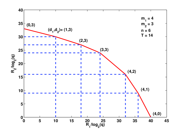
Figure 3: The MAC region $\mathcal{R}^{*}$ for parameters $m_{1}=4$, $m_{2}=3$, $n=3$, $T=14$.

IV The Channel Capacity: Single Source Scenario

In this section we will prove Theorem 2, Theorem 3, and Theorem 4.

IV-A Equivalence of the Matrix Channel $\mathrm{Ch}_{\textsl{m}}$ and the Subspace Channel $\mathrm{Ch}_{\textsl{s}}$

For convenience let us rewrite the channel (4) again

$$Y=GX.$$

To find the capacity of the above channel we need to maximize the mutual information between the input and the output of the channel with respect to the input distribution $P_{X}(x)$. Since the rows of $G$ are chosen independently of each other, assuming that a matrix $X=x$ has been transmitted, we can think of the rows of the received matrix $Y$ as chosen independently from each other, among all the possible vectors in the row span of $x$. The independence of rows of $Y$ allows us to write the conditional probability of $Y$ given $X$, referred to as the channel transition probability, as follows

$$P_{Y|X}(y|x)=\left\{\begin{array}[]{ll}q^{-n\dim(\left\langle x\right\rangle)}&\left\langle y\right\rangle\sqsubseteq\left\langle x\right\rangle,\\ 0&\text{otherwise},\end{array}\right.$$ (17)

where $x\in\mathcal{X}=\mathbb{F}_{q}^{m\times T}$, and $y\in\mathcal{Y}=\mathbb{F}_{q}^{n\times T}$.

The mutual information $I(X;Y)$ between $X$ and $Y$ is a function of $P_{X}(x)$ and $P_{Y|X}(y|x)$ that can be expressed as

$$I(X;Y)=\sum_{\begin{subarray}{l}x\in\mathcal{X},\\ y\in\mathcal{Y}\end{subarray}}P_{X}(x)P_{Y|X}(y|x)\log_{2}\left(\frac{P_{Y|X}(y|x)}{P_{Y}(y)}\right).$$ (18)

It is clear from (17) that $P_{Y|X}(y|x_{1})=P_{Y|X}(y|x_{2})$ for all $x_{1},x_{2}\in\mathcal{X}$ such that $\left\langle x_{1}\right\rangle=\left\langle x_{2}\right\rangle$ which reveals symmetry for the channel $\mathrm{Ch}_{\textsl{m}}$. We exploit this symmetry to show that $C_{\textsl{m}}=C_{\textsl{s}}$ as it is stated in Theorem 1 and proved in Appendix A.

The proof of Theorem 1 determines how we can map an input distribution of $\mathrm{Ch}_{\textsl{s}}$ to an input distribution for $\mathrm{Ch}_{\textsl{m}}$ that achieves the same mutual information. The input distribution $P_{X}(x)$ should be chosen such that we have $\sum_{x\in\mathcal{X}:\left\langle x\right\rangle=\pi_{x}}P_{X}(x)=P_{\Pi_{X}}(\pi_{x})$. One simple way to do this is to put all the probability mass of $\pi_{x}$ on one matrix $x$ such that $\left\langle x\right\rangle=\pi_{x}$.

IV-B Upper and Lower bound for the Capacity of $\mathrm{Ch}_{\textsl{m}}$

Here, we state the proof of Theorem 2 by giving upper and lower bounds for the capacity that differ in $o(1)$ bits, which vanishes as $q\rightarrow\infty$.

Let $C_{\textsl{m}}(n,m,T)$ denote the capacity of the channel $\mathrm{Ch}_{\textsl{m}}$. Let $C_{\textsl{f-m}}(n,m,T)$ denote the capacity of the channel $Y=AX$ where $A\in\mathbb{F}_{q}^{n\times m}$ is a full-rank matrix chosen uniformly at random among all the full-rank matrices in $\mathbb{F}_{q}^{n\times m}$. Then, we have the following lemma.

Lemma 5

We can bound $C_{\textsl{m}}(n,m,T)$ from above and below as follows

$$C_{\textsl{m}}(h,h,T)\leq C_{\textsl{m}}(n,m,T)\leq C_{\textsl{f-m}}(n,m,T)\leq C_{\textsl{f-m}}(h,h,T),$$

where $h=\min[m,n]$.

Proof:

Let $U_{n\times m}\in\mathbb{F}_{q}^{n\times m}$ denote a generic random matrix chosen uniformly at random and independently from any other variable. Similarly, let $A_{n\times m}\in\mathbb{F}_{q}^{n\times m}$ denote a generic full-rank matrix chosen uniformly at random among all such full-rank matrices and independent from any other variable. (Note that each new instance of such a matrix in the same equation denotes a different random variable which is independent from the other random variables.)

Since the channel $Y=A_{n\times m}X$ is statistically equivalent to the channel $Y=A_{n\times n}A_{n\times m}A_{m\times m}X$, we have, by the data processing inequality, that $C_{\textsl{f-m}}(n,m,T)\leq C_{\textsl{f-m}}(h,h,T)$.

Using the same argument, since the channel $Y=U_{n\times m}X$ is equivalent to the channel $Y=U_{n\times n}A_{n\times m}X$ if $n\geq m$, and is equivalent to the channel $Y=A_{n\times m}U_{m\times m}X$ if $n\leq m$ we have $C_{\textsl{m}}(n,m,T)\leq C_{\textsl{f-m}}(n,m,T)$.

To obtain the lower bound we proceed as follows. Let us choose $X=\left[\begin{smallmatrix}I_{h}\\ \\ 0\end{smallmatrix}\right]\overline{X}$ and $\overline{Y}=\left[I_{h}\ \ 0\right]Y$, where $Y=U_{n\times m}X$. Then we can write

$$\overline{Y}=\left[I_{h}\ \ 0\right]U_{n\times m}{I_{h}\brack 0}\overline{X}=U_{h\times h}\overline{X},$$

where $U_{h\times h}$ is the upper left $h\times h$ sub-matirx of $U_{n\times m}$. Thus, again the data processing inequality implies that $C_{\textsl{m}}(h,h,T)\leq C_{\textsl{m}}(n,m,T)$. ∎

Lemma 6

For $C_{\textsl{m}}(n,m,T)$ we have

$$C_{\textsl{m}}(n,m,T)\leq i^{*}(T-i^{*})\log_{2}{q}+o(1),$$

where $i^{*}=\min[m,n,\lfloor T/2\rfloor]$.

Proof:

By Lemma 5 we have

$$C_{\textsl{m}}(n,m,T) \leq C_{\textsl{f-m}}(h,h,T)$$

$$\stackrel{{\scriptstyle(a)}}{{=}}\log_{2}\left(\sum_{i=0}^{h}{T\brack i}\right)$$

$$\stackrel{{\scriptstyle(b)}}{{=}}i^{*}(T-i^{*})\log_{2}{q}+o(1),$$

where $(a)$ follows from [16, Corollary 2] and $(b)$ follows from Lemma 1. ∎

Lemma 7

For $C_{\textsl{m}}(n,m,T)$ we have

$$C_{\textsl{m}}(n,m,T)\geq i^{*}(T-i^{*})\log_{2}{q}-o(1),$$

where $i^{*}=\min[m,n,\lfloor T/2\rfloor]$.

Proof:

For every subspace $\Pi\in\mathrm{Gr}(T,i^{*})$, let $\mathrm{RREF}(\Pi)\in\mathbb{F}_{q}^{i^{*}\times T}$ be a matrix in reduced row echelon form such that $\Pi=\left\langle\mathrm{RREF}(\Pi)\right\rangle$. Choose $X=\left[\begin{smallmatrix}I_{i^{*}}\\ \\ 0\end{smallmatrix}\right]\times\mathrm{RREF}(\Pi_{X})\in\mathbb{F}_{q}^{m\times T}$, where $\Pi_{X}$ is chosen uniformly at random from $\mathrm{Gr}(T,i^{*})$. Define the random variable $Q=\mathds{1}_{\{\mathrm{rank}(Y)=i^{*}\}}$. Note that $\Pi_{Y}=\Pi_{X}$ when $Q=1$. Thus, we have $H(\Pi_{Y}|\Pi_{X},Q=1)=0$ and $H(\Pi_{Y}|Q=1)=H(\Pi_{X})=\log_{2}{T\brack i^{*}}\geq i^{*}(T-i^{*})\log_{2}{q}$. Then, it follows that

$$C_{\textsl{m}}(n,m,T) \stackrel{{\scriptstyle(a)}}{{\geq}}C_{\textsl{m}}(h,h,T)$$

$$\stackrel{{\scriptstyle(b)}}{{\geq}}I(\Pi_{X};\Pi_{Y})$$

$$\stackrel{{\scriptstyle(c)}}{{=}}I(\Pi_{X};\Pi_{Y},Q)$$

$$=I(\Pi_{X};Q)+I(\Pi_{X};\Pi_{Y}|Q)$$

$$\geq{\mathbb{P}\left[Q=1\right]}I(\Pi_{X};\Pi_{Y}|Q=1)$$

$$\geq{\mathbb{P}\left[Q=1\right]}i^{*}(T-i^{*})\log_{2}{q},$$

where $(a)$ is due to Lemma 5, $(b)$ follows follows from Theorem 1, and $(c)$ holds since $Q$ is a deterministic function of $\Pi_{Y}$. Now, note that we can write

$${\mathbb{P}\left[Q=1\right]} ={\mathbb{P}\left[\mathrm{rank}(U_{h\times h}X)=i^{*}\right]}$$

$$={\mathbb{P}\left[\mathrm{rank}\left(U_{h\times h}\left[\begin{smallmatrix}I_{i^{*}}\\ \\ 0\end{smallmatrix}\right]\right)=i^{*}\right]}$$

$$={\mathbb{P}\left[\mathrm{rank}(U_{h\times i^{*}})=i^{*}\right]}$$

$$\geq 1-\frac{i^{*}}{q^{k-i^{*}+1}}$$

$$\geq 1-\frac{i^{*}}{q},$$

and thus we obtain the desired result. ∎

Combining Lemma 6 and Lemma 7 recovers Theorem 2.

IV-C The Optimal Solution: General Approach

Generally, we are interested in finding the capacity and input distribution of $\mathrm{Ch}_{\textsl{m}}$ exactly. It is shown in Theorem 1 that instead of the channel $\mathrm{Ch}_{\textsl{m}}$ we can focus on the channel $\mathrm{Ch}_{\textsl{s}}$. Thus, we are interested in optimizing the following quantity

$$I(\Pi_{X};\Pi_{Y})=\sum_{\begin{subarray}{l}\pi_{x}\in\widetilde{\mathcal{X}},\\ \pi_{y}\in\widetilde{\mathcal{Y}}\end{subarray}}P_{\Pi_{X}}(\pi_{x})P_{\Pi_{Y}|\Pi_{X}}(\pi_{y}|\pi_{x})\log_{2}\left(\frac{P_{\Pi_{Y}|\Pi_{X}}(\pi_{y}|\pi_{x})}{P_{\Pi_{Y}}(\pi_{y})}\right).$$ (19)

Remember that $\widetilde{\mathcal{X}}=\mathrm{Sp}(T,m)$ and $\widetilde{\mathcal{Y}}=\mathrm{Sp}(T,n)$.

The following lemma states that the optimal solution for the channel $\mathrm{Ch}_{\textsl{s}}$ should be uniform over all subspaces with the same dimension, as it is intuitively expected from the symmetry of the channel.

Lemma 8

The input distribution that maximizes $I(\Pi_{X};\Pi_{Y})$ for $\mathrm{Ch}_{\textsl{s}}$ is the one which is uniform over all subspaces having the same dimension.

Lemma 8 shows that the optimal input distribution can be expressed as

$${\mathbb{P}\left[\Pi_{X}=\pi_{x}\right]}=\frac{\alpha_{d_{x}}}{{T\brack d_{x}}},$$ (20)

where $d_{x}=\dim(\pi_{x})$, $\alpha_{d_{x}}={\mathbb{P}\left[\dim(\Pi_{X})=d_{x}\right]}$, and we have $\sum_{d_{x}=0}^{\min[m,T]}\alpha_{d_{x}}=1$. We can then simplify $I(\Pi_{X};\Pi_{Y})$ as stated in the following lemma.

Lemma 9

Assuming an optimal input probability distribution of the form in (20), the mutual information $I(\Pi_{X};\Pi_{Y})$ can be simplified to

$$I(\Pi_{X};\Pi_{Y})= -\sum_{d_{x}=0}^{\min[m,T]}\alpha_{d_{x}}nd_{x}\log_{2}{q}$$

$$-\sum_{d_{x}=0}^{\min[m,T]}\alpha_{d_{x}}q^{-nd_{x}}\sum_{d_{y}=0}^{\min[n,d_{x}]}\psi(n,d_{y}){d_{x}\brack d_{y}}\log_{2}(f(d_{y})),$$ (21)

where

$$f(d_{y})\triangleq\frac{P_{\Pi_{Y}}(\pi_{y})}{\psi(n,d_{y})}=\frac{1}{{T\brack d_{y}}}\sum_{d_{x}=d_{y}}^{\min[m,T]}{d_{x}\brack d_{y}}q^{-nd_{x}}\alpha_{d_{x}}.$$ (22)

Lemmas 8 and 9 show that the problem of finding the optimal input distribution for the channel $\mathrm{Ch}_{\textsl{s}}$ is reduced to finding the optimal choice for $\alpha_{i},\ i=0,\dots,\min[m,T]$. We know that the mutual information is a concave function with respect to $P_{\Pi_{X}}(\pi_{x})$’s. Observation 1 implies that because (20) is a linear transformation from $P_{\Pi_{X}}(\pi_{x})$’s to $\alpha_{i}$’s, as a result the mutual information $I(\Pi_{X};\Pi_{Y})$ is also concave with respect to $\alpha_{i}$’s [18].

Observation 1

Let $g(\mathbf{x})$ be a concave function and let $\mathbf{x}=h(\mathbf{z})$ be a linear transform from $\mathbf{z}$ to $\mathbf{x}$. Then $g(h(\mathbf{z}))$ is also a concave function.

Using Observation 1, we know that the mutual information is a concave function with respect to $\alpha_{i}$’s. This allows us to use the Kuhn-Tucker theorem [18] to solve the convex optimization problem. According to this theorem, the set of probabilities $\alpha_{i}^{*}$, $0\leq i\leq\min[m,T]$, maximize the mutual information if and only if there exists some constant $\lambda$ such that

$$\left\{\begin{array}[]{ll}\left.\frac{\partial I(\Pi_{X};\Pi_{Y})}{\partial\alpha_{k}}\right|_{\boldsymbol{\alpha}^{*}}=\lambda&\forall k:\ \alpha^{*}_{k}>0,\\ \\ \left.\frac{\partial I(\Pi_{X};\Pi_{Y})}{\partial\alpha_{k}}\right|_{\boldsymbol{\alpha}^{*}}\leq\lambda&\forall k:\ \alpha^{*}_{k}=0,\end{array}\right.$$ (23)

where $\sum_{i=0}^{\min[m,T]}\alpha^{*}_{i}=1$, $0\leq k\leq\min[m,T]$, and $\boldsymbol{\alpha}^{*}$ is the vector of the optimum input probabilities of choosing subspaces of certain dimension,

$$\boldsymbol{\alpha}^{*}=\left[\begin{array}[]{ccc}\alpha^{*}_{0}&\cdots&\alpha^{*}_{\min[m,T]}\end{array}\right]^{\mathrm{T}}.$$

Lemma 10

By taking the partial derivative of the mutual information given in (9) with respect to $\alpha_{k}$, we have

$$I^{\prime}_{k}\triangleq\frac{\partial I(\Pi_{X};\Pi_{Y})}{\partial\alpha_{k}}=-nk\log_{2}{q}-\sum_{d_{y}=0}^{\min[n,k]}\psi(n,d_{y}){k\brack d_{y}}q^{-nk}\log_{2}\left(f(d_{y})\right)-\log_{2}{e}.$$ (24)

Multiplying both sides of (24) by $\alpha_{k}$ and summing over $k$ we get

$$I-\log_{2}{e}=\sum_{k=0}^{\min[m,T]}\alpha_{k}I^{\prime}_{k}.$$

By choosing the optimal values $\alpha_{k}=\alpha^{*}_{k}$ for $0\leq k\leq\min[m,T]$, the RHS becomes $\lambda$, and the mutual information increases to $C_{\textsl{s}}$. So we may write $\lambda=C_{\textsl{s}}-\log_{2}{e}$.

IV-D Solution for Large Field Size

In this subsection, we focus on large size fields, $q\gg 1$. This assumption allows us to use some approximations to simplify the conditions in (23). Assuming large $q$ we can rewrite (24) as follows

$$I^{\prime}_{k}=-nk\log_{2}{q}-\log_{2}{e}-\sum_{d_{y}=0}^{\min[n,k]}\left(1+O(q^{-1})\right)q^{-(n-d_{y})(k-d_{y})}\log_{2}\left(f(d_{y})\right),$$ (25)

where we have used Lemma 1 and Lemma 3. Using similar approximations, $\log_{2}f(d_{y})$ defined in (22) can be approximated as

$$\log_{2}\left(f(d_{y})\right)= -d_{y}T\log_{2}{q}+O(q^{-1})+\log_{2}\left(\sum_{d_{x}=d_{y}}^{\min[m,T]}q^{-(n-d_{y})d_{x}}\alpha_{d_{x}}\right).$$ (26)

Then we have the following result, Lemma 11.

Lemma 11

The dominating term in the summation in (25) is the one obtained for $d_{y}=\min[n,k]$.

From the proof of Lemma 11 written in Appendix A, we can also see that the remaining terms in the summation of (25) are of order $o(1)$, so we can write

$$I^{\prime}_{k}= [T\min[n,k]-nk]\log_{2}{q}+\underbrace{o(1)}_{\epsilon_{q}(k)}-\log_{2}{e}-\log_{2}\left(\sum_{d_{x}=\min[n,k]}^{\min[m,T]}q^{-[n-\min[n,k]]d_{x}}\alpha_{d_{x}}\right).$$ (27)

Assuming that the expression inside the $\log(\cdot)$ function in (27) is not zero for every $0\leq k\leq\min[m,T]$, we can rewrite the Kuhn-Tucker conditions as

$$\sum_{d_{x}=\min[n,k]}^{\min[m,T]}q^{-[n-\min[n,k]]d_{x}}\alpha_{d_{x}}\geq 2^{-C_{\textsl{s}}+o(1)}q^{[T\min[n,k]-nk]},$$

where the inequality holds with equality for all $k$ with $\alpha_{k}^{*}>0$.

Let $\delta\triangleq\min[m,T]$ and define the $(\delta+1)\times(\delta+1)$ matrix $\mathbf{A}$ with elements

$$\mathbf{A}_{ij}\triangleq\left\{\begin{array}[]{ll}q^{-[n-\min[n,i]]j}&\min[n,i]\leq j\leq\delta,\\ 0&\textrm{otherwise}.\end{array}\right.$$

We also define the column vector $\mathbf{b}$ with elements $\mathbf{b}_{i}\triangleq q^{[T\min[n,i]-ni]}$ for $0\leq i\leq\delta$. Note that for convenience the indices of matrix $\mathbf{A}$ and vector $\mathbf{b}$ start from $0$. Using these definitions, we are able to rewrite the Kuhn-Tucker conditions in the matrix form as

$$\mathbf{A}\boldsymbol{\alpha}^{*}\succeq 2^{-C_{\textsl{s}}+o(1)}\mathbf{b}.$$ (28)

In the following, we consider two cases for $\delta\leq n$ and $\delta>n$, and find $\boldsymbol{\alpha}^{*}$ for each of them, separately.

First case: $\delta\leq n$. In this case we can explicitly write the matrix $\mathbf{A}$ and vector $\mathbf{b}$ as

$$\mathbf{A}=\left[\begin{array}[]{cccccc}1&q^{-n}&\cdots&q^{-(\delta-1)n}&q^{-\delta n}\\ 0&q^{-(n-1)}&\cdots&q^{-(\delta-1)(n-1)}&q^{-\delta(n-1)}\\ 0&0&\cdots&q^{-(\delta-1)(n-2)}&q^{-\delta(n-2)}\\ \vdots&\vdots&\ddots&\vdots&\vdots\\ 0&0&\cdots&q^{-(\delta-1)(n-\delta+1)}&q^{-\delta(n-\delta+1)}\\ 0&0&\cdots&0&q^{-\delta(n-\delta)}\end{array}\right],$$

and

$$\mathbf{b}=\left[\begin{array}[]{cccc}1&q^{(T-n)}&\cdots&q^{\delta(T-n)}\end{array}\right]^{\mathrm{T}}.$$

The fact that the expression inside the $\log_{2}(\cdot)$ function in (27) is non-zero for $k=\delta$, forces $\alpha_{\delta}^{*}$ to be positive. Thus the last row of the matrix inequality in (28) should be satisfied as an equality. Therefore,

$$\alpha^{*}_{\delta}= \frac{q^{\delta(T-n)}}{q^{-\delta(n-\delta)}}2^{-C_{\textsl{s}}+o(1)}=q^{\delta(T-\delta)}2^{-C_{\textsl{s}}+o(1)}.$$

Now we use induction to show that the optimal solution has the form

$$\alpha^{*}_{i}=\left\{\begin{array}[]{lcl}q^{i(T-i)}2^{-C_{\textsl{s}}+o(1)}&:&\kappa\leq i\leq\delta,\\ 0&:&0\leq i<\kappa,\end{array}\right.$$ (29)

where we will determine $\kappa$ later.

Let us fix $l$ and assume that $\alpha^{*}_{i}=q^{i(T-i)}2^{-C_{\textsl{s}}+o(1)}$ for $0\leq l<i\leq\delta$. Then for $\alpha^{*}_{l}$ we can write

$$A_{ll}\alpha^{*}_{l}+\sum_{j=l+1}^{\delta}q^{-(n-l)j}\alpha^{*}_{j}\geq q^{l(T-n)}2^{-C_{\textsl{s}}+o(1)},$$

or equivalently

$$A_{ll}\alpha^{*}_{l}\geq q^{l(T-n)}2^{-C_{\textsl{s}}+o(1)}-\sum_{j=l+1}^{\delta}q^{-(n-l)j}\alpha^{*}_{j}$$

$$= q^{l(T-n)}2^{-C_{\textsl{s}}+o(1)}\left[1-\sum_{j=l+1}^{\delta}q^{(T-n-j)(j-l)}\right].$$ (30)

We can use induction for one step more to show that $\alpha^{*}_{l}$ is of the desired form (29) if the previous expression is satisfied with equality. This is true if we have $1-\sum_{j=l+1}^{\delta}q^{(T-n-j)(j-l)}\geq 0$, or equivalently (assuming large $q$) if we have $\left.(T-n-j)\right|_{j=l+1}<0$. So we can conclude that we should have $(T-n)^{+}\leq l\leq\delta$. It can be easily verified that for $i<(T-n)^{+}$ the Kuhn-Tucker equation for $\alpha^{*}_{i}$ satisfies the strict inequality so $\alpha^{*}_{i}=0$ for $i<\min[(T-n)^{+},\delta]$. The above argument results in a solution of the following form for the case $\delta\leq n$

$$\alpha^{*}_{i}=\left\{\begin{array}[]{lcl}q^{i(T-i)}2^{-C_{\textsl{s}}+o(1)}&:&\min\left[(T-n)^{+},\delta\right]\leq i\leq\delta,\\ 0&:&0\leq i<\min\left[(T-n)^{+},\delta\right].\end{array}\right.$$ (31)

Second case: $\delta>n$. We now write matrix $\mathbf{A}$ and vector $\mathbf{b}$ as

$$\mathbf{A} =\left[\begin{matrix}1&q^{-n}&\cdots&\cdots&\cdots&\cdots&q^{-\delta n}\\ 0&q^{-(n-1)}&\cdots&\cdots&\cdots&\cdots&q^{-\delta(n-1)}\\ \vdots&\ddots&\ddots&\vdots&\vdots&\vdots&\vdots\\ 0&\cdots&0&q^{-(n-1)}&q^{-n}&\cdots&q^{-\delta}\\ \hline\cr 0&\cdots&0&0&1&\cdots&1\\ \vdots&\ddots&\vdots&\vdots&\vdots&\ddots&\vdots\\ 0&\cdots&0&0&1&\cdots&1\\ \end{matrix}\right],$$

and

$$\mathbf{b}=\left[\begin{matrix}1&q^{(T-n)}&\cdots&q^{(n-1)(T-n)}&q^{n(T-n)}&q^{n(T-n-1)}&\cdots&q^{n(T-\delta)}\end{matrix}\right]^{\mathrm{T}}.$$

The last $\delta-n+1$ rows of $\mathbf{A}$ are the same while $b_{i}$ is decreasing with $i$ for $i\geq n$. Thus, the last $\delta-n$ inequalities are strict and therefore,

$$\alpha^{*}_{n+1}=\cdots=\alpha^{*}_{\delta}=0.$$ (32)

The remaining equations can simply be reduced to the first case. Define

$$\tilde{\mathbf{A}}=\left[\begin{array}[]{cccccc}1&q^{-n}&\cdots&q^{-(n-1)n}&q^{-n^{2}}\\ 0&q^{-(n-1)}&\cdots&q^{-(n-1)(n-1)}&q^{-n(n-1)}\\ 0&0&\cdots&q^{-(n-1)(n-2)}&q^{-n(n-2)}\\ \vdots&\vdots&\ddots&\vdots&\vdots\\ 0&0&\cdots&q^{-(n-1)}&q^{-n}\\ 0&0&\cdots&0&1\end{array}\right],$$

and

$$\tilde{\mathbf{b}}=\left[\begin{array}[]{cccc}1&q^{(T-n)}&\cdots&q^{n(T-n)}\end{array}\right]^{\mathrm{T}}.$$

The remaining conditions in this case can be written as

$$\tilde{\mathbf{A}}\boldsymbol{\alpha}^{*}\succeq 2^{-C_{\textsl{s}}+o(1)}\tilde{\mathbf{b}},$$

which is exactly similar to (28), for $\delta=n$. Therefore, the optimal solution for the first case will also satisfy these conditions, i.e.,

$$\alpha^{*}_{i}=\left\{\begin{array}[]{ll}q^{i(T-i)}2^{-C_{\textsl{s}}+o(1)}&\kappa\leq i\leq n,\\ 0&0\leq i<\kappa,\end{array}\right.$$ (33)

with $\kappa=\min[(T-n)^{+},n]$. Summarizing (32) and (33), we can obtain the optimal solution for this regime, as

$$\alpha^{*}_{i}=\left\{\begin{array}[]{ll}0&n<i\leq\delta,\\ q^{i(T-i)}2^{-C_{\textsl{s}}+o(1)}&\kappa\leq i\leq n,\\ 0&0\leq i<\kappa,\end{array}\right.$$ (34)

where $\kappa=\min[(T-n)^{+},n]$. This completes the proof of Theorem 3. By normalizing $\alpha^{*}_{i}$ to $1$ we can also obtain an alternative proof to Theorem 2.

Discussion: To characterize the exact value of $q_{0}$ one have to consider the exact form of the set of equations given in (IV-D) (for each $l$) which are as follows,

$$A_{ll}\alpha^{*}_{l}\geq q^{l(T-n)}2^{-C_{\textsl{s}}+\epsilon_{q}(l)}\left[1-\sum_{j=l+1}^{\delta}q^{(T-n-j)(j-l)}2^{[\epsilon_{q}(j)-\epsilon_{q}(l)]}\right].$$

Although it is hard to find $q_{0}$ exactly, it is possible to show that there exists finite $q_{0}$ such that result of Theorem 3 holds for. This can be done by solving above equations assuming that $\epsilon_{q}(k)$ is zero for every $k$ (assuming $q\gg 1$). Then, it can be observed that the RHS of (IV-D) are either greater or less than zero. Now by assuming finite but large enough $q$ and considering the exact form of (IV-D) we have some small perturbations that cannot change the sign of RHS of (IV-D) so we are done.

IV-E Proof of Theorem 4

Let $\epsilon_{q}(k)$ denotes the error term in (27). We can easily write the exact expression for $\epsilon_{q}(k)$ which is as follows

$$\epsilon_{q}(k)= -\sum_{d_{y}=0}^{r_{k}}\psi(n,d_{y}){k\brack d_{y}}q^{-nk}\log_{2}\left(\sum_{d_{x}=d_{y}}^{\min[m,T]}\alpha_{d_{x}}\frac{{d_{x}\brack d_{y}}}{{T\brack d_{y}}}q^{-nd_{x}}\right)$$

$$+\log_{2}\left(\sum_{d_{x}=r_{k}}^{\min[m,T]}q^{r_{k}(d_{x}-r_{k})-nd_{x}}\alpha_{d_{x}}\right)-r_{k}(T-r_{k})\log_{2}{q},$$

where $r_{k}=\min[n,k]$.

We consider the case where $T>n+\min[m,n]$ so Theorem 3 implies that for the optimal input distribution we have $\alpha_{i^{*}}=1$ where $i^{*}=\min[m,n]$ and $q>q_{0}$. Then we can simplify $\epsilon_{q}(k)$ more and write

$$\epsilon_{q}(k)= \sum_{d_{y}=0}^{r_{k}}\psi(n,d_{y}){k\brack d_{y}}q^{-nk}\log_{2}\left(\frac{{T\brack d_{y}}}{{i^{*}\brack d_{y}}}\right)-r_{k}(T-i^{*}),$$ (35)

where we also use Lemma 4 in the above simplification.

To find $q_{0}$, the minimum value of $q$ that the result of Theorem 4 is valid for, we should consider the exact form of (IV-D) and check that the RHS of (IV-D) is less than or equal to zero for $0\leq l\leq(i^{*}-1)$. So from (IV-D) for every $0\leq l\leq(i^{*}-1)$ we may write

$$\left[1-q^{(T-n-i^{*})(i^{*}-l)}2^{\left[\epsilon_{q}(i^{*})-\epsilon_{q}(l)\right]}\right]\leq 0,$$

or equivalently

$$\frac{\epsilon_{q_{0}}(l)-\epsilon_{q_{0}}(i^{*})}{(T-n-i^{*})(i^{*}-l)}\leq\log_{2}{q_{0}},\quad\forall l:0\leq l\leq(i^{*}-1).$$ (36)

Using a similar argument we should have also

$$\frac{\epsilon_{q_{0}}(l)-\epsilon_{q_{0}}(i^{*})}{i^{*}(l-i^{*})}\leq\log_{2}{q_{0}},\quad\forall l:(i^{*}+1)\leq l\leq m.$$ (37)

From (34) for the capacity $C_{\textsl{s}}$ we have $C_{\textsl{s}}=i^{*}(T-i^{*})\log_{2}{q}+\epsilon_{q}(i^{*})$. Evaluating (35) at $k=i^{*}$ we have

$$\epsilon_{q}(i^{*})= \sum_{d_{y}=0}^{i^{*}}\psi(n,d_{y}){i^{*}\brack d_{y}}q^{-ni^{*}}\log_{2}\left(\frac{{T\brack d_{y}}}{{i^{*}\brack d_{y}}}\right)-i^{*}(T-i^{*})\log_{2}{q},$$

which results in the capacity stated in the assertion of Theorem 4.

Discussion: We derive a sufficient condition on the minimum size of $q$ to satisfy the set of conditions stated in (36) and (37). Using this sufficient condition we explore the behavior of $q_{0}$ as $T$ increases.

For $k\neq i^{*}$ we can write

$$\epsilon_{q}(k) \stackrel{{\scriptstyle(a)}}{{\leq}}4\sum_{d_{y}=0}^{r_{k}}q^{-(n-d_{y})(k-d_{y})}\log_{2}\left(4q^{d_{y}(T-i^{*})}\right)-r_{k}(T-i^{*})\log_{2}{q}$$

$$\leq 8+4r_{k}q^{-(\max[n,k]-\min[n,k]+1)}\left(2+(r_{k}-1)(T-i^{*})\log_{2}{q}\right)$$

$$\stackrel{{\scriptstyle(b)}}{{\leq}}(8+8r_{k})+\left(4r_{k}(r_{k}-1)(T-i^{*})\frac{\log_{2}{q}}{q^{(\max[n,k]-\min[n,k]+1)}}\right),$$ (38)

where $(a)$ follows from (2) and (3), and in $(b)$ we use the fact that $k\neq i^{*}$.

Then for $k=i^{*}$ we can write

$$\epsilon_{q}(i^{*}) \geq\psi(n,i^{*})q^{-ni^{*}}\log_{2}{{T\brack i^{*}}}-i^{*}(T-i^{*})\log_{2}{q}$$

$$\stackrel{{\scriptstyle(a)}}{{\geq}}-(i^{*})^{2}(T-i^{*})\frac{\log_{2}{q}}{q^{n-i^{*}+1}},$$ (39)

where $(a)$ follows from (2) and (3).

Let us consider two cases. First, we assume that $m\leq n$ so $i^{*}=m$. To find a sufficient condition for $q_{0}$ we have to only consider conditions given in (36). Using (IV-E) and (IV-E) and assuming that $T\rightarrow\infty$ we should have $\log_{2}{q_{0}}\geq 5m^{2}q_{0}^{-n+m-1}\log_{2}{q_{0}}$, or equivalently $q_{0}^{n-m+1}\geq 5(i^{*})^{2}$.

For the second case we have $m>n$ which means $i^{*}=n$. Here, using a similar argument to the one given above for the first case we can show that conditions (36) give some constant $q_{0}$ as $T\rightarrow\infty$. However, the conditions (37) give a sufficient condition for $q_{0}$ which grows as $T\rightarrow\infty$. Now, using (37), (IV-E), and (IV-E) and assuming that $T\rightarrow\infty$, a sufficient condition for $q_{0}$ would be $\log_{2}{q_{0}}\geq 4nTq_{0}^{-2}\log_{2}{q_{0}}+nTq_{0}^{-1}\log_{2}{q_{0}}$. For large $T$ for the sufficient condition we have $q_{0}\geq i^{*}T$.

V Multiple Sources Scenario: The Rate Region

The goal of this section is to characterize $\mathcal{R}$, the set of all achievable rate pairs $(R_{1},R_{2})$ for two user communication over the multiple access channel $\mathcal{C}_{\textsl{m-MAC}}$ described in Definition 6. More precisely, we will show that $\mathcal{R}=\mathcal{R}^{*}$. In order to do this, we first formulate a mathematical model for this channel. Then, we present an achievability scheme, to show that $\mathcal{R}^{*}$ is achievable, i.e., $\mathcal{R}^{*}\subseteq\mathcal{R}$. In the next subsection we prove the optimality of this scheme and show that $\mathcal{R}\subseteq\mathcal{R}^{*}$.

The proof of the converse part of the theorem is based on two outer bounds, namely, a cooperative bound and a coloring bound. For the coloring bound, we utilize a combinatorial argument to bound the number of distinguishable symbol pairs that can be transmitted from the two sources to the destination. This bound allows us to restrict the effective input alphabets of the sources to subsets of the original alphabets, with significantly smaller size. We can then easily bound the capacity region of the network using the restricted input alphabet.

The transition probability of the channel given by Definition 6, $P_{Y|X_{1}X_{2}}$, can be written as [9]

$$P_{Y|X_{1}X_{2}}(y|x_{1},x_{2})=\left\{\begin{array}[]{ll}q^{-n\dim(\left\langle x_{1}\right\rangle+\left\langle x_{2}\right\rangle)}&\left\langle y\right\rangle\sqsubseteq\left\langle x_{1}\right\rangle+\left\langle x_{2}\right\rangle,\\ 0&\text{otherwise}.\end{array}\right.$$ (42)

Our first result, stated in Theorem 6, is that the multiple access matrix channel described in Definition 6 is equivalent to the “subspace” channel $\mathrm{Ch}_{\textsl{s-MAC}}$ described in Definition 7, that has subspaces as inputs and outputs. So to characterize the optimal rate region of $\mathrm{Ch}_{\textsl{m-MAC}}$, we can focus on finding the optimal rate region of $\mathrm{Ch}_{\textsl{s-MAC}}$. We will use this equivalence in the rest of this section.

We know from [15] that the rate region of the multiple access channel $\mathrm{Ch}_{\textsl{s-MAC}}$ is given by the closure of the convex hull of the rate vectors satisfying

$$R_{S}\leq I(\Pi_{X_{S}};\Pi_{Y}|\Pi_{X_{S^{c}}})\quad\text{for all }S\subseteq\{1,\ldots,N_{s}\},$$

for some product distribution $P_{\Pi_{X_{1}}}(\pi_{1})\cdots P_{\Pi_{X_{N_{s}}}}(\pi_{N_{s}})$. Note that $R_{S}=\sum_{i\in S}R_{i}$, where $R_{i}$ is the transmission rate of the $i$th source, $\Pi_{X_{S}}=\{\Pi_{X_{i}}:i\in S\}$ and $S^{c}$ is the complement set of $S$.

V-A Achievability Scheme

In this subsection we illustrate a simple achievability scheme for the corner points of the rate region defined in Theorem 7. The remaining points in the rate region can be achieved using time-sharing.

For given $(d_{1},d_{2})\in\mathcal{D}^{*}$, define the following subspace code-books

$$\widetilde{\mathcal{C}}_{1}\triangleq\bigg{\{}\left\langle X_{1}\right\rangle:X_{1}=\left[\begin{array}[]{c|c|c}\mathbf{I}_{d_{1}\times d_{1}}&\mathbf{0}_{d_{1}\times d_{2}}&\mathbf{U}_{1}\\ \hline\cr\mathbf{0}_{(m_{1}-d_{1})\times d_{1}}&\mathbf{0}_{(m_{1}-d_{1})\times d_{2}}&\mathbf{0}_{(m_{1}-d_{1})\times(T-d_{1}-d_{2})}\end{array}\right],\mathbf{U}_{1}\in\mathbb{F}_{q}^{d_{1}\times(T-d_{1}-d_{2})}\bigg{\}}$$

and

$$\widetilde{\mathcal{C}}_{2}\triangleq\bigg{\{}\left\langle X_{2}\right\rangle:X_{2}=\left[\begin{array}[]{c|c|c}\mathbf{0}_{d_{2}\times d_{1}}&\mathbf{I}_{d_{2}\times d_{2}}&\mathbf{U}_{2}\\ \hline\cr\mathbf{0}_{(m_{2}-d_{2})\times d_{1}}&\mathbf{0}_{(m_{2}-d_{2})\times d_{2}}&\mathbf{0}_{(m_{2}-d_{2})\times(T-d_{1}-d_{2})}\end{array}\right],\mathbf{U}_{2}\in\mathbb{F}_{q}^{d_{2}\times(T-d_{1}-d_{2})}\bigg{\}}.$$

If we transmit messages from these code-books, we have

$$Y =H_{1}X_{1}+H_{2}X_{2}$$

$$=\left[\begin{array}[]{c|c|c}\hat{H}_{1}&\hat{H}_{2}&\hat{H}_{1}\mathbf{U}_{1}+\hat{H}_{2}\mathbf{U}_{2}\end{array}\right],$$

where $\hat{H}_{i}$ captures the first $d_{i}$ columns of $H_{i}$. Therefore, decoding at the receiver would be just recovering of $\mathbf{U}_{1}$ and $\mathbf{U}_{2}$ given $\hat{H}_{1}\mathbf{U}_{1}+\hat{H}_{2}\mathbf{U}_{2}$, $\hat{H}_{1}$, and $\hat{H}_{2}$. Since $d_{1}+d_{2}\leq n$, the matrix $[\hat{H}_{1}\ \hat{H}_{2}]$ is full-rank with high probability, and therefore the decoder is able to decode $\mathbf{U}_{1}$ and $\mathbf{U}_{2}$.

Note that the achievability scheme uses effectively the coding vectors approach [12]. This indicates that for $\frac{T}{2}>\max[m_{1}+m_{2},n]$ and $q$ large enough, the subspace coding and the coding vectors approach achieve the same rate.

V-B Outer bound on the Admissible Rate Region

In the following we will present an outer bound for $\mathcal{R}$, the admissible rate region of the non-coherent two-user multiple access channel $\mathrm{Ch}_{\textsl{m-MAC}}$. Recall that by Theorem 6 we can focus on the subspace channel $\mathrm{Ch}_{\textsl{s-MAC}}$. We first show in Proposition 1 that $\mathcal{R}\subseteq\mathcal{R}_{\mathrm{coop}}$, a cooperative outer-bound. Then Proposition 2 demonstrates that $\mathcal{R}\subseteq\mathcal{R}_{\mathrm{col}}$, a coloring outer-bound. Finally we show that $\mathcal{R}_{\mathrm{col}}\cap\mathcal{R}_{\mathrm{coop}}\subseteq\mathcal{R}$, yielding the desired outer-bound $\mathcal{R}\subseteq\mathcal{R}^{*}$ which matches the achievability of §V-A.

The first outer bound, called cooperating outer bound, is simply obtained by letting the two transmitters cooperate to transmit their messages to the receiver, i.e. we assume they form a super-source. Applying Theorem 2 for the non-coherent scenario for the single super-source, the one who controls the packets of both transmitters, we have the following proposition.

Proposition 1

Let $\frac{T}{2}\geq m_{1}+m_{2}$. We have $\mathcal{R}\subseteq\mathcal{R}_{\mathrm{coop}}$ where

$$\mathcal{R}_{\mathrm{coop}}\triangleq\left\{(R_{1},R_{2}):\ R_{1}+R_{2}\leq k(T-k)\log_{2}q\right\},$$

and $k=\min[m_{1}+m_{2},n]$.

The rest of this section is dedicated to deriving the second outer bound which is denoted by $\mathcal{R}_{\mathrm{col}}$. This bound is based on an argument on the number of messages per channel use that each user can reliably communicate over the multiple access channel.

Let $(R_{1},R_{2})\in\mathcal{R}$ be an achievable rate pair for which there exists an encoding and decoding scheme with block length $N$ and small error probability. One can follow the usual converse proof of the multiple access channel from [15] to show that

$$R_{1} \leq I(\Pi_{X_{1}}^{N};\Pi_{Y}^{N}|\Pi_{X_{2}}^{N})\leq\frac{1}{N}\sum_{t=1}^{N}I(\Pi_{X_{1}t};\Pi_{Yt}|\Pi_{X_{2}t}),$$

$$R_{2} \leq I(\Pi_{X_{2}}^{N};\Pi_{Y}^{N}|\Pi_{X_{1}}^{N})\leq\frac{1}{N}\sum_{t=1}^{N}I(\Pi_{X_{2}t};\Pi_{Yt}|\Pi_{X_{1}t}),$$

$$R_{1}+R_{2} \leq I(\Pi_{X_{1}}^{N},\Pi_{X_{2}}^{N};\Pi_{Y}^{N})\leq\frac{1}{N}\sum_{t=1}^{N}I(\Pi_{X_{1}t},\Pi_{X_{2}t};\Pi_{Yt}).$$

For each time instance $t$, denote by $\widetilde{\mathcal{C}}_{i,t}$, the projection of the code-book used by user $i$ to its $t$-th element. For a single source scenario, we have shown in §IV that we can use the set $\mathrm{Sp}(T,m)$ as our input alphabet for all time slots, and have the receiver successfully decode the sent messages, and hence, the user can communicate $\mathcal{S}(T,m)$ distinct messages. For the multi-source case, $\widetilde{\mathcal{C}}_{i,t}$ is more restricted. The main reason for this is that the transition probability of the multiple access channel $P_{\Pi_{Y}|\Pi_{X_{1}}\Pi_{X_{2}}}$ is of the form $P_{\Pi_{Y}|\Pi_{X_{1}}+\Pi_{X_{2}}}$. That is, if $(\pi_{1},\pi_{2})\in\widetilde{\mathcal{X}}_{1}\times\widetilde{\mathcal{X}}_{2}$ and $(\pi_{1}^{\prime},\pi^{\prime}_{2})\in\widetilde{\mathcal{X}}_{1}\times\widetilde{\mathcal{X}}_{2}$ satisfy $\pi_{1}+\pi_{2}=\pi^{\prime}_{1}+\pi^{\prime}_{2}$, then $P(\Pi_{Y}|\pi_{1},\pi_{2})=P(\Pi_{Y}|\pi_{1}^{\prime},\pi_{2}^{\prime})$, and hence the receiver cannot distinguish between the two pairs.

In the following we will discuss this indistinguishability in detail, and derive the maximum number of distinguishable pairs which can be conveyed through the channel. In order to do so, we start with some useful definitions and lemmas.

Definition 8

For a fixed $\pi_{1}\in\mathrm{Gr}(T,d_{1})$, we denote by $\mathcal{N}(\pi_{1},d_{2},d_{12})$ the set of subspaces of dimension $d_{2}$ that intersect with $\pi_{1}$ at $d_{12}$ dimensions, i.e.,

$$\mathcal{N}(\pi_{1},d_{2},d_{12})\triangleq\{\pi_{2}\in\mathrm{Gr}(T,d_{2}):\dim(\pi_{1}\cap\pi_{2})=d_{12}\}.$$ (43)

It turns out that the cardinality of the set $\mathcal{N}(\pi_{1},d_{2},d_{12})$ depends on $\pi_{1}$ only through its dimension, $d_{1}=\dim(\pi_{1})$. Therefore, we denote this number by $n(d_{1},d_{2},d_{12})$, which is characterized in the following lemma.

Lemma 12

The cardinality of the set $N(\pi_{1},d_{2},d_{12})$ is given by

$$n(d_{1},d_{2},d_{12})=|N(\pi_{1},d_{2},d_{12})|\doteq q^{d_{12}(d_{1}-d_{12})+(d_{2}-d_{12})(T-d_{2})}.$$ (44)

Definition 9

For a fixed $\pi_{1}\in\mathrm{Gr}(T,d_{1})$ and $\pi_{2}\in\mathrm{Gr}(T,d_{2})$, we define

$$A(\pi_{1},\pi_{2})\triangleq\{\pi^{\prime}_{2}\in\mathrm{Gr}(T,d_{2}):\pi_{1}+\pi^{\prime}_{2}=\pi_{1}+\pi_{2}\}.$$ (45)

Lemma 13

The cardinality of the set $A(\pi_{1},\pi_{2})$ only depends on the dimensions of the two subspaces and their intersection, $d_{1}=\dim(\pi_{1})$, $d_{2}=\dim(\pi_{2})$, and $d_{12}=\dim(\pi_{1}\cap\pi_{2})$. Moreover, it can be asymptotically characterized by

$$a(d_{1},d_{2},d_{12})=|A(\pi_{1},\pi_{2})|\doteq q^{d_{2}(d_{1}-d_{12})}.$$ (46)

.

Definition 10

For an arbitrary set $\widetilde{\mathcal{C}}\subseteq\mathrm{Sp}(T,m)$, we denote the projection of $\widetilde{\mathcal{C}}$ onto the set of $d$-dimensional Grassmannian $\widetilde{\mathcal{C}}(d)$. Formally,

$$\widetilde{\mathcal{C}}(d)\triangleq\widetilde{\mathcal{C}}\cap\mathrm{Gr}(T,d)=\{\pi\in\widetilde{\mathcal{C}}:\dim(\pi)=d\}.$$

For a fixed time instance $t$, and corresponding subsets $\widetilde{\mathcal{C}}_{1,t}$ and $\widetilde{\mathcal{C}}_{2,t}$, we can construct a table with $|\widetilde{\mathcal{C}}_{1,t}|$ rows and $|\widetilde{\mathcal{C}}_{2,t}|$ columns, each row (column) corresponding to one subspace $\pi_{1}$ ($\pi_{2}$) in $\widetilde{\mathcal{C}}_{1,t}$ ($\widetilde{\mathcal{C}}_{2,t}$). In the following, we define an equivalence relation for the cells of this table.

Definition 11

A coloring for a table constructed as above is an assignment of colors to the cells of the table using a function $\mbox{col}:\widetilde{\mathcal{C}}_{1,t}\times\widetilde{\mathcal{C}}_{2,t}\rightarrow\mathbb{N}$ such that $\mbox{col}(\pi_{1},\pi_{2})=\mbox{col}(\pi_{1}^{\prime},\pi_{2}^{\prime})$ if and only if $\pi_{1}+\pi_{2}=\pi_{1}^{\prime}+\pi_{2}^{\prime}$.

It is clear that the coloring definition above exactly matches with that of indistinguishability we discussed before. More precisely, two pairs of subspaces $(\pi_{1},\pi_{2})$ and $(\pi_{1}^{\prime},\pi_{2}^{\prime})$ are distinguishable if and only if their corresponding cells in the table have different colors. The following theorem upper bounds the cardinality of the subspace sets based on this fact.

Theorem 8

For each pair of uniquely distinguishable sets $(\widetilde{\mathcal{C}}_{1,t},\widetilde{\mathcal{C}}_{2,t})$ defined on the input alphabet $\widetilde{\mathcal{X}}_{1}\times\widetilde{\mathcal{X}}_{2}$ for the multiple access channel $\mathrm{Ch}_{\textsl{s-MAC}}$, there exist integer numbers $0\leq\delta_{i}(t)\leq m_{i}$ such that

$$|\widetilde{\mathcal{C}}_{i,t}|\stackrel{{\scriptstyle.}}{{\leq}}q^{\delta_{i}(t)\left(T-\delta_{1}(t)-\delta_{2}(t)\right)},\qquad i=1,2.$$ (47)

Proof:

We may drop the time index $t$ in this proof for brevity. For a fixed $t$, let $\delta_{i}$ be the dominating dimension in the set $\widetilde{\mathcal{C}}_{i}$, i.e.,

$$\delta_{i}\triangleq\arg\max_{d}|\widetilde{\mathcal{C}}_{i}(d)|,$$

where $\widetilde{\mathcal{C}}_{i}(d)$ is as defined in Definition 10. It is clear that

$$|\widetilde{\mathcal{C}}_{i}|=\sum_{d}|\widetilde{\mathcal{C}}_{i}(d)|\leq m_{i}|\widetilde{\mathcal{C}}_{i}(\delta_{i})|\doteq|\widetilde{\mathcal{C}}_{i}(\delta_{i})|,$$ (48)

where the last asymptotic equality follows from the fact that $m_{i}$ is a constant with respect to the underlying field size $q$. This means that we may lose only a constant factor in the code-book size by removing all subspaces from $\widetilde{\mathcal{C}}_{1}$ ($\widetilde{\mathcal{C}}_{2}$), except the ones that have dimension $\delta_{1}$ ($\delta_{2}$) . Therefore the loss in the rate values would be negligible as $q$ grows. Consider the table constructed for $\widetilde{\mathcal{C}}_{1}(\delta_{1})$ and $\widetilde{\mathcal{C}}_{2}(\delta_{2})$. Let $\pi_{1}\in\widetilde{\mathcal{C}}_{1}(\delta_{1})$ be a $\delta_{1}$-dimensional subspace, and consider the corresponding row of the table. We further partition the columns of the table with respect to $\pi_{1}$ into $\bigcup_{d_{12}=0}^{\min[\delta_{1},\delta_{2}]}\widetilde{\mathcal{C}}_{2}(\pi_{1},\delta_{2},d_{12})$, where

$$\widetilde{\mathcal{C}}_{2}(\pi_{1},\delta_{2},d_{12})\triangleq\{\pi_{2}\in\widetilde{\mathcal{C}}_{2}(\delta_{2}):\dim(\pi_{1}\cap\pi_{2})=d_{12}\}.$$ (49)

We use $K(\pi_{1},\delta_{2})$ and $K(\pi_{1},\delta_{2},d_{12})$ to denote the number of different colors in the row that corresponds to $\pi_{1}$ and its intersection with $\widetilde{\mathcal{C}}_{2}(\pi_{1},\delta_{2},d_{12})$, respectively.

Note that $\widetilde{\mathcal{C}}_{2}(\pi_{1},\delta_{2},d_{12})\subseteq\mathcal{N}(\pi_{1},\delta_{2},d_{12})$, and therefore the number of different colors that appear in this partition of the row, cannot exceed the number of colors that could potentially appear if $\mathcal{N}(\pi_{1},\delta_{2},d_{12})\subseteq\widetilde{\mathcal{C}}_{2}$. Recall that $\mathcal{N}(\pi_{1},\delta_{2},d_{12})$ has $n(\delta_{1},\delta_{2},d_{12})$ elements, which are split into subsets of size $a(\delta_{1},\delta_{2},d_{12})$ of the same color. Therefore, for a large field size, the number of different colors in this partition of the row corresponding to $\pi_{1}$, can be upper bounded as

$$K(\pi_{1},\delta_{2},d_{12})\leq\frac{n(\delta_{1},\delta_{2},d_{12})}{a(\delta_{1},\delta_{2},d_{12})}\doteq q^{(\delta_{2}-d_{12})(T-\delta_{1}-\delta_{2}+d_{12})}.$$ (50)

Hence,

$$K(\pi_{1},\delta_{2}) =\sum_{d_{12}=0}^{\min[\delta_{1},\delta_{2}]}K(\pi_{1},\delta_{2},d_{12})$$

$$\stackrel{{\scriptstyle.}}{{\leq}}\sum_{d_{12}=0}^{\min[\delta_{1},\delta_{2}]}q^{(\delta_{2}-d_{12})(T-\delta_{1}-\delta_{2}+d_{12})}$$

$$\doteq q^{\max_{0\leq d_{12}\leq\min[\delta_{1},\delta_{2}]}(\delta_{2}-d_{12})(T-\delta_{1}-\delta_{2}+d_{12})}$$

$$=q^{\delta_{2}(T-\delta_{1}-\delta_{2})}$$ (51)

where the asymptotic inequality and equality hold for large $q$. Moreover, the last equality is based on the assumption $T\geq 2(m_{1}+m_{2})\geq 2(\delta_{1}+\delta_{2})$ and the fact that the exponent is a decreasing function of $d_{12}$ for $0\leq d_{12}\leq\min[\delta_{1},\delta_{2}]$.

It is worth mentioning that this argument holds for each choice of $\pi_{1}\in\widetilde{\mathcal{C}}_{1}(\delta_{1})$. This means if the first user transmits a $\delta_{1}$-dimensional subspace, the receiver cannot distinguish more that $q^{\delta_{2}(T-\delta_{1}-\delta_{2})}$ different symbols. The same argument holds for a fixed column $\pi_{2}\in\widetilde{\mathcal{C}}_{2}$ which yields an upper bound to the number of distinguishable messages as $q^{\delta_{1}(T-\delta_{1}-\delta_{2})}$. ∎

Theorem 8 essentially upper bounds the single letter mutual information $I(\Pi_{X_{1}t};\Pi_{Yt}|\Pi_{X_{2}t})$ for any time instance $t$. The following proposition summarizes this discussion.

Proposition 2

We have $\mathcal{R}\subseteq\mathcal{R}_{\mathrm{col}}$ where

$$\mathcal{R}_{\mathrm{col}}\triangleq\mathrm{convex~{}hull}\bigcup_{(d_{1},d_{2})\in\mathcal{D}_{\mathrm{col}}}\mathcal{R}(d_{1},d_{2}),$$

in which $\mathcal{R}(d_{1},d_{2})$ is as defined in (16), and

$$\mathcal{D}_{\mathrm{col}}\triangleq\{(d_{1},d_{2}):\ 0\leq d_{i}\leq m_{i}\}.$$

Proof:

Using Theorem 8, we can upper bound the number of distinguishable pairs for each time instance. For a fixed $t$, let $\delta_{1}(t)$ and $\delta_{2}(t)$ denote the dominating dimensions. Therefore, we have

$$R_{1} \leq\frac{1}{N}\sum_{t=1}^{N}I(\Pi_{X_{1}t};\Pi_{Yt}|\Pi_{X_{2}t}),$$

$$\stackrel{{\scriptstyle\cdot}}{{\leq}}\frac{1}{N}\sum_{t=1}^{N}\log_{2}q^{[\delta_{1}(t)(T-\delta_{1}(t)-\delta_{2}(t))]}$$

$$=\frac{1}{N}\sum_{t=1}^{N}\delta_{1}(t)(T-\delta_{1}(t)-\delta_{2}(t))\log_{2}q,$$

where $0\leq\delta_{i}(t)\leq m_{i}$ for $t=1,\dots,N,$ and $i=1,2$. Similarly, we have

$$R_{2}\leq\frac{1}{N}\sum_{t=1}^{N}\delta_{2}(t)(T-\delta_{1}(t)-\delta_{2}(t))\log_{2}q.$$

Therefore,

$$(R_{1},R_{2})\leq\frac{1}{N}\sum_{t=1}^{N}\left(\delta_{1}(t)(T-\delta_{1}(t)-\delta_{2}(t))\log_{2}q,\delta_{2}(t)(T-\delta_{1}(t)-\delta_{2}(t))\log_{2}q\right).$$ (52)

It is clear that the RHS of (52) is a convex linear combination of the points

$$\left\{\delta_{1}(t)(T-\delta_{1}(t)-\delta_{2}(t))\log_{2}q,\delta_{1}(t)(T-\delta_{1}(t)-\delta_{2}(t))\log_{2}q\right\}_{t=1}^{N}$$

which are in the region $\mathcal{R}(\delta_{1}(t),\delta_{2}(t))$. This completes the proof. ∎

Summarizing Proposition 1 and Proposition 2, we have $\mathcal{R}\subseteq\mathcal{R}_{\mathrm{coop}}\cap\mathcal{R}_{\mathrm{col}}$. So, it only remains to prove the following theorem in order to show that $\mathcal{R}^{*}$ is an outer bound for the admissible rate region.

Theorem 9

We have $\mathcal{R}_{\mathrm{coop}}\cap\mathcal{R}_{\mathrm{col}}\subseteq\mathcal{R}^{*}$.

Before presenting the proof of the theorem, we give the following two lemmas, which help us to characterize the corner points of the region of our interest.

Lemma 14

The set of corner points of $\mathcal{R}_{\mathrm{col}}$ is the set of all rate pairs of the form

$$(R_{1},R_{2})=\left(R_{1}(d_{1},d_{2}),R_{2}(d_{1},d_{2})\right),$$

for some $(d_{1},d_{2})\in\widetilde{\mathcal{D}}$, where

$$\widetilde{\mathcal{D}}=\{ (0,m_{2}),(1,m_{2}),\dots,(m_{1},m_{2}),(m_{1},m_{2}-1),\dots,(m_{1},1),(m_{1},0)\}.$$

Lemma 15

If $\mathcal{R}_{\mathrm{col}}\nsubseteq\mathcal{R}_{\mathrm{coop}}$, then any intersecting point of $R_{1}+R_{2}=k(T-k)\log_{2}q$ with the boundary of $\mathcal{R}_{\mathrm{col}}$ is a point of the form $(R_{1}(d_{1},d_{2}),R_{2}(d_{1},d_{2}))$, where

$$(d_{1},d_{2})\in\widetilde{\mathcal{D}}\cup\{(m_{1}-1,0),\dots,(0,0),(0,1),\dots,(0,m_{2}-1)\}.$$

That is, the boundaries of $\mathcal{R}_{\mathrm{col}}$ and $\mathcal{R}_{\mathrm{coop}}$ can only intersect on either the corner points of $\mathcal{R}_{\mathrm{col}}$ or the $R_{1}-R_{2}$ axes.

Proof:

Note that $\mathcal{R}_{\mathrm{coop}}\cap\mathcal{R}_{\mathrm{col}}$ is a convex polytope, formed as intersection of a polytope and the convex hull of a finite number of polytopes. Therefore, it suffices to prove the theorem only for its corner points. Let $(R_{1},R_{2})\in\mathcal{R}_{\mathrm{coop}}\cap\mathcal{R}_{\mathrm{col}}$ be a corner point. It is clear that one of the followings occurs.

(i) $(R_{1},R_{2})$ is a corner point of $\mathcal{R}_{\mathrm{col}}$ and interior point of $\mathcal{R}_{\mathrm{coop}}$;

(ii) $(R_{1},R_{2})$ is an intersecting point of the boundaries of $\mathcal{R}_{\mathrm{col}}$ and $\mathcal{R}_{\mathrm{coop}}$.

In the former case, Lemma 14 which characterizes the set of corner points of $\mathcal{R}_{\mathrm{col}}$, implies there exists a pair $(d_{1},d_{2})\in\widetilde{\mathcal{D}}$ such that $(R_{1},R_{2})=(R_{1}(d_{1},d_{2}),R_{2}(d_{1},d_{2}))$. Also $(R_{1},R_{2})\in\mathcal{R}_{\mathrm{coop}}$ implies

$$(d_{1}+d_{2})(T-(d_{1}+d_{2}))\log_{2}q=R_{1}+R_{2}\leq k(T-k)\log_{2}q.$$

Note that the function $f(x)\triangleq x(T-x)$ is an increasing function of $x$ for $x\in(0,T/2)$. Therefore, $d_{1}+d_{2}\leq k=\min\{m_{1}+m_{2},n\}$, and hence $(d_{1},d_{2})\in\mathcal{D}^{*}$, which implies that $(R_{1},R_{2})\in\mathcal{R}^{*}$.

In the latter case, it follows from Lemma 15 that $(R_{1},R_{2})$ should be either a corner point of $\mathcal{R}_{\mathrm{col}}$ for which the above argument holds, or of the form $(R_{1},R_{2})=(R_{1}(d_{1},d_{2}),R_{2}(d_{1},d_{2}))$ with $d_{1}d_{2}=0$. Again $(R_{1},R_{2})\in\mathcal{R}_{\mathrm{coop}}$, which implies that $d_{1}+d_{2}\leq k=\min\{m_{1},m_{2},n\}$, and $(R_{1},R_{2})\in\mathcal{R}^{*}$. This completes the proof. ∎

Corollary 1

The number of corner points of the rate region $\mathcal{R}^{*}$ excluding the point $(0,0)$ is equal to

$$\min\left[m_{1},(n-m_{2})^{+}\right]+\min\left[m_{2},(n-m_{1})^{+}\right]+2-\mathds{1}_{\{n\geq m_{1}+m_{2}\}}.$$

Proof:

By Lemma 14 the set of corner points of region $\mathcal{R}_{\mathrm{col}}$ correspond to the pairs $(d_{1},d_{2})$ which belong to the set $\{(0,m_{2})...(m_{1},m_{2})...(m_{1},0)\}$. In this case the number of corner points excluding $(R_{1},R_{2})=(0,0)$ is $m_{1}+m_{2}+1$.

However the final rate region is the intersection of $\mathcal{R}_{\mathrm{col}}$ and $\mathcal{R}_{\mathrm{coop}}$, where the later one includes all the rate pairs with sum smaller than $k(T-k)\log_{2}{q}$, $k=\min[m_{1}+m_{2},n]$, see Proposition 1.

Lemma 15 explains how these two regions intersect with each other. In this case, the corner points correspond to the pairs $(d_{1},d_{2})$ which belong to the set $\{(0,m_{2}),\ldots,(\alpha,m_{2}),(m_{1},\beta),\ldots,(m_{1},0)\}$ where $\alpha=\min[m_{1},(n-m_{2})^{+}]$ and $\beta=\min[m_{2},(n-m_{1})^{+}]$. So the number of corner points excluding $(0,0)$ is

$$\alpha+\beta+2-\mathds{1}_{\{n\geq m_{1}+m_{2}\}},$$

where $\mathds{1}_{\{n\geq m_{1}+m_{2}\}}$ takes into account the case where two points $(\alpha,m_{2})$ and $(m_{1},\beta)$ overlap with each other. ∎

VI Conclusions

In this paper, we used a random matrix channel to model the problem of multicasting over a packet network that employs randomized network coding. We calculated the capacity of this channel for the case where the finite field of operation $\mathbb{F}_{q}$ is large, but showed through simulation results fast convergence for small values of $q$. We prove that use of subspace coding, proposed for algebraic coding in [6, 7], is optimal for this channel. Moreover, we showed that the capacity achieving distribution for very small packet lengths uses subspaces of all dimensions, while as the packet length increases, the number of required dimensions in the optimal distribution decreases. In particular, the choice of the subspace dimension used in the seminal work of Koetter and Kschischang [6] is indeed optimal for large enough packet size. We extended our work to the case of multiple access with two sources, where we used a coloring argument to derive an outer bound for the capacity that we believe is interesting in itself. We showed that in all the cases we examined, the throughput benefits subspace coding offers as compared to the use of coding vectors go to zero as the alphabet size $q$ increases, and thus use of coding vectors is (asymptotically) optimal.

Appendix A Proofs

Proof:

To prove the theorem, we start with $I(X;Y)$ for the channel $\mathrm{Ch}_{\textsl{m}}$, stated in (18), where the channel transition probability is given in (17). We will show that for each input distribution $P_{X}(x)$ there exists an input distribution $P_{\Pi_{X}}(\pi_{x})$ for the channel $\mathrm{Ch}_{\textsl{s}}$ such that $I(X;Y)=I(\Pi_{Y};\Pi_{X})$ and vice versa.

We know that $P_{Y|X}(y|x)=P_{Y|X}(y|x^{\prime})$ if $\left\langle x\right\rangle=\left\langle x^{\prime}\right\rangle$. So we can write

$$I(X;Y)=\sum_{\pi_{x}\in\widetilde{\mathcal{X}},\ y\in\mathcal{Y}}P_{\Pi_{X}}(\pi_{x})P_{Y|\Pi_{X}}(y|\pi_{x})\log_{2}\left(\frac{P_{Y|\Pi_{X}}(y|\pi_{x})}{P_{Y}(y)}\right),$$

where we choose $P_{\Pi_{X}}(\pi_{x})=\sum_{x\in\mathcal{X}:\left\langle x\right\rangle=\pi_{x}}P_{X}(x)$ and define

$$P_{Y|\Pi_{X}}(y|\pi_{x})\triangleq\left\{\begin{array}[]{ll}q^{-n\dim(\pi_{x})}&\left\langle y\right\rangle\sqsubseteq\pi_{x},\\ 0&\text{otherwise}.\end{array}\right.$$

Then expanding $I(X;Y)$ we have

$$I(X;Y)=\sum_{\pi_{x}\in\widetilde{\mathcal{X}}}P_{\Pi_{X}}(\pi_{x})\sum_{\pi_{y}\in\widetilde{\mathcal{Y}}}\sum_{\begin{subarray}{c}y\in\mathcal{Y},\\ \left\langle y\right\rangle=\pi_{y}\end{subarray}}P_{Y|\Pi_{X}}(y|\pi_{x})\log_{2}\left(\frac{P_{Y|\Pi_{X}}(y|\pi_{x})}{P_{Y}(y)}\right).$$

Now using the symmetry properties of $P_{Y|\Pi_{X}}(y|\pi_{x})$ we can simplify $I(X;Y)$. In fact $P_{Y|\Pi_{X}}(y_{1}|\pi_{x})=P_{Y|\Pi_{X}}(y_{2}|\pi_{x})$ and $P_{Y}(y_{1})=P_{Y}(y_{2})$ if $\left\langle y_{1}\right\rangle=\left\langle y_{2}\right\rangle$. So we can remove the summation over $y$ and write

$$I(X;Y)=\sum_{\pi_{x}\in\widetilde{\mathcal{X}}}P_{\Pi_{X}}(\pi_{x})\sum_{\pi_{y}\in\widetilde{\mathcal{Y}}}\psi(T,n,\pi_{y})P_{Y|\Pi_{X}}(y|\pi_{x})\log_{2}\left(\frac{P_{Y|\Pi_{X}}(y|\pi_{x})}{P_{Y}(y)}\right),$$

for some matrix $y$ such that $\left\langle y\right\rangle=\pi_{y}$. Remember that $\psi(T,n,\pi_{y})$ is defined in Definition 3, §II. Defining $P_{\Pi_{Y}|\Pi_{X}}(\pi_{y}|\pi_{x})\triangleq\psi(T,n,\pi_{y})\left.P_{Y|\Pi_{X}}(y|\pi_{x})\right|_{\textrm{for some }y:\left\langle y\right\rangle=\pi_{y}}$, we can write

$$I(X;Y)=\sum_{\pi_{x}\in\widetilde{\mathcal{X}},\pi_{y}\in\widetilde{\mathcal{Y}}}P_{\Pi_{X}}(\pi_{x})P_{\Pi_{Y}|\Pi_{X}}(\pi_{y}|\pi_{x})\log_{2}\frac{P_{\Pi_{Y}|\Pi_{X}}(\pi_{y}|\pi_{x})}{P_{\Pi_{Y}}(\pi_{y})}=I(\Pi_{X};\Pi_{Y}).$$

Based on the above discussion going back from the channel $\mathrm{Ch}_{\textsl{s}}$ to $\mathrm{Ch}_{\textsl{m}}$ is very easy. It is sufficient to choose

$$P_{X}(x)=\frac{P_{\Pi_{X}}(\pi_{x})}{\psi(T,m,\pi_{x})},\quad\forall x:\ \left\langle x\right\rangle=\pi_{x},$$

for all $\pi_{x}\in\widetilde{\mathcal{X}}$. This completes the proof. ∎

Proof:

We want to count the number of different matrices $\mathbf{X}\in\mathbb{F}_{q}^{n\times T}$ such that $\left\langle\mathbf{X}\right\rangle=\pi_{d}$ where $\pi_{d}$ is an specific $d$ dimensional subspace of $\mathbb{F}_{q}^{T}$.

We know that we can decompose $\mathbf{X}$ as

$$\mathbf{X}=\mathbf{A}\mathbf{B},\quad\mathbf{A}\in\mathbb{F}_{q}^{n\times d},\mathbf{B}\in\mathbb{F}_{q}^{d\times T},$$

where $\mathbf{A}$ and $\mathbf{B}$ are full rank matrices. Let us fix $\mathbf{B}$ such that $\left\langle\mathbf{B}\right\rangle=\pi_{d}$. Now for every two different full rank matrices $\mathbf{A}$ and $\mathbf{A}^{\prime}$ we would obtain different matrices $\mathbf{X}=\mathbf{A}\mathbf{B}$ and $\mathbf{X}^{\prime}=\mathbf{A}^{\prime}\mathbf{B}$ such that $\mathbf{X}\neq\mathbf{X}^{\prime}$ and $\left\langle\mathbf{X}\right\rangle=\left\langle\mathbf{X}^{\prime}\right\rangle=\pi_{d}$. So the number of different $\mathbf{X}$ where $\left\langle\mathbf{X}\right\rangle=\pi_{d}$ is equal to the number of full rank $n\times d$ matrices over $\mathbb{F}$ which is equal to $\prod_{i=0}^{d-1}(q^{n}-q^{i})$, and we are done. ∎

Proof:

Let $P_{\Pi_{X}}(\pi_{x})$ be the optimal input distribution of the channel $\mathrm{Ch}_{\textsl{s}}$ with transition probabilities given in (6). For a fixed dimension $0\leq d\leq\min[m,T]$, and an arbitrary permutation

$$\sigma:\left\{1,2,.\dots,{T\brack d}\right\}\rightarrow\left\{1,2,.\dots,{T\brack d}\right\}$$

which acts on subspaces of dimension $d$, define $P_{\sigma}(\pi_{x})$ as

$$P_{\sigma}(\pi_{x})=\left\{\begin{array}[]{ll}P_{\Pi_{X}}(\sigma(\pi_{x}))&\textrm{if $\dim(\pi_{x})=d$},\\ P_{\Pi_{X}}(\pi_{x})&\textrm{if $\dim(\pi_{x})\neq d$}.\end{array}\right.$$

Also define $P^{*}(\pi_{x})=\frac{1}{{T\brack d}!}\sum_{\sigma}P_{\sigma}(\pi_{x})$ where the summation is over all possible permutations. Rewriting the mutual information in (19) as a function of the input distribution and the transition probabilities, $I(P_{\Pi_{X}}(\pi_{x}),P_{\Pi_{Y}|\Pi_{X}}(\pi_{y}|\pi_{x}))$, we have

$$\quad I(P^{*}(\pi_{x}), P_{\Pi_{Y}|\Pi_{X}}(\pi_{y}|\pi_{x}))$$

$$=I\left(\frac{1}{{T\brack d}!}\sum_{\sigma}P_{\sigma}(\pi_{x}),P_{\Pi_{Y}|\Pi_{X}}(\pi_{y}|\pi_{x})\right)$$

$$\stackrel{{\scriptstyle(a)}}{{\geq}}\frac{1}{{T\brack d}!}\sum_{\sigma}I(P_{\sigma}(\pi_{x}),P_{\Pi_{Y}|\Pi_{X}}(\pi_{y}|\pi_{x}))$$

$$\stackrel{{\scriptstyle(b)}}{{=}}I(P_{\Pi_{X}}(\pi_{x}),P_{\Pi_{Y}|\Pi_{X}}(\pi_{y}|\pi_{x}))$$

where $(a)$ is due to concavity of the mutual information with respect to the input distribution, and $(b)$ holds because $I(P_{\sigma}(\pi_{x}),P_{\Pi_{Y}|\Pi_{X}}(\pi_{y}|\pi_{x}))=I(P_{\Pi_{X}}(\pi_{x}),P_{\Pi_{Y}|\Pi_{X}}(\pi_{y}|\pi_{x}))$ for all $\sigma$, since the permutation only permutes the terms in a summation in (19).

Note that $P^{*}(\pi_{x})$ assigns equal probabilities to all subspaces with dimension $d$, and the above-mentioned inequality shows that it is as good as the optimal input distribution. A similar argument holds for all $0\leq d\leq\min[m,T]$. Therefore, a dimensional-uniform distribution achieves the capacity of the channel. ∎

Proof:

Assuming an optimal input probability distribution of the form (20), the probability of receiving a specific subspace $\Pi_{Y}=\pi_{y}$ at the receiver can be written as

$$P_{\Pi_{Y}}(\pi_{y}) =\sum_{\pi_{x}\in\widetilde{\mathcal{X}}}P_{\Pi_{Y}|\Pi_{X}}(\pi_{y}|\pi_{x})P_{\Pi_{X}}(\pi_{x})$$

$$=\sum_{\begin{subarray}{c}\pi_{x}\in\widetilde{\mathcal{X}},\\ \pi_{y}\sqsubseteq\pi_{x}\end{subarray}}\psi(T,n,\pi_{y})q^{-nd_{x}}\frac{\alpha_{d_{x}}}{{T\brack d_{x}}}.$$

Splitting the summation into two, we can write

$$P_{\Pi_{Y}}(\pi_{y}) =\psi(T,n,\pi_{y})\sum_{d_{x}=d_{y}}^{\min[m,T]}\sum_{\begin{subarray}{c}\pi_{x}\in\widetilde{\mathcal{X}},\\ \dim(\pi_{x})=d_{x},\\ \pi_{y}\sqsubseteq\pi_{x}\end{subarray}}\frac{q^{-nd_{x}}\alpha_{d_{x}}}{{T\brack d_{x}}},$$ (53)

where $d_{y}=\dim(\pi_{y})$. Using the following result, Lemma 16, we can replace the second summation in (53).

Lemma 16

Let $\pi_{y}$ be a fixed subspace of $\mathbb{F}_{q}^{T}$ with dimension $d_{y}$. Then the number of different subspaces $\pi_{x}\in\mathbb{F}_{q}^{T}$ with dimension $d_{x}$, $d_{y}\leq d_{x}\leq T$, that contain $\pi_{y}$ is equal to ${T-d_{y}\brack d_{x}-d_{y}}$.

Proof:

This lemma can be proved by applying [24, Lemma 2] with proper choice of the parameters. ∎

Using Lemma 16 we can rewrite (53) as

$$P_{\Pi_{Y}}(\pi_{y}) =\psi(T,n,\pi_{y})\sum_{d_{x}=d_{y}}^{\min[m,T]}{T-d_{y}\brack d_{x}-d_{y}}\frac{q^{-nd_{x}}\alpha_{d_{x}}}{{T\brack d_{x}}}$$

$$\stackrel{{\scriptstyle(a)}}{{=}}\frac{\psi(T,n,\pi_{y})}{{T\brack d_{y}}}\sum_{d_{x}=d_{y}}^{\min[m,T]}{d_{x}\brack d_{y}}q^{-nd_{x}}\alpha_{d_{x}}$$

$$=\frac{\psi(n,d_{y})}{{T\brack d_{y}}}\sum_{d_{x}=d_{y}}^{\min[m,T]}{d_{x}\brack d_{y}}q^{-nd_{x}}\alpha_{d_{x}},$$ (54)

where $(a)$ follows from the following result, Lemma 17.

Lemma 17

The following relation for the Gaussian number holds [26, 25]

$${T-d_{y}\brack d_{x}-d_{y}}{T\brack d_{y}}={T\brack d_{x}}{d_{x}\brack d_{y}}.$$

Now we can simplify the mutual information $I(\Pi_{X};\Pi_{Y})$ in (19) as follows. Using (6), (20), and (54) for $I(\Pi_{X};\Pi_{Y})$ we can write

$$I(\Pi_{X};\Pi_{Y}) =\sum_{\pi_{x}\in\widetilde{\mathcal{X}},\pi_{y}\in\widetilde{\mathcal{Y}}}P_{\Pi_{X}}(\pi_{x})P_{\Pi_{Y}|\Pi_{X}}(\pi_{y}|\pi_{x})\log_{2}\left(\frac{P_{\Pi_{Y}|\Pi_{X}}(\pi_{y}|\pi_{x})}{P_{\Pi_{Y}}(\pi_{y})}\right)$$

$$=\sum_{d_{x}=0}^{\min[m,T]}\sum_{d_{y}=0}^{\min[n,d_{x}]}\sum_{\begin{subarray}{c}\pi_{x}\in\widetilde{\mathcal{X}},\\ \dim(\pi_{x})=d_{x}\end{subarray}}\sum_{\begin{subarray}{c}\pi_{y}\in\widetilde{\mathcal{Y}},\\ \dim(\pi_{y})=d_{y},\\ \pi_{y}\sqsubseteq\pi_{x}\end{subarray}}\frac{\alpha_{d_{x}}\psi(n,d_{y})q^{-nd_{x}}}{{T\brack d_{x}}}\log_{2}\left(\frac{q^{-nd_{x}}}{f(d_{y})}\right),$$

where

$$f(d_{y})\triangleq\frac{P_{\Pi_{Y}}(\pi_{y})}{\psi(n,d_{y})}=\frac{1}{{T\brack d_{y}}}\sum_{d_{x}=d_{y}}^{\min[m,T]}{d_{x}\brack d_{y}}q^{-nd_{x}}\alpha_{d_{x}},$$ (55)

because $P_{\Pi_{Y}}(\pi_{y})$ only depends on $d_{y}$. Now observe that the two inner most summations depend on $\pi_{x}$ and $\pi_{y}$ only through their dimensions. So we can write

$$I(\Pi_{X};\Pi_{Y})= \sum_{d_{x}=0}^{\min[m,T]}\alpha_{d_{x}}q^{-nd_{x}}\sum_{d_{y}=0}^{\min[n,d_{x}]}\psi(n,d_{y}){d_{x}\brack d_{y}}\log_{2}\left(\frac{q^{-nd_{x}}}{f(d_{y})}\right).$$

Then using Lemma 4 in §II-B we can further simplify the mutual information and write

$$I(\Pi_{X};\Pi_{Y})= -\sum_{d_{x}=0}^{\min[m,T]}\alpha_{d_{x}}nd_{x}\log_{2}{q}$$

$$-\sum_{d_{x}=0}^{\min[m,T]}\alpha_{d_{x}}q^{-nd_{x}}\sum_{d_{y}=0}^{\min[n,d_{x}]}\psi(n,d_{y}){d_{x}\brack d_{y}}\log_{2}(f(d_{y})),$$ (56)

that is the assertion of Lemma 9. ∎

Proof:

By taking the partial derivative of the mutual information with respect to $\alpha_{k}$, we have that

$$I^{\prime}_{k}\triangleq \frac{\partial I(\Pi_{X};\Pi_{Y})}{\partial\alpha_{k}}$$

$$= -nk\log_{2}{q}-\sum_{d_{y}=0}^{\min[n,k]}\psi(n,d_{y}){k\brack d_{y}}q^{-nk}\log_{2}\left(f(d_{y})\right)$$

$$-\sum_{d_{x}=0}^{\min[m,T]}\alpha_{d_{x}}\sum_{d_{y}=0}^{\min[n,d_{x},k]}\psi(n,d_{y}){d_{x}\brack d_{y}}q^{-nd_{x}}\frac{{k\brack d_{y}}q^{-nk}\log_{2}e}{{T\brack d_{y}}f(d_{y})}.$$

$$I^{\prime}_{k}= -nk\log_{2}{q}-\sum_{d_{y}=0}^{\min[n,k]}\psi(n,d_{y}){k\brack d_{y}}q^{-nk}\log_{2}\left(f(d_{y})\right)$$

$$-\sum_{d_{y}=0}^{\min[n,k]}\frac{{k\brack d_{y}}\psi(n,d_{y})q^{-nk}}{f(d_{y})}\underbrace{\sum_{d_{x}=d_{y}}^{\min[m,T]}\alpha_{d_{x}}\frac{{d_{x}\brack d_{y}}}{{T\brack d_{y}}}q^{-nd_{x}}}_{f(d_{y})}\log_{2}e$$

$$\stackrel{{\scriptstyle(a)}}{{=}} -nk\log_{2}{q}-\sum_{d_{y}=0}^{\min[n,k]}\psi(n,d_{y}){k\brack d_{y}}q^{-nk}\log_{2}\left(f(d_{y})\right)-\log_{2}{e},$$

where to derive $(a)$ we use Lemma 4 in §II-B. ∎

Proof:

For convenience we rewrite (26) again

$$\log_{2}\left(f(d_{y})\right)=-d_{y}T\log_{2}{q}+O(q^{-1})+\log_{2}\left(\sum_{d_{x}=d_{y}}^{\min[m,T]}q^{-(n-d_{y})d_{x}}\alpha_{d_{x}}\right).$$ (57)

We prove the assertion in two steps for every $k$. First, let us assume that the $\alpha_{i}$’s are such that we have $\log_{2}{\left(f(\min[n,k])\right)}=o(q)$. Then using (57) one can conclude that

$$\sum_{d_{x}=\min[n,k]}^{\min[m,T]}q^{-(n-d_{y})d_{x}}\alpha_{d_{x}}=2^{-o(q)},$$

so we should have $\alpha_{i}=2^{-o(q)}$ for $\min[n,k]\leq i\leq\min[m,T]$. We know that $0\leq\alpha_{i}\leq 1$, and $\sum_{i=0}^{\min[m,T]}\alpha_{i}=1$, so $\exists j:\ \alpha_{j}=\Omega(1)$. So we can deduce that

$$\log_{2}(f(d_{y}))=\left\{\begin{array}[]{ll}o(q)&j<d_{y}\leq\min[n,k],\\ \Theta(\log{q})&0\leq d_{y}\leq j,\end{array}\right.$$

where $j$, $0\leq j\leq\min[n,k]$, is the largest index such that $\alpha_{j}=\Omega(1)$. So in this case the dominating term in the summation of (25) is the one obtained for $d_{y}=\min[n,k]$ because the order difference between each term inside the summation of (25) is at least of order $\Theta(q)$.

Now, for the second case, let us assume that the $\alpha_{i}$’s are such that we have $\log_{2}{\left(f(\min[n,k])\right)}=\Omega(q)$. We will show that this assumption leads to a contradiction. Using (57) we can write

$$\sum_{d_{x}=\min[n,k]}^{\min[m,T]}q^{-(n-d_{y})d_{x}}\alpha_{d_{x}}=2^{-\Omega(q)},$$

so we should have $\alpha_{i}=2^{-\Omega(q)}$ for $\min[n,k]\leq i\leq\min[m,T]$. As before, we find the asymptotic behavior of $\log_{2}(f(d_{y}))$ for different values of $d_{y}$ but in this case we should make finer regimes for $\log_{2}(f(d_{y}))$. The asymptotic behavior of $\alpha_{i}$, $0\leq i\leq\min[n,k]$, is either $2^{-\Omega(q)}$ or $2^{-o(q)}$. So we can write

$$\log_{2}(f(d_{y}))=\left\{\begin{array}[]{ll}\Omega(q)&l<d_{y}\leq\min[n,k],\\ o(q)&j<d_{y}\leq l,\\ \Theta(\log{q})&0\leq d_{y}\leq j,\end{array}\right.$$

where $l$, $0\leq l\leq\min[n,k]$, is the largest index such that $\alpha_{i}=2^{-o(q)}$ which means that $\alpha_{i}=2^{-\Omega(q)}$ for $l<i\leq\min[m,T]$. As before $j$, $0\leq j\leq\min[n,k]$, is the largest index such that $\alpha_{j}=\Omega(1)$. Now we check the Kuhn-Tucker conditions, (23), for $I^{\prime}_{k}$ and $I^{\prime}_{j}$. From the above argument we have that $I^{\prime}_{k}=\Omega(q)$ and $I^{\prime}_{j}=\Theta(\log{q})$. We know that $\alpha_{j}=\Omega(1)>0$, so we have $I^{\prime}_{j}=\Theta(\log{q})=\lambda$. On the other hand, we have $I^{\prime}_{k}=\Omega(q)\leq\lambda$, which is a contradiction implying the second case cannot occur. This completes the proof. ∎

Proof:

There are ${d_{1}\brack d_{12}}\doteq q^{d_{12}(d_{1}-d_{12})}$ different choices for the intersection of $\pi_{1}$ and $\pi_{2}$. We have to choose $d_{2}-d_{12}$ basis vectors for the rest of the subspace. This can be done in

$$\frac{\left(q^{T}-q^{d_{1}}\right)\left(q^{T}-q^{d_{1}+1}\right)\dots\left(q^{T}-q^{d_{1}+d_{2}-d_{12}-1}\right)}{\left(q^{d_{2}}-q^{d_{12}}\right)\left(q^{d_{2}}-q^{d_{12}+1}\right)\dots\left(q^{d_{2}}-q^{d_{2}-1}\right)}\doteq q^{(d_{2}-d_{12})(T-d_{2})}$$

ways. So we have $n(d_{1},d_{2},d_{12})\doteq q^{d_{12}(d_{1}-d_{12})+(d_{2}-d_{12})(T-d_{2})}$. The proof follows from the results in [24, Lemma 2], by proper choice of parameters. Independently, an alternate proof of this lemma appeared in our paper [17]. ∎

Proof:

Define $\pi=\pi_{1}+\pi_{2}$, where $\dim(\pi)=\dim(\pi_{1})+\dim(\pi_{2})-\dim(\pi_{1}\cap\pi_{2})=d_{1}+d_{2}-d_{12}\triangleq d$. The proof of this lemma is similar to that of Lemma 12, unless we can only choose the last $d_{2}-d_{12}$ basis vectors from $\pi$ instead of $\mathbb{F}_{q}^{T}$. Therefore replacing $T$ in Lemma 12 with $d$, we have $a(\pi_{1},\pi_{2})\doteq q^{d_{12}(d_{1}-d_{12})+(d_{2}-d_{12})(d-d_{2})}=q^{d_{2}(d_{1}-d_{12})}$. ∎

Proof:

Let $(R_{1},R_{2})$ be a corner point of the region $\mathcal{R}_{\mathrm{col}}$. Since $\mathcal{R}_{\mathrm{col}}$ is the convex hull of a set of primitive regions, there should exist a primitive region $\mathcal{R}(d_{1},d_{2})$ which contains $(R_{1},R_{2})$ as a corner point, i.e.,

$$\exists(d_{1},d_{2})\in\mathcal{D}_{\mathrm{col}},\quad(R_{1},R_{2})=(R_{1}(d_{1},d_{2}),R_{2}(d_{1},d_{2})).$$

We will show that any point $(R_{1}(d_{1},d_{2}),R_{2}(d_{1},d_{2}))$ is dominated by the segment connecting $(R_{1}(d_{1}+1,d_{2}),R_{2}(d_{1}+1,d_{2}))$ and $(R_{1}(d_{1},d_{2}+1),R_{2}(d_{1},d_{2}+1))$. In order to show that, we have to prove that there exists some $\lambda\in[0,1]$, such that

$$R_{1}(d_{1},d_{2}) <\lambda R_{1}(d_{1}+1,d_{2})+(1-\lambda)R_{1}(d_{1},d_{2}+1),$$

$$R_{2}(d_{1},d_{2}) <\lambda R_{2}(d_{1}+1,d_{2})+(1-\lambda)R_{2}(d_{1},d_{2}+1).$$ (58)

After a little simplification, (58) can be rewritten as

$$\lambda[T-d_{1}-d_{2}-1] <d_{1},$$

$$(1-\lambda)[T-d_{1}-d_{2}-1] <d_{2},$$

$$\mbox{or }\quad\frac{d_{1}}{T-1-d_{1}-d_{2}}<\lambda<\frac{T-1-d_{1}-2d_{2}}{T-1-d_{1}-d_{2}}.$$

The last two inequalities can be satisfied for some choice of $\lambda$ if and only if $d_{1}+d_{2}<(T-1)/2$. Therefore, if we have $d_{1}<m_{1}$, $d_{2}<m_{2}$, and $d_{1}+d_{2}<(T-1)/2$ for some $(d_{1},d_{2})\in\mathcal{D}_{\mathrm{col}}$, then $(d_{1}+1,d_{2})$ and $(d_{1},d_{2}+1)$ also belong to $\mathcal{D}_{\mathrm{col}}$, and hence, $(R_{1}(d_{1},d_{2}),R_{2}(d_{1},d_{2}))$ is an interior point, and cannot be on the boundary of the region. Eliminating such $(d_{1},d_{2})$ from $\mathcal{D}_{\mathrm{col}}$, we get $\widetilde{\mathcal{D}}$.

It is also easy to show that all of the rate pairs corresponding to $(d_{1},d_{2})\in\widetilde{\mathcal{D}}$ are on the boundary of $\mathcal{R}_{\mathrm{col}}$. This can be done by comparing the slope of the connecting segment for two consecutive points (according to the order they are appeared in $\widetilde{\mathcal{D}}$). The slopes are

$$\mathcal{S}\{(R_{1}(t,m_{2}),R_{2}(t,m_{2}));(R_{1}(t+1,m_{2}),R_{2}(t+1,m_{2}))\}$$

$$\hskip 28.45274pt=-\frac{m_{2}}{T-2t-m_{2}-1}\qquad\textrm{for $0\leq t\leq m_{1}$}$$

$$\mathcal{S}\{(R_{1}(m_{1},t),R_{2}(m_{1},t));(R_{1}(m_{1},t-1),R_{2}(m_{1},t-1))\}$$

$$\hskip 28.45274pt=-\frac{T-2t-m_{1}-1}{m_{1}}\qquad\textrm{for $1\leq t\leq m_{2}$}.$$

It is easy to check that all the slopes are negative and they are in a decreasing order. Therefore, no point in the set $\widetilde{\mathcal{D}}$ can be an interior point. ∎

Proof:

Note that $\mathcal{R}_{\mathrm{col}}\nsubseteq\mathcal{R}_{\mathrm{coop}}$ implies $m_{1}+m_{2}>n$. Since $\mathcal{R}_{\mathrm{col}}$ is a convex region, its boundary intersects with the line $R_{1}+R_{2}=n(T-n)\log_{2}{q}$ in exactly two points (it cannot be only one point, otherwise it would be inside of $\mathcal{R}_{\mathrm{coop}}$). It is easy to verify that the rate points corresponding to $(d_{1},d_{2})=((n-m_{2})^{+},\min[m_{2},n])$ and $(d_{1},d_{2})=(\min[m_{1},n],(n-m_{1})^{+})$ lie on both the boundary of $\mathcal{R}_{\mathrm{col}}$ and the line $R_{1}+R_{2}=n(T-n)\log_{2}{q}$. Therefore this line cannot intersect with the boundary of $\mathcal{R}_{\mathrm{col}}$ in any other point. ∎

Appendix B Extension to Packet Erasure Networks

Let us write the capacity for the erasure case as follows

$$C_{e} =\max_{P_{X}}I(X;Y,N)$$

$$=\max_{P_{X}}\left[I(X;N)+I(X;Y|N)\right]$$

$$\stackrel{{\scriptstyle(a)}}{{=}}\max_{P_{X}}I(X;Y|N)$$

$$=\max_{P_{X}}{\mathbb{E}_{N}\left[I(X;Y)\right]},$$

where (a) follows from the independence of input distribution $P_{X}$ and the distribution of the number of received packets $P_{N}$.

The Upper Bound:
We can write an upper bound for $C_{e}$ as follows

$$C_{e} =\max_{P_{X}}{\mathbb{E}_{N}\left[[I(X;Y)]\right]}$$

$$\leq{\mathbb{E}_{N}\left[\max_{P_{X}}I(X;Y)\right]}$$

$$={\mathbb{E}_{N}\left[i^{*}(T-i^{*})\log_{2}{q}\right]},$$

where $i^{*}=\min[m,N,\lfloor T/2\rfloor]$. From here on let us assume that $m\leq\lfloor T/2\rfloor$. We thus have that $i^{*}=N$ and we can write

$$C_{e} \leq{\mathbb{E}_{N}\left[N(T-N)\log_{2}{q}\right]}.$$

Let us define $\mu_{1}\triangleq{\mathbb{E}_{N}\left[N\right]}$ and $\mu_{2}\triangleq{\mathbb{E}_{N}\left[N^{2}\right]}$ so we can write

$$C_{e}\leq\left(\mu_{1}T-\mu_{2}\right)\log_{2}{q}.$$

The Lower Bound:
For the lower bound we can write

$$C_{e} =\max_{P_{X}}{\mathbb{E}_{N}\left[[I(X;Y)]\right]}$$

$$\geq{\mathbb{E}_{N}\left[I(X;Y)\right]}_{\text{for some $P_{X}$}}$$

$$={\mathbb{E}_{N}\left[I(\Pi_{X};\Pi_{Y})\right]}_{\text{for some $P_{\Pi_{X}}$}}.$$

From (9) we know that we can write

$$I(\Pi_{X};\Pi_{Y})= -\sum_{d_{x}=0}^{\min[m,T]}\alpha_{d_{x}}Nd_{x}\log_{2}{q}$$

$$-\sum_{d_{x}=0}^{\min[m,T]}\alpha_{d_{x}}q^{-Nd_{x}}\sum_{d_{y}=0}^{\min[N,d_{x}]}\psi(N,d_{y}){d_{x}\brack d_{y}}\log_{2}(f(d_{y})),$$

where

$$f(d_{y})\triangleq\frac{1}{{T\brack d_{y}}}\sum_{d_{x}=d_{y}}^{\min[m,T]}{d_{x}\brack d_{y}}q^{-Nd_{x}}\alpha_{d_{x}}.$$

Now assume that $m\leq\lfloor T/2\rfloor$ and choose the input distribution to be $\alpha_{k}=1$ for some $0\leq k\leq m$ and $\alpha_{i}=0$ for all $i\neq k$. Then for this input distribution we have

$$I(\Pi_{X};\Pi_{Y})= -kN\log_{2}{q}-q^{-kN}\sum_{d_{y}=0}^{\min[N,k]}\psi(N,d_{y}){k\brack d_{y}}\log_{2}(f(d_{y}))$$

$$= -kN\log_{2}{q}-q^{-kN}\sum_{d_{y}=0}^{\min[N,k]}\psi(N,d_{y}){k\brack d_{y}}\log_{2}(f(d_{y})).$$

Then assuming $q$ is large we may approximate the above mutual information as follows

$$I(\Pi_{X};\Pi_{Y}) \approx-kN\log_{2}{q}-\sum_{d_{y}=0}^{\min[N,k]}q^{-(N-d_{y})(k-d_{y})}\log_{2}(f(d_{y})).$$

The term $(N-d_{y})(k-d_{y})$ in the summation is maximized for $d_{y}=\min[N,k]$ and because we had shown before in Lemma 11 that $\log_{2}(f(d_{y}))=\Theta(\log{q})$, we can write

$$I(\Pi_{X};\Pi_{Y}) \approx-kN\log_{2}{q}-\log_{2}(f(\min[N,k]))$$

$$\approx-kN\log_{2}{q}-\log_{2}\left(q^{\min[N,k](k-T)-Nk}\right)$$

$$=\min[N,k](T-k)\log_{2}{q}.$$

So by choosing $k=m$ we can write the lower bound for $C_{e}$ as follows

$$C_{e} \geq{\mathbb{E}_{N}\left[I(\Pi_{X};\Pi_{Y})\right]}_{\text{for some $P_{\Pi_{X}}$}}$$

$$\approx{\mathbb{E}_{N}\left[N(T-m)\log_{2}{q}\right]}$$

$$=\mu_{1}\left(T-m\right)\log_{2}{q}.$$

Mahdi Jafari Siavoshani received the Bachelor degree in Communication Systems with a minor in Applied Physics at Sharif University of Technology, Tehran, Iran, in 2005. He was awarded an Excellency scholarship from EPFL, Switzerland, to study a master degree in Communication System finished in 2007. He is currently a PhD student at the same university. His research interests include network coding, coding and information theory, wireless communications, and signal processing.

Soheil Mohajer received the B.S. degree in electrical engineering from the Sharif University of Technology, Tehran, Iran, in 2004, and the M.S. degrees in communication systems from Ecole Polytechnique Fédérale de Lausanne (EPFL), Lausanne, Switzerland, in 2005. He completed his Ph.D. at EPFL in September 2010, and since October 2010 is a post-doctoral researcher at Princeton University. His fields of interests are multiuser information theory, network coding theory, and wireless communication.

Christina Fragouli is a tenure-track Assistant Professor in the School of Computer and Communication Sciences, EPFL, Switzerland. She received the B.S. degree in Electrical Engineering from the National Technical University of Athens, Athens, Greece, in 1996, and the M.Sc. and Ph.D. degrees in electrical engineering from the University of California, Los Angeles, in 1998 and 2000, respectively. She has worked at the Information Sciences Center, AT&T Shannon Labs, Florham Park New Jersey, and the National University of Athens. She also visited Bell Laboratories, Murray Hill, NJ, and DIMACS, Rutgers University. From 2006 to 2007, she was an FNS Assistant Professor in the School of Computer and Communication Sciences, EPFL, Switzerland. She served as an editor for IEEE Communications Letters. She is currently serving as an editor for IEEE Transactions on Information Theory, IEEE Transactions on Communications, Elsevier Computer Communications and IEEE Transactions on Mobile Computing. She was the technical co-chair for the 2009 Network coding symposium in Lausanne and has served on program commmittees of several conferences. She received the Fulbright Fellowship for her graduate studies, the Outstanding Ph.D. Student Award 2000-2001, UCLA, Electrical Engineering Department, the Zonta award 2008 in Switzerland, and the Young Investigator ERC starting grant in 2009. Her research interests are in network information flow theory and algorithms, network coding, and connections between communications and computer science.

Suhas N. Diggavi received the B. Tech. degree in electrical engineering from the Indian Institute of Technology, Delhi, India, and the Ph.D. degree in electrical engineering from Stanford University, Stanford, CA, in 1998. After completing his Ph.D., he was a Principal Member Technical Staff in the Information Sciences Center, AT&T Shannon Laboratories, Florham Park, NJ. After that he was on the faculty at the School of Computer and Communication Sciences, EPFL, where he directed the Laboratory for Information and Communication Systems (LICOS). He is currently a Professor, in the Department of Electrical Engineering, at the University of California, Los Angeles. His research interests include wireless communications networks, information theory, network data compression and network algorithms. He is a recipient of the 2006 IEEE Donald Fink prize paper award, 2005 IEEE Vehicular Technology Conference best paper award and the Okawa foundation research award. He is currently an editor for ACM/IEEE Transactions on Networking and IEEE Transactions on Information Theory. He has 8 issued patents.

References

- [1] R. Ahlswede, N. Cai, S-Y. R. Li, and R. W. Yeung, “Network information flow,” IEEE Transactions on Information Theory, vol. 46, pp. 1204–1216, Jul. 2000.
- [2] S.-Y. R. Li, N. Cai, and R. W. Yeung, “Linear network coding,” IEEE Transactions on Information Theory, vol. 49, no. 2, pp. 371–381, Feb. 2003.
- [3] R. Koetter and M. Medard, “An algebraic approach to network coding,” IEEE/ACM Transaction on Networking, vol. 11, no. 5, pp. 782–795, Oct. 2003.
- [4] C. Fragouli and E. Soljanin, “Information flow decomposition for network coding”, IEEE Transactions on Information Theory, vol. 52, no. 23, pp. 829-848, March 2006.
- [5] T. Ho, R. Koetter, M. Medard, M. Effros, J. Shi, and D. Karger, “A random linear network coding approach to multicast,” IEEE Transactions on Information Theory, vol. 52, pp. 4413–4430, Oct. 2006.
- [6] R. Koetter and F. Kschischang, “Coding for errors and erasures in random network coding,” IEEE Transactions on Information Theory, vol. 54, iss. 8, Aug. 2008.
- [7] D. Silva, F. Kschischang and R. Koetter, “A Rank-Metric Approach to Error Control in Random Network Coding,” IEEE Transactions on Information Theory, vol. 54, no. 9, pp. 3951–3967, Sep. 2008.
- [8] M. Jafari Siavoshani, C. Fragouli, and S. Diggavi, “Passive topology discovery for network coded systems,” Information Theory Workshop, Bergen, Norway, Jul. 2007.
- [9] M. Jafari Siavoshani, C. Fragouli, and S. Diggavi, “Non-coherent multisource network coding,” IEEE International Symposium on Information Theory, pp. 817–821, Canada, Toronto, Jul. 2008.
- [10] M. Jafari Siavoshani, S. Mohajer, C. Fragouli, and S. Diggavi, “On the capacity of non-coherent network coding”, IEEE International Symposium on Information Theory, Seoul, Korea, pp. 273–277, Jun. 2009.
- [11] K. Price and R. Storn, “Differential evolution - a simple and efficient heuristic for global optimization over continuous spaces,” Journal of Global Optimization, vol. 11, pp. 341–359, 1997.
- [12] P. A. Chou, Y. Wu, and K. Jain, “Practical network coding,” Allerton Conference on Communication, Control, and Computing, IL, Oct. 2003.
- [13] L. Keller, M. Jafari Siavoshani, C. Fragouli, K. Argyraki, and S. Diggavi, “Joint identity-message coding for sensor networks,” IEEE Journal on Selected Areas in Communications, vol. 28, no. 7, pp. 1083–1093, Sep. 2010. See also Proc. INFOCOM, pp. 2177–2185, 2009.
- [14] A. Montanari and R. Urbanke, “Coding for network coding,” Dec. 2007, available online : http://arxiv.org/abs/0711.3935/.
- [15] T. Cover and J. Thomas, “Elements of Information Theory,” Wiley & Sons, New York, Second edition, 2006.
- [16] D. Silva, F. R. Kschischang, and R. Koetter, “Communication over finite-field matrix channels,” IEEE Transactions on Information Theory, vol. 56, iss. 3, pp. 1296–1305, Mar. 2010.
- [17] S. Mohajer, M. Jafari Siavoshani, S. N. Diggavi, C. Fragouli, “On the capacity of multisource non-coherent network coding”, Information Theory Workshop, pp. 130–134, Jun. 2009.
- [18] S. Boyd and L. Vandenberghe, “Convex Optimization,” Cambridge University Press, 2004.
- [19] L. Zheng and D. N. C. Tse, “Communication on the Grassmannian manifold: A geometric approach to the non-coherent multiple-antenna channel,” IEEE Transaction on Information Theory, vol. 48, pp. 359–383, Feb. 2002.
- [20] P. Sattari, A. Markopoulou, C. Fragouli, “Multiple source multiple destination topology inference using network coding,” The Workshop on Network Coding, Theory and Applications, Lausanne, Jun. 2009.
- [21] G. Sharma, S. Jaggi, B. K. Dey, “Network Tomography via Network Coding,” Information Theory and Application Workshop, UCSD, 2007.
- [22] J. H. van Lint, R. M. Wilson, “A course in combinatorics,” Cambridge University Press, Second Edition, 2001.
- [23] M. Gadouleau and Z. Yan, “On the decoder error probability of bounded rank-distance decoders for maximum rank distance codes,” IEEE Transactions on Information Theory, vol. 54, no. 7, pp. 3202–3206, Jul. 2008.
- [24] M. Gadouleau and Z. Yan, “Packing and Covering Properties of Subspace Codes for Error Control in Random Linear Network Coding,” IEEE Transactions on Information Theory, vol. 56, no. 5, pp. 2097–2108, May 2010.
- [25] G. Andrews, “The theory of partitions,” Encyclopedia of Mathematics and its Applications, 1976.
- [26] E. Gabidulin, “Theory of codes with maximum rank distance,” Problems of Information Transmission, vol. 21, no. 1, pp. 1–12, Jan. 1985.
- [27] Tinyos. http://www.tinyos.net/.