On the applicability of the two-band model to describe transport across n-p junctions in bilayer graphene

Abstract

We extend the low-energy effective two-band Hamiltonian for electrons in bilayer graphene (Ref. [1]) to include a spatially dependent electrostatic potential. We find that this Hamiltonian contains additional terms, as compared to the one used earlier in the analysis of electronic transport in n-p junctions in bilayers (Ref. [3]). However, for potential steps $|u|<\gamma_{1}$ (where $\gamma_{1}$ is the interlayer coupling), corrections to the transmission probability due to such terms are small. For the angle-dependent transmission $T(\theta)$ we find $T(\theta)\cong\sin^{2}(2\theta)-(2u/3\gamma_{1})\sin(4\theta)\sin(\theta)$ which slightly increases the Fano factor: $F\cong 0.241$ for $u=40\mathrm{meV}$.

Graphene, a crystal of carbon atoms in a two-dimensional (2D) honeycomb lattice, is a gapless semiconductor [2, 1]. Gating of graphene enables one to vary the carrier density and therefore move the Fermi level from the conductance band to the valence band. Gating graphene flakes with multiple gates enables one to generate electrostatically defined n-p junctions [4, 5, 3, 15, 6, 7, 8, 9, 14, 10, 11, 12, 13]. Bilayer graphene in particular is often described by a four-band Hamiltonian from a tight-binding calculation (given that there are four atoms in the unit cell; see Fig. 1). For low energies near the Fermi surface, one can describe the transport of electrons with a two-band Hamiltonian [1]. Transport across an n-p junction in bilayer graphene in the low-energy, ballistic regime has been previously studied in Ref. [3], but without considering the possibility of a correction due to the spatial dependence of the electrostatic potential.

In this paper, we extend the derivation of an effective two-band Hamiltonian for bilayer graphene (in the low-energy regime) to include the effects of a spatially dependent electrostatic potential $u$, and a gap in the energy spectrum $\Delta$. The re-derived two-band model Hamiltonian contains several additional terms which originate from the spatial derivatives of $u(x)$. We use this in the analysis of the problem of an n-p junction, where we find a change in transmission probability, as compared to the analysis in Ref. [3], which showed perfect transmission through the n-p junction at an angle of $45^{\circ}$ (see Fig. 3). This analysis shows that the additional terms in the effective two-band Hamiltonian induced by the gradient expansion involving the lateral potential are small, and thus the correctional term to the angular transmission probability increases the angle at which perfect transmission occurs by a few degrees. This also results in a small correction to the Fano factor.

Figure 1: Schematic of AB (Bernal) stacked bilayer graphene showing intralayer and interlayer couplings, as well as a unit cell comprising of four carbon atoms: A,B,A2,B2. Inset: energy bands in bilayer graphene near a Kpoint. The energy of the quasiparticles is near $\varepsilon=0$, qualifying the assumption that $\gamma_{1}$ is large compared to other energies in the system. The transformation reduces the band structure to blue (solid) bands only.

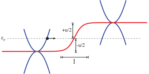
Figure 2: Low-energy band structure of a single valley on either side of the potential step. The Fermi energy is the same on both sides, causing an electron from the left side to tunnel through the barrier from the conductance band to the valence band on the right side.

Using the nearest-neighbour tight-binding approximation in the Slonczewski-Weiss-McClure parameterisation [16], one can write the Hamiltonian at a K point (for basis $(\phi_{A},\phi_{B2},\phi_{A2},\phi_{B})$) as

$${\cal H}_{\mathrm{4x4}}=\begin{pmatrix}-\xi\frac{\Delta}{2}\sigma_{z}+\hat{u}&\xi v\bm{\sigma}\cdot\bm{p}\\ \xi v\bm{\sigma}\cdot\bm{p}&\xi\frac{\Delta}{2}\sigma_{z}+\gamma_{1}\sigma_{x}+\hat{u}\end{pmatrix},$$ (1)

where $\bm{\sigma}=(\sigma_{x},\sigma_{y})$, $\bm{p}=(p_{x},p_{y})$ and $\xi$ is the Dirac point index ($\xi=+1$ for the valley around the $\mathrm{K}$ point, $-1$ for the valley around the $\mathrm{K^{\prime}}$ point, and throughout this paper we set $\hbar=1$). $v=\frac{\sqrt{3}}{2}a\gamma_{0}/\hbar$ and $\sigma_{i}$ are the Pauli spin matrices. Furthermore, $\Delta=\varepsilon_{2}-\varepsilon_{1}$ is the difference between the on-site energies in the two layers, $\varepsilon_{2}=\frac{1}{2}\Delta$, $\varepsilon_{1}=-\frac{1}{2}\Delta$, which produces a gap in the energy spectrum [17]. A potential term $\hat{u}=\mathbb{I}u$ is added along the diagonal to represent the electrostatic potential (we neglect inter-valley scattering between $\mathrm{K}$ and $\mathrm{K^{\prime}}$; $\mathbb{I}$ is the unit matrix). We assume that the interlayer coupling $\gamma_{1}$ is large compared to other energies in the system (which is reasonable for the low-energy regime near the Dirac points). Given that $\varepsilon\ll\gamma_{1}$ (where $\varepsilon$ is the energy of charge carriers), and with $\varepsilon=p^{2}/2m$, where $m=\gamma_{1}/2v^{2}$, we see that $(pv/\gamma_{1})^{2}\ll 1$. From this justification, we drop terms beyond quadratic in momentum in the following calculations. We assume a non-adiabatic system, with

$$a\ll l_{\perp}\ll(l,\lambda_{F}),$$ (2)

where $a$ is the lattice constant, $l$ the width of the step (see Fig. 2), $l_{\perp}=v/\gamma_{1}$, and $\lambda_{F}$ is the Fermi wavelength.

We use a Schrieffer-Wolff transformation [18] to map Eq. (1) in a 4D Hilbert space into a 2D subspace, creating an effective Hamiltonian. If we let ${\cal H}_{\mathrm{4x4}}={\cal H}^{0}+\delta{\cal H}$, with

$${\cal H}^{0}=\begin{pmatrix}H_{11}&0\\ 0&H_{22}\end{pmatrix},\qquad\delta{\cal H}=\begin{pmatrix}0&H_{12}\\ H_{21}&0\end{pmatrix},$$ (3)

we can then write the associated Green’s function as ${\cal G}_{\mathrm{4x4}}=(\varepsilon-{\cal H}_{\mathrm{4x4}})^{-1}=(\varepsilon-{\cal H}^{0}-\delta{\cal H})^{-1}$ and expand:

$${\cal G}_{\mathrm{4x4}} = (\varepsilon-{\cal H}^{0})^{-1}+(\varepsilon-{\cal H}^{0})^{-1}\delta{\cal H}(\varepsilon-{\cal H}^{0})^{-1}+$$ (4)

$$(\varepsilon-{\cal H}^{0})^{-1}\delta{\cal H}(\varepsilon-{\cal H}^{0})^{-1}\delta{\cal H}(\varepsilon-{\cal H}^{0})^{-1}+\cdots.$$

Given the basis that ${\cal H}_{\mathrm{4x4}}$ is constructed in, and that the low-energy quasiparticle transport is directly from atom A to B2 in the bilayer unit cell [1] (see Fig. 1), we wish to map ${\cal H}_{\mathrm{4x4}}$ onto the $H_{11}$ block matrix, using a Schrieffer-Wolff transformation. This has the effect of only keeping terms with an even number of $\delta{\cal H}$ components. The end result is that $G_{11}^{-1}=\varepsilon-H_{11}-H_{12}(\varepsilon-H_{22})^{-1}H_{21}$.

During this projection, the orthonormality of the wavevectors has to be preserved. To do this, we notice that $G_{11}^{-1}$ is an inverse Green’s function of the form

$$G_{11}^{-1} = \varepsilon-H_{11}+\Omega+\varepsilon\beta,$$

$$\beta = \frac{1}{\gamma_{1}^{2}}H_{12}H_{21},$$

$$\Omega = \frac{\xi\frac{\Delta}{2}}{\gamma_{1}^{2}}H_{12}\sigma_{z}H_{21}-\frac{1}{\gamma_{1}^{2}}H_{12}\hat{u}H_{21}$$ (5)

$$+\frac{1}{\gamma_{1}}H_{12}\sigma_{x}H_{21}.$$

We write an effective Schrödinger equation as $\varepsilon(1+\beta)|\psi\rangle=(H_{11}-\Omega)|\psi\rangle$. We wish to enforce $\langle\psi|1+\beta|\psi\rangle=|\psi|^{2}$ and $\langle\varphi|\psi\rangle=0$. Writing the wavefunction in terms of a new wavefunction $|\tilde{\psi}\rangle$, $|\psi\rangle=(1+\beta)^{-1/2}|\tilde{\psi}\rangle$. Inserting this result back into the effective Schrödinger equation gives us $H_{\mathrm{eff}}=(1+\beta)^{-1/2}(H_{11}-\Omega)(1+\beta)^{-1/2}$, which after Taylor expanding around $\beta$ up to ${\cal O}(\beta^{2})$ produces

$$H_{\mathrm{eff}}=H_{11}-\Omega-\left\{(H_{11}-\Omega),\frac{1}{2\gamma_{1}^{2}}H_{12}H_{21}\right\},$$ (6)

where the curly braces denote the anticommutator. The effective Hamiltonian can thus be calculated as

$$H_{\mathrm{eff}}= - \frac{1}{2m}\left[\sigma_{x}\left(-k_{y}^{2}-\partial_{x}^{2}\right)+2\mathrm{i}\sigma_{y}k_{y}\partial_{x}\right]$$ (7)

$$+ \xi\frac{\Delta v^{2}}{\gamma_{1}^{2}}|\bm{p}|^{2}\sigma_{z}-\xi\frac{\Delta}{2}\sigma_{z}+\hat{u}$$

$$+ \frac{v^{2}}{2\gamma_{1}^{2}}\left[(\bm{\nabla}^{2}u)+2\bm{\sigma}(\bm{\nabla}u\times\bm{p})\right]$$

$$+ \frac{v^{2}\xi}{4\gamma_{1}^{2}}\big{[}2\mathbb{I}(\bm{\nabla}\Delta)\times\bm{p}$$

$$-\sigma_{z}\left\{4\left((\bm{\nabla}\Delta)\cdot\bm{\nabla}+\Delta\bm{\nabla}^{2}\right)+(\bm{\nabla}^{2}\Delta)\right\}\big{]}.$$

The first two lines form the Hamiltonian found in Ref. [1] (neglecting trigonal warping). The additional correctional terms arise from the spatial dependence of $u$ and $\Delta$. Their derivation and the following analysis represent the subject and result of this paper.

The effective Hamiltonian in Eq. (7) can be simplified when $\lambda_{F}\gg l$. Terms with $|\bm{p}|^{2}\sim k_{F}^{2}$ can be dropped, given the length scales in this regime and the de Broglie relation. Now we wish to compare terms containing the potential $u$ and gap $\Delta$. To do this, we follow a simplified scheme to that defined in Ref. [17], modelling the bilayer on a substrate as a parallel plate capacitor.

Each layer of graphene has surface area $A$, and we take the dielectric constants of the material between the back gate and layer 1, and the bilayer, to be unity. Layer 1 has charge $Q=-n_{1}eA$, while layer 2 has charge $Q^{\prime}=-n_{2}eA$, where $n_{1}$ ($n_{2}$) is the density on layer 1 (2) (and $n=n_{1}+n_{2}$). The back gate and layer 1 are separated by a distance $L_{b}$, while the two layers are separated by a distance $c_{0}$. Applying a Gaussian surface around layer 1, the magnitude of the electric field is $E=Q/\varepsilon_{0}A$, where $\varepsilon_{0}$ is the permittivity of free space. The voltage due to this electric field is thus $QL_{b}/\varepsilon_{0}A$. The electric potential energy due to the back gate (thus, the potential $u$) is $u=eQL_{b}/\varepsilon_{0}A=n_{1}e^{2}L_{b}/\varepsilon_{0}$. We assume that the electric field from the back gate is screened poorly by layer 1, so applying the same analysis to layer 2, we find that the magnitude of the electric field is $E^{\prime}=Q^{\prime}/\varepsilon_{0}A$. The voltage produced by that electric field is $V^{\prime}=E^{\prime}c_{0}$, so the electric potential energy between the graphene layers (i.e., the gap) is $\Delta=n_{2}e^{2}c_{0}/\varepsilon_{0}$. If we assume that the charge density is evenly distributed between the layers, $n_{1}=n_{2}=n/2$, then $u/\Delta=L_{b}/c_{0}$. With $c_{0}\sim 0.3\mathrm{nm}$ and $L_{b}\sim 300\mathrm{nm}$, we find that $u\gg\Delta$. By writing $H_{\mathrm{eff}}$ in the form $H_{\mathrm{eff}}=\mathbb{I}A+\sigma_{x}B+\sigma_{y}C+\sigma_{z}D$, we compare each term and keep only the largest one in each group $A,B,C,D$. This produces an approximate Hamiltonian,

$$H_{\mathrm{app}}= - \frac{1}{2m}\left[\sigma_{x}\left(-k_{y}^{2}-\partial_{x}^{2}\right)+2\mathrm{i}\sigma_{y}k_{y}\partial_{x}\right]$$ (8)

$$+ \mathbb{I}\frac{k_{F}^{2}}{2m}\left[u+\frac{v^{2}}{2\gamma_{1}^{2}}\eta\left(\partial_{x}^{2}u\right)\right]$$

$$+ \sigma_{z}\left[-\xi\frac{\Delta}{2}+\eta\frac{v^{2}k_{F}^{2}}{2m\gamma_{1}^{2}}\left(\partial_{x}u\right)k_{y}\right],$$

where $\eta\in\{0,1\}$ and highlights the correctional terms.

An n-p junction can be formed with two back gates, schematically shown in Fig. 3. Each gate can independently create an electrostatic potential over that region of bilayer graphene. Given our chosen length scales in Eq. (2), we model the n-p junction as a Heaviside step function $\Theta(x)-(1/2)$, with its derivative the Dirac delta function. Thus, $u\approx(k_{F}^{2}/2m)[\Theta(x)-(1/2)]$, which also determines all additional terms in Eq. (7).

We define the problem in terms of plane waves on the left-hand and right-hand sides of the junction, $\psi_{1}$ and $\psi_{2}$ respectively:

$$\psi_{1} = \begin{pmatrix}1\\ a_{2}\end{pmatrix}\mathrm{e}^{\mathrm{i}k_{x}x}+b\begin{pmatrix}1\\ b_{2}\end{pmatrix}\mathrm{e}^{-\mathrm{i}k_{x}x}+c\begin{pmatrix}1\\ c_{2}\end{pmatrix}\mathrm{e}^{-\kappa x},$$

$$\psi_{2} = d\begin{pmatrix}1\\ d_{2}\end{pmatrix}\mathrm{e}^{-\mathrm{i}k_{x}^{\prime}x}+f\begin{pmatrix}1\\ f_{2}\end{pmatrix}\mathrm{e}^{\kappa^{\prime}x}.$$ (9)

The Hamiltonian in Eq. (7) has plane and evanescent wave solutions, and the quasiparticles are chiral, such that when they pass from the conductance band at the left of the interface to the valence band at the right, $k_{x}$ changes sign [3] (see Fig. 2).

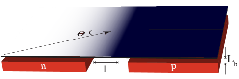
Figure 3: Angular dependence of quasiparticle transmission through an n-p junction.

With the step defined to be at $x=0$, we integrate Eq. (8) across it, $\int^{0+\delta}_{0-\delta}(\varepsilon-H_{\mathrm{app}})\mathrm{\,d}x$ and take the limit $\delta\rightarrow 0$. Matching the wavefunctions at either side of the junction ($\psi_{1}(0)=\psi_{2}(0)$), we obtain the boundary condition

$$0 = -\left.\frac{\sigma_{x}}{2m}\left(\partial_{x}\psi\right)\right|^{\psi_{2}(0)}_{\psi_{1}(0)}+\mathbb{I}\,\eta\frac{k_{F}^{2}v^{2}}{4m\gamma_{1}^{2}}\left(\frac{\psi_{1}^{\prime}(0)+\psi_{2}^{\prime}(0)}{2}\right)$$ (10)

$$-\sigma_{z}\eta\frac{v^{2}k_{F}^{2}k_{y}}{2m\gamma_{1}^{2}}\psi(0),$$

where the Fermi momentum $k_{F}=\sqrt{k_{x}^{2}+k_{y}^{2}}$ and

$$a_{2} = \frac{1}{\varepsilon-(u/2)}\left(\frac{k_{y}^{2}}{2m}-\frac{k_{x}^{2}}{2m}+\frac{\mathrm{i}k_{x}k_{y}}{m}\right),$$

$$b_{2} = a_{2}^{*},$$

$$c_{2} = \frac{1}{\varepsilon-(u/2)}\left(\frac{k_{y}^{2}}{2m}+\frac{\kappa^{2}}{2m}-\frac{\kappa k_{y}}{m}\right),$$

$$d_{2} = \frac{1}{\varepsilon+(u/2)}\left(\frac{k_{y}^{2}}{2m}-\frac{k_{x}^{\prime 2}}{2m}-\frac{\mathrm{i}k_{x}^{\prime}k_{y}}{m}\right),$$

$$f_{2} = \frac{1}{\varepsilon+(u/2)}\left(\frac{k_{y}^{2}}{2m}+\frac{\kappa^{\prime 2}}{2m}+\frac{\kappa^{\prime}k_{y}}{m}\right).$$ (11)

Using these equations, where $k_{x}=\sqrt{-k_{y}^{2}+2m[(u/2)-\varepsilon]}$, $k_{x}^{\prime}=\sqrt{-k_{y}^{2}+2m[(u/2)+\varepsilon]}$, $\kappa=\sqrt{k_{y}^{2}+2m[(u/2)-\varepsilon]}$, and $\kappa^{\prime}=-\sqrt{k_{y}^{2}+2m[(u/2)+\varepsilon]}$, we calculate the transmission probability for a symmetric junction $T(k_{y})=|d|^{2}$. We assume a wide strip, such that $k_{y}$ is invariant. We also set $\varepsilon=0$ in the middle of the barrier for simplicity. Using $k_{y}=k_{F}\sin(\theta)$ (see Fig. 3) we first calculate the transmission with only the leading-order terms in Eq. (10) (by setting $\eta=0$), finding agreement with Ref. [3] in that $T(\theta)=\sin^{2}(2\theta)$. Including the correctional terms from Eq. (10) by setting $\eta=1$, we obtain a correction to the incident angle at which perfect transmission is seen (see Fig. 4).

Taylor expanding the full analytical result for $T(\theta)$ around $\eta$, we find that only the first-order term is important and obtain a potential-dependent result (providing a good fit up to $u\approx 50\mathrm{meV}$):

$$T(\theta)\cong\sin^{2}(2\theta)-\frac{2u}{3\gamma_{1}}\sin(4\theta)\sin(\theta).$$ (12)

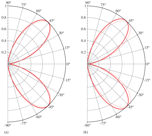
Figure 4: The dashed line shows the transmission probability without correctional terms applied. The solid line includes correctional terms. The dashed line shows perfect transmission at an angle of $45^{\circ}$ to the interface. (a) Transmission at $u=40\mathrm{meV}$. (b) Transmission at $u=80\mathrm{meV}$. Plotted with $\varepsilon=0$, $v\approx c/300$, $\gamma_{1}=0.4\mathrm{eV}$, $m=0.035\mathrm{m_{e}}$, $\Delta=0$.

Assuming a wide graphene sheet (that is, a width $w$ much greater than the length) and coherent quasiparticles, one can calculate the conductance from the transmission probability using the Landauer-Büttiker approach [19] (taking into account two valleys and two spins),

$$G=\frac{4e^{2}}{h}\sum_{n}|t_{n}|^{2}.$$ (13)

With $k_{y}=2\pi n/w$ (where $n$ is an integer), we can write this as an integral and calculate it using the full numerical transmission probability,

$$G=\frac{4e^{2}wk_{F}}{2\pi h}\int^{\pi/2}_{-\pi/2}\mathrm{\,d}\theta\cos(\theta)T(\theta)\cong 2.1\frac{e^{2}wk_{F}}{\pi h}$$ (14)

for $u=40\mathrm{meV}$. This is a slight reduction from $2.12e^{2}wk_{F}/\pi h$ for the case $\eta=0$. One can also calculate the Fano factor [20, 21] (the ratio of shot noise to Poisson noise; for a review see Ref. [22]) numerically:

$$F=\frac{\int_{-\pi/2}^{\pi/2}\mathrm{\,d}\theta\cos(\theta)T(\theta)(1-T(\theta))}{\int_{-\pi/2}^{\pi/2}\mathrm{\,d}\theta\cos(\theta)T(\theta)}\cong 0.241$$ (15)

for $u=40\mathrm{meV}$, showing a small increase compared to $F\cong 0.238$ when $\eta=0$ (see Fig. 5).

Figure 5: The Fano factor as a function of $u$, from a numerical calculation of the transmission probability for the same parameters as given in Fig. 4.

In conclusion, we have extended the earlier derived low-energy effective Hamiltonian for bilayer graphene to incorporate a spatially dependent electrostatic potential consistently. We calculate the angle-dependent transmission through an n-p junction and find $T(\theta)\cong\sin^{2}(2\theta)-(2u/3\gamma_{1})\sin(4\theta)\sin(\theta)$. Perfect transmission is still seen, but at a slightly increased angle. The conductance is slightly reduced to $G\cong 2.1e^{2}wk_{F}/\pi h$, whereas the Fano factor is slightly increased to $F\cong 0.241$ (both for $u=40\mathrm{meV}$).

The author thanks V. I. Fal’ko and V. Cheianov for supervision during this project and H. Schomerus, E. McCann and J. Cserti for useful discussions. The author thanks Lancaster University for financial support.

References

[1]
E. McCann, V. I. Fal’ko, Phys. Rev. Lett. 96 (2006) 86805.
[2]
A. Geim, K. S. Novoselov, Nat. Mater. 6 (2007) 183–191.
[3]
M. I. Katsnelson, K. S. Novoselov, A. Geim, Nat. Phys. 2 (2006) 620–625.
[4]
V. V. Cheianov, V. I. Fal’ko, Phys. Rev. B 74 (2006) 41403.
[5]
V. V. Cheianov, V. I. Fal’ko, B. L. Altshuler, Science 315 (2007) 1252.
[6]
J. Cayssol, B. Huard, D. Goldhaber-Gordon, Phys. Rev. B 79 (2009) 075428.
[7]
N. Stander, B. Huard, D. Goldhaber-Gordon, Phys. Rev. Lett. 102 (2009) 026807.
[8]
B. Huard, J. A. Sulpizio, N. Stander, K. Todd, B. Yang, D. Goldhaber-Gordon,
Phys. Rev. Lett. 98 (2007) 236803.
[9]
J. R. Williams, L. DiCarlo, C. M. Marcus, Science 317 (2007) 638–641.
[10]
J. Cserti, A. Palyi, C. Peterfalvi, Phys. Rev. Lett. 99 (2007) 246801.
[11]
C. Peterfalvi, A. Palyi, J. Cserti, Phys. Rev. B 80 (2009) 075416.
[12]
M. M. Fogler, D. S. Novikov, L. I. Glazman, B. I. Shklovskii, Phys. Rev. B 77
(2008) 075420.
[13]
L. M. Zhang, M. M. Fogler, Phys. Rev. Lett. 100 (2008) 116804.
[14]
R. V. Gorbachev, A. S. Mayorov, A. K. Savchenko, D. W. Horsell, F. Guinea, Nano
Lett. 8 (2008) 1995–1999.
[15]
I. Snyman, C. W. J. Beenakker, Phys. Rev. B 75 (2007) 045322.
[16]
J. Slonczewski, P. Weiss, Phys. Rev. 109 (1958) 272–279.
[17]
E. McCann, Phys. Rev. B 74 (2006) 161403.
[18]
J. R. Schrieffer, P. A. Wolff, Phys. Rev. 149 (1966) 491–492.
[19]
M. Büttiker, Phys. Rev. Lett. 57 (1986) 1761–1764.
[20]
U. Fano, Phys. Rev. 72 (1947) 26–29.
[21]
J. Tworzydlo, B. Trauzettel, M. Titov, A. Rycerz, C. W. J. Beenakker, Phys.
Rev. Lett. 96 (2006) 246802.
[22]
Y. M. Blanter, M. Büttiker, Phys. Rep. 336 (2000) 1–166.