Variable stars, distance scale, globular clusters

Abstract

In these concluding remarks we concentrate on the current state of variable star studies including halo and globular-cluster variables, touch on some problems of the distance scale, and propose a new improvement to the well-known Baade-Wesselink method of determining the radii of variable stars.

autadxandAuthor Index

¹Moscow State University, Faculty of Physics, Moscow, Russia
²Sternberg Astronomical Institute, Moscow, Russia

1. Introduction

B.V.Kukarkin’s scientific interests concentrated mainly around variable stars, globular star clusters, and stellar populations. His first experience in variable star study as an amateur astronomer grew with time into a serious engagement into one of the most impressive Russian and Soviet astronomical projects - the General catalog of variable stars (GCVS). Kukarkin, together with his colleague and friend Pavel Parenago, were the initiators of this long-term and tedious work of great importance. Nowadays GCVS remains a very popular and valuable knowledge source on different types of variable stars and accumulates observational data that may serve as a potential source of insight into some special evolutionary stages of stars and physical processes involved.

In recent years, variable stars have been outlining the frontiers of modern astrophysics as ”beacons” of stellar evolution. For example, astro-seismological data are used to test the theories of stellar structure and evolution; different types of variable stars serve as indicators of advanced evolutionary stages on the CMD, and observations of evolutionary period changes in classical Cepheids and secular variability of post-AGB stars — predecessors of planetary nebulae — provide unique information on stellar evolution. All fields of modern astrophysics demonstrate the need for variable-star databases.

Serious problems that the authors of the GCVS had to address and that were associated with the classification of variable stars, gathering the data and updating the database, and with catalog’s compilation have already been discussed in this meeting by N.N.Samus. The GCVS now includes more than 60000 entries. Future difficulties are expected to be more serious than those of the past. For example, the ASAS-3 project has produced more than 30000 new suspected variables; and GAIA mission will result in approximately $10^{8}$ new variables in total – maybe, it will detect $\sim~{}10^{4}-10^{5}$ new variables every day. Russian space mission LYRA and many other international all-sky space and ground-based dedicated deep-sky surveys raise a lot of new large-scale problems that the GCVS team had not to face until now. Huge data sets, the ever increasing photometric accuracy accompanied by the sharp increase in the number of variability phenomena discovered require fundamentally new solutions, which must involve close international collaboration. The main features of the virtual observatory approach (unification of query and output formats) and the development of new automatic classification schemes based on self-learning algorithms and neural networks may prove to be of great importance for solving future problems.

2. Halo variable stars

RR Lyrae pulsating variables represent the old stellar population in galactic halos, thick disks and globular clusters. These stars populate a narrow region in the CMD - the intersection of cluster horizontal branch (HB) with the instability strip, and their energy sources are helium core and hydrogen shell burning. This stage lasts approximately 100 Myr and can be considered as some kind of the ”second main sequence”, by the contrast with the other, relatively short-lived advanced stages. The luminosities of RR Lyrae in an individual cluster differ only slightly, with a characteristic scatter in absolute magnitudes amounting to $\pm 0.15^{m}$. As was first suggested by Christy (1966) and confirmed by more recent theoretical track calculations (Vandenbergh et al. 2000), the optical luminosity of HB stars strongly depends on their chemical abundance, and hence the metallicity $[Fe/H]$ and $[\alpha/Fe]$ ratio are key parameters. The slope of the $M-[Fe/H]$ relation was estimated using different methods including the Baade-Wesselink technique and direct HIPPARCOS and HST FGS3 parallax measurements. Observations appear to support theoretical predictions and suggest a nearly universal slope for the $M-[Fe/H]$ relation from optics to NIR (Cacciari and Clementini 2003; Catelan et al. 2004), with $dM/d[Fe/H]\approx(+0.20\pm 0.04)^{m}/dex$. In the NIR RR Lyrae, like classical and Type II Cepheids, show a period luminosity ($M-logP$) relation best revealed by observations of RR Lyraes in globular clusters (Frolov and Samus 1998) with a slope of $dM_{K}/dlogP\approx(-2.34\pm 0.07)^{m}$.

The statistical-parallax technique offers new opportunities for the refinement of the luminosities of RR Lyrae variables (see a comprehensive review by Gould and Popovski 1998). The above authors analyzed the eventual biases of this method due to the kinematical inhomogeneity of the original sample and other factors. Cacciari and Clementini (2003) noted poor discrimination of halo and thick disk variables, and a large fraction of ”accretion” population among observed halo stars. Two halo subsystems would have different dynamical characteristics and origins: the fast rotating subsystem associated with the Galactic thick disk, and the slowly (possibly retrograde) rotating subsystem belonging to the accreted outer halo (Bell et al. 2008). Any kinematical inhomogeneity in the sample used may introduce unpredictable systematical errors into the derived distance scale. The statistical parallax technique, very powerful and robust in itself, needs more adequate kinematical models for halo populations and more extensive RR Lyrae samples with good radial velocities and proper motions, and seems to be a very important task for future investigations. The kinematics the of local RR Lyrae population and the associated distance scale was analyzed in details by Dambis and Rastorguev (2001) and Dambis (2009). Apparently, the best way to account for the biases of the statistical parallax technique consists in applying it to simulated inhomogeneous data sets and estimating the systematical errors.

Kukarkin used the distances of the globular clusters calculated from the original Christy’s (1966) idea that the luminosity of stars at the HB stage strongly depends on metallicity (with the overestimated slope of $dMV/d[Fe/H]=0.38^{m}$), to calibrate the luminosities of the Cepheids in globular clusters (Kukarkin and Rastorguev 1972, 1973). This relatively poor sample is now considered to be a mixture of stars of different nature: low-mass stars evolving from the HB and entering the instability strip (above horizontal branch variables, AHB), and low-mass stars on the asymptotic giant branch stage (AGB) looping inside the IS during the thermal instability phase (true Type II Cepheids). The above authors noted that the $M_{V}$ - log P relation has a break near the 7-8 day period. This is quite similar to what we see in the case of classical Milky Way and LMC Cepheids, which show a pronounced slope break near the 10-day period (Sandage et al. 2004). The slope difference may complicate the use of Cepheids as standard candles. Nonlinear calculations of Cepheid models also seem to support the idea of two Cepheid families. Unfortunately, in the last three decades the progress in the detailed studies of Type II Cepheids and Cepheids in globular clusters was by far not as impressive as with type-I Cepheids. For example, there is even a certain confusion regarding the very name of the class of type II Cepheid variables: some investigators prefer to use the term short-period Cepheids for BL Her type stars rather than for AHB Cepheids. We should mention valuable data on Type II Cepheids in the galactic field, in globular clusters and in nearby galaxies derived from recent NIR observations (Matsunaga et al. 2006, 2009). These data have substantially expanded the sample Type II cepheids; the results seem not to confirm early suggestion of the existence of any PL breaks and demonstrate small scatter of $JHK_{S}$ PL relations. The metallicity effect in the luminosities of Type II Cepheids is now discussed. We expect Type II Cepheids to be potentially good ”standard candle” candidates and useful tools for estimating distances to halo populations of external galaxies.

3. Variable stars as evolution probes

In many cases stellar variability is a ”lighthouse” of stellar evolution. The instability strip that crossing the entire CMD is the best argument. Classical Cepheids and other pulsating variables with relatively stable cycles (RR Lyrae, W Vir, etc.) seem to be good probes of stellar evolution which is accompanied by the rearrangement of stellar interiors. It is well known that the lines of constant periods are not parallel to the evolution tracks, and hence the star MUST change its pulsation period. The search for secular period changes was among the first B.V. Kukarkin’s scientific activities of the 1930th. Nowadays, Leonid Berdnikov and David Turner made a decisive contribution to this field (Turner and Berdnikov 2004; Turner et al. 2006). The new data obtained as a result of their multicolor photometric monitoring of classical Cepheids supplemented them by ”historical” data ”recorded” in old photographic plates allowed them in many cases to study period changes over 150-years long time intervals. The above authors reveal secular period changes in many classical Cepheids, often masked by spurious period variations. The sign and magnitude of period change rate are unique indicators of the evolution stage – the number of the crossing of the instability strip and the speed of evolution along the track.

Careful inspection of CMD tracks for massive stars shows a number of successive loops crossing the instability strip with large differences in Cepheid’s luminosity ($\sim 1^{m}$). It is now widely recognized that the identification of the crossing number can reduce appreciably the scatter of the PL relation. The study of period changes for different types of pulsating variables can be viewed as a promising way to improve the period-luminosity relation of Cepheids as the best ”standard candles”, and universal distance scale in general. Cepheids and other types of pulsating variables are not the only objects to exhibit evolutionary effects; Arkhipova et al. (2007) have recently pointed out that some supergiants with infrared excess also show very fast evolution from the AGB to Planetary Nebulae on the CMD, which is accompanied by photometric and spectroscopic trends over a short time interval (dozen of years).

Great importance of stellar evolution and distance scale studies makes the scanning and digitizing of historical astro-plates one of the foremost observational tasks.

4. Globular clusters and galactic halo populations

Globular star clusters have always been considered natural laboratories of stellar evolution and stellar dynamics. The old idea of globular star clusters as typical examples of simple stellar population (SSP) has greatly changed in the past years. In the 1960ies, there was no direct observational evidence for the presence of binary stars among cluster members. Only after 1975, when X-ray emission was detected from the central parts of densest globular clusters, it occurred that the explanation may involve binary systems with compact objects. Now binary population seems to be typical for globular clusters. Binarity explains the phenomenon of ”blue straggler” stars (BSS). More than 3000 BSS were have been detected in  60 thoroughly studied clusters (Piotto et al. 2004). Peculiarities of the radial distribution of BSS relative to red-giant stars and the relation between BSS populations and some of the cluster properties imply two scenarios of their production: mass exchange in collisional and primordial binaries (Davies et al. 2004). Large relative frequency of BSS in the halo field as compared to cluster population is also a very interesting result. Close binaries seem to be a typical population among blue horizontal branch (BHB) and extended horizontal branch (EHB) stars (Ferraro et al. 2001). Note also that the fraction of binaries in old open clusters is higher than in globular clusters: according modern data, the binary fraction in old open cluster cores is estimates at $>11\%$, whereas the overall fraction ranges from $35\%$ to $70\%$ (Sollima et al. 2009).

Recent photometric and spectroscopic observations with HST and VLTs revealed multiple main sequences and turnoff-points in some globular clusters including $\omega Cen,NGC2808$ etc. (Bedin et al. 2004, Piotto et al. 2005, Villanova et al. 2007, Piotto et al. 2007). Even more exciting was the detection of two populations with different $[Ca/Fe]$ among red giant stars in the nearest ”normal” globular cluster $NGC6121=M4$ (Marino et al. 2008). These observations are indicative of complex star formation processes in globular clusters, maybe of multiple populations, which can be closely related to the cluster dynamical history and some special properties, such as escape velocity.

The old view of globular clusters as a very homogeneous populations in the Milky Way and external galaxies has been drastically changed by recent studies of galaxy-formation processes, beginning from very high redshifts. Theoretical simulations of galaxy formation in the $\Lambda CDM$ scenario (early clustering of dark matter, accretion of ordinary matter to DM clumps) have shown that at early epochs multiple mergers – major and minor – took place and eventually shaped the recent ”faces” of spiral and elliptical galaxies. These calculations also show the formation of cluster-like clumps (Kravtsov and Gnedin 2005). Recent SDSS data have clearly shown that minor merger events occur just now, and stellar traces of the disruption of dwarf galaxies and globular clusters in the Milky-Way tidal field can be identified among the thick disk and halo populations (Bell et al. 2008, Koposov and Belokurov 2008, Smith at al. 2009). The study of peculiarities in the kinematics and chemical abundances made it possible to identify ”accretion” populations among galactic globular clusters, thick-disk stars and even among the nearest stars (Marsakov and Borkova 2005ab, Marsakov and Borkova 2006). Dr. Clementini (see paper in this book) demonstrated how the populations of RR Lyrae of OoI/OoII types helps to establish the merger history and understand the Milky-Way formation via mergers of faint dwarf spheroidal galaxies. The age and abundance differences between ”accreting” clusters originated in dwarf satellites and ”normal” galactic globular clusters could provide an insight into the so called problem of the ”second parameter”, which is responsible for the HB morphology.

The kinematics of distant halo objects – dwarf Milky-Way satellites, globular clusters, RR Lyrae variables, constant BHB stars – which are easily identifiable among field stars, serve as a tool to set additional constraints onto the gravitational potential of the Milky Way and the contribution of dark matter. An important work was done by Battaglia et al. (2005) who used Jeans equations and radial velocities of about 250 distant objects to find the best fit for the dependence of velocity dispersions on Galactocentric radius. They found the velocity distribution to be dominated by transverse motions at large distances and estimated the total Milky-Way mass at $\sim 10^{12}M_{sun}$. Recently Dambis (see paper in this book) used radial-velocity and proper-motion data (adopted from the last SDSS data release) for a large sample of halo objects (including BHB stars) to estimate the local Milky Way rotation velocity and the shape of the velocity ellipsoid out to a Galactocentric distance of $\sim 40\;kpc$. He demonstrated that 3D-velocities are good enough to constrain flat rotation curve with $V_{rot}\approx 195\pm 10\;km/s$ and confirm large Milky Way mass dominated by DM on large distances.

5. Distance scale

The reliability of the universal distance scale is of exclusive value to all astrophysics, stellar astronomy and cosmology. It is well known that Cepheids are objects of exceptional importance because their PL relation makes them good ”standard candles” in distant galaxies. There are a number of ways to determine the period-luminosity (PL) and period-luminosity-color (PLC) relations from observational data (see the review of Sandage and Tammann, 2006). It is common practice to scale all distance scales of different ”candles” to the LMC distance. One of the HST key projects was devoted to precise LMC distance and Hubble constant measurements (Freedman et al. 2001). As a result, it emerged with ”mean” LMC distance modulus $(m-M)_{0}=18.5\pm 0.10^{m}$. Schaefer (2008) analyzed all LMC distance estimates and concluded that after 2001 this average value has been generally accepted, and all reported LMC distance estimates clustered more tightly around the ”mean” value, actually too tightly with an appreciable excess of too precise measurements. Schaefer used Kolmogorov-Smirnov (K-S) test to demonstrate that this clustering may be the symptom of a worrisome problem, which is well known as the ”band-wagon” effect or the correlation between papers resulting from underestimated systematic errors. Schaefer mentioned that adequate treating of the systematic uncertainties is one of the serious problems that can greatly affect the estimates of the distances and other astrophysical parameters.

Given that the calculation of pulsation radii can improve the luminosity calibrations for Cepheids and RR Lyraes, I propose a new approximation for the projection factor (PF) used in all implementations of the W.Baade-W.Becker-A.Wesselink-L.Balona (BBWB) technique to calculate the radius difference from the radial-velocity curve. This technique can be used in the surface-brightness method (Baade 1931) and in the modeling of the light curve – and also in its maximum-likelihood implementation (Balona 1977).

The PF value calculated by integrating the flux across the stellar limb depends on limb darkening coefficient, $\epsilon$ (from $D(\varphi)=1-\epsilon+\epsilon\;cos\varphi,\;\varphi$ is the angle between line-of-sight direction and the normal vector to the surface element), and the velocity of the photosphere, $dr/dt$. The intrinsic line profile is broadened by any spectral instrument, and usually we approximate the profile by a Gaussian curve to measure the radial velocity as the coordinate of the maximum. This is the standard technique used by CORAVEL-type spectrographs (Tokovinin 1987). I used these elementary geometric considerations to show that the measured radial velocity should additionally depend on the instrument spectral line width, $S_{0}$, so PF value should be ”adjusted” to the spectrograph used for radial-velocity measurements.

We calculated the PF values for $2.5<|dr/dt|<60\;km/s;\;0<\epsilon<1;\;4<S_{0}<8\;km/s$. We see from Fig. 1 that the maximum of normal approximation is shifted relative to the tip of the line profile. This shift depends on $dr/dt$ and $S_{0}$. Figure 2 shows that the calculated PF values differ considerably from the ”standard” and widely used value of $PF=1.31$. Variations of PF were reported earlier by Nordetto et al. (2004) and others. The PF variation with the period, mentioned earlier by some authors, possibly reflects PF variation as a function of the limb-darkening coefficient.

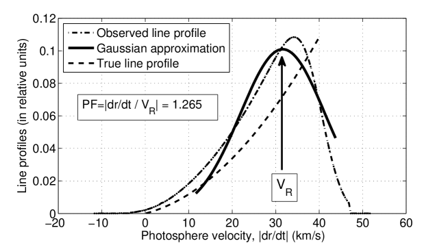
Figure 1.: An example: intrinsic line profile ($\epsilon=0.75,dr/dt=40\;km/s$), observed line profile and its Gaussian approximation (with the spectrograph instrumental line width $S_{0}=4\;km/s$). Measured $V_{R}$ value is indicated by the arrow; the PF value is shown.

The bottom panel in Fig. 2 shows the variation of the line width with the photosphere velocity, and this effect was observed during our measurements of the correlation profile of bright Cepheids with the ILS CORAVEL-type spectrometer constructed by Tokovinin (1987). The upper panel clearly shows large variation of PF values in the interval from $1.23$ to $1.43$, which does not confirm Groenewegen’s (2007) result that PF can be assumed to be constant, $PF=1.26\pm 0.05$.

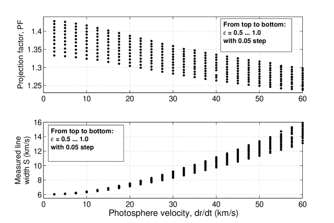
Figure 2.: Projection factor, PF, and measured line width, $S$, as a function of $dr/dt$ for instrumental width $S_{0}=6\;km/s$ and for different values of limb darkening coefficient $0.5<\epsilon<1$.

A useful analytic approximation for the projection factor seems to be of crucial importance for calculating the radii of Cepheids and RR Lyraes using the surface brightness technique and Balona’s (1977) maximum-likelihood method of light curve modeling. A careful inspection of PF as a function of $dr/dt$ leads us to a three-parameter exponential approximation. Modeling of the line profiles for many sets of input parameters (see above) allowed us to derive the following general formula:

$$PF\approx a_{1}\cdot exp(-(dr/dt)^{2}/(2\cdot a_{2}^{2}))+a_{3},$$

where $a_{1},a_{2},a_{3}$ are functions of $\epsilon,S_{0}$:

$a_{1}\approx-0.068\cdot\epsilon-0.0078\cdot S_{0}+0.217$

$a_{2}\approx+1.69\cdot\epsilon+2.477\cdot S_{0}+9.833$

$a_{3}\approx-0.121\cdot\epsilon+0.009\cdot S_{0}+1.297$

The overall RMS residual of the calculated PF value from this analytic expression is about $\pm 0.003$. In the same way, we derived the following approximation for $S$:

$$S\approx b_{1}\cdot(dr/dt)^{2}+b_{2}\cdot|dr/dt|+b_{3},$$

where

$b_{1}\approx-0.001\cdot\epsilon+0.00\cdot S_{0}+0.0027$

$b_{2}\approx-0.036\cdot\epsilon-0.011\cdot S_{0}+0.152$

$b_{3}\approx+0.215\cdot\epsilon+1.048\cdot S_{0}-0.743$

with the RMS of approximation equal to $\pm 0.12$. In practice, the PF for measured radial velocity should be determined by iterations for known $S_{0}$ value.

This work was partly supported by the RFBR grant 08-02-00738.

References

- Arkhipova et al. (2007) Arkhipova, V.P., Esipov, V.F., Ikonnikova, N.P. et al. 2007, AstL, 33,604
- Baade (1931) Baade, W. 1931, Mittel.Hamburg.Sternw., 6, 85
- Balona (1977) Balona, L. 1977, MNRAS, 178, 231
- Battaglia et al. (2005) Battaglia, G., Helmi, A., Morrison, H. et al 2005, MNRAS, 364, 433
- Bedin et al. (2004) Bedin, L.R., Piotto, G., Anderson, J et al. 2004, ApJ, 605, L125
- Bell et al. (2008) Bell, E.F, Zucker, D.B., Belokurov, V. et al. 2008, ApJ, 680, 295
- Cacciari & Clementini (2003) Cacciari, C., & Clementini, G. 2003, Stellar Candles for the Extragalactic Distance Scale (eds. D.Alloin and W.Gieren), Springer, Lecture Notes in Physics, 635, 105
- Catelan et al. (2004) Catelan, M., Pritzl, B.J., & Smith, H.A. 2004, ApJS, 154, 633
- Christy (1966) Christy, R.F. 1966, ApJ, 144, 108
- Dambis & Rastorguev (2001) Dambis, A.K., & Rastorguev A.S. 2001, AstL, 27,108
- Dambis (2009) Dambis, A.K. 2009, MNRAS, 396, 553
- Davies et al. (2004) Davies, M.B., Piotto, G., & de Angeli, F. 2004, MNRAS, 349, 129
- Ferraro et al. (2001) Ferraro, F.R., Diamico, N., & Possenti, A. 2001, ApJ, 561, 345
- Freedman et al. (2001) Freedman, V.L., Madore, B.F., Gibson, B.K. et al. 2001, ApJ, 553, 47
- Frolov & Samus (1998) Frolov, M.S., & Samus, N.N. 1998, AstL, 24, 174
- Gould & Popovski (1998) Gould, A., & Popovsky, P. 1998, ApJ, 508, 844
- Groenewegen (2007) Groenewegen, M.A.T. 2007, A&A, 474, 975
- Koposov & Belokurov (2008) Koposov, S., & Belokurov, V. 2008, Galaxies in the Local Volume (Astrophysics and Space Science Proceedings), Springer, 195
- Kravtsov & Gnedin (2005) Kravtsov, A.V., & Gnedin, O.Y. 2005, ApJ, 623, 650
- Kukarkin & Rastorguev (1972) Kukarkin, B.V., & Rastorguev, A.S. 1972, Perem. Zvezdy Byull., 18, 383
- Kukarkin & Rastorguev (1973) Kukarkin, B.V., & Rastorguev, A.S. 1973, Variable stars in globular clusters and in related systems, Proc. IAU Colloq No.21 (eds. J.D.Fernie), Toronto, 1972, 180
- Marino et al. (2008) Marino, A.F., Villanova, S., Piotto, G. et al. 2008, A&A, 490, 625
- Marsakov & Borkova (2005) Marsakov, V.A., & Borkova, T.V. 2005, From Lithium to Uranium: Elemental Tracers of Early Cosmic Evolution (IAU Symp. Proc., eds Hill, V.; Francois, P.; Primas, F.), 228, 543
- Marsakov & Borkova (2005) Marsakov, V.A., & Borkova, T.V. 2005, AstL, 31, 515
- Marsakov & Borkova (2006) Marsakov, V.A., & Borkova, T.V. 2006, Astron. Astropys. Trans., 25, 149
- Matsunaga et al. (2006) Matsunaga, N., Fukushi, S., Nakada, Y. et al. 2006, MNRAS, 370, 1979
- Matsunaga et al. (2009) Matsunaga, N., Feast, M.W., & Menzies, J.W. 2009, MNRAS, 397, 933
- Nardetto et al. (2007) Nardetto, N., Mourard, D., Mathias, P. et al. 2007, A&A, 471, 661
- Piotto et al. (2004) Piotto, G., De Angeli F., King, I.R. et al. 2004, ApJ, 604, L109
- Piotto et al. (2005) Piotto, G., Villanova, S., Bedin, L.R. et al. 2005, ApJ, 621, 777
- Piotto et al. (2007) Piotto, G., Bedin, L.R., Anderson, J. et al. 2007, ApJ, 661, L53
- Sandage et al. (2004) Sandage, A., Tammann, G.A., & Reindl, B. 2004, A&A, 424, 43
- Sandage & Tammann (2006) Sandage, A., & Tammann, G.A. 2006, ARA&A, 44, 93
- Schaefer (2008) Schaefer, B.E. 2008, AJ, 135, 112
- Sollima et al. (2009) Sollima, A., Carbalo-Bello, J.A., Beccari, F.R. et al. 2009, arXive:0909.1277v1
- Smith et al. (2009) Smith, M.C., Evans, N.W., Belokurov, V. et al. 2009, MNRAS, 399, 1233
- Tokovinin (1987) Tokovinin, A.A. 1987, SvA, 31, 98
- Turner & Berdnikov (2006) Turner, D.G., & Berdnikov, L.N. 2004, A&A, 423, 335
- Turner et al. (2006) Turner, D.G., Abdel-Sabour, A.-L., & Berdnikov, L.N. 2006, PASP, 118, 410
- Vandenberg et al. (2000) Vandenberg, D.A., Swenson, F.J., Rogers, F.J. et al. 2000, ApJ, 592, 430
- Villanova et al. (2007) Villanova, S., Piotto, G., King, I.R. et al. 2007, ApJ, 663, 296