Diagrammatic theory for Periodic Anderson Model.
Stationary property of the thermodynamic potential

Abstract

Diagrammatic theory for Periodic Anderson Model has been developed, supposing the Coulomb repulsion of $f-$ localized electrons as a main parameter of the theory. $f-$ electrons are strongly correlated and $c-$ conduction electrons are uncorrelated. Correlation function for $f-$ and mass operator for $c-$ electrons are determined. The Dyson equation for $c-$ and Dyson-type equation for $f-$ electrons are formulated for their propagators. The skeleton diagrams are defined for correlation function and thermodynamic functional. The stationary property of renormalized thermodynamic potential about the variation of the mass operator is established. The result is appropriate as for normal and as for superconducting state of the system.

I Introduction

The study of the systems with strongly correlated electrons has become in the last time one of the central problem of condensed matter physics. One of the most important models of strongly correlated electrons is periodic Anderson model (PAM)^[1]. This model is used to describe the physics of mixed valence systems, heavy fermion compounds, high-temperature superconductivity as well as other phenomena in which the strong Coulomb repulsion of the localized electrons is present. This model describes the intermetallic compounds which contain magnetic moments of rare earth or actinide ions included in the host metal. This ions have a partially filled $f-$ shell and can be considered as scattering centers for conduction electrons of the host metal. Because of the strong Coulomb repulsion of the electrons with opposite spins located at the same site of lattice the magnetic ion electrons are strongly correlated. There is also the hybridization of states between the uncorrelated conduction electrons and localized correlated ones when both of them are present on the same lattice site. Magnetic properties of the impurities ions affect in a different manner the properties of the host matrix and of the system as a whole. For different regime of physical parameters, determined by Coulomb local interaction, hybridization of the wave functions and exchange interaction, it is possible to obtain different classes of the system phases.

There are already an enormous number of approximate methods and approaches devoted to PAM, as perturbation expansions, static and dynamic mean field theories, variational and numerical approaches, large $N$ expansion , slave boson methods, non crossing approximations (NCA), Bogoliubov inequality method and others. Also some exact results are known, obtained in special with the Bethe ansatz, renormalization group methods and Bogoliubov inequality method. We will not enlarge upon the most essential stages in the development of this model because exists a number of consistent reviews ^[2-7] and books ^[8,9] on this field and we shall use the references to previous our papers.

II Model Hamiltonian

We consider the simplest form of PAM with a spin degeneration of the level of localized $f-$ electrons, a simple energy band of conducting $c-$ electrons, Coulomb one-site repulsion $U$ of correlated $f-$ electrons with opposite spins and one-site hybridization between both group of electrons of this system. The hamiltonian of the system reads:

$$H = H_{c}^{0}+H_{f}^{0}+H_{int},$$

$$H_{c}^{0} = \sum\limits_{\mathbf{k}\sigma}\epsilon(\mathbf{k})\ C_{\mathbf{k}\sigma}^{+}C_{\mathbf{k}\sigma},$$

$$H_{f}^{0} = \epsilon_{f}\sum\limits_{i\sigma}n_{i\sigma}+U\sum\limits_{i}n_{i\uparrow}n_{i\downarrow},$$ (1)

$$H_{int} = V\sum\limits_{i\sigma}\left(C_{i\sigma}^{+}f_{i\sigma}+f_{i\sigma}^{+}C_{i\sigma}\right),$$

where

$$\epsilon(\mathbf{k}) = \overline{\epsilon}(\mathbf{k})-\mu,\epsilon_{f}=\overline{\epsilon}_{f}-\mu,$$

$$n_{i\sigma} = f_{i\sigma}^{+}f_{i\sigma},$$ (2)

$$C_{i\sigma} = \frac{1}{\sqrt{N}}\sum\limits_{\mathbf{k}}\exp{(-i\mathbf{k}\mathbf{R_{i}})}C_{\mathbf{k}\sigma}.$$

Here $V$ is the hybridization amplitude assumed constant. We have indicated with $C_{i\sigma}^{+}(f_{i\sigma}^{+})$ the creation operator for an uncorrelated (correlated) electron with spin $\sigma$ and $i$ lattice site, $n_{i\sigma}$ is the number operator for $f-$ electrons, $\epsilon(\mathbf{k})$ is the band energy with momentum $\mathbf{k}$ of conductivity electrons spread on the entire width $W$ of the band. $\epsilon_{f}$ is the energy of localized electrons. Both these energies are evaluated with respect to the chemical potential $\mu$.

The approach proposed in this paper generalizes the diagrammatic theory of normal and superconducting phases of strongly correlated systems proposed in previous papers ^[10-19].

The strong on-site repulsion $U$ between $f-$ electrons of opposite spins is the main term in the Hamiltonian.

As the conduction electrons can belong not only to the $s-$ but also to the $d-$ atomic shell, their Coulomb repulsion can also be important. In this case the extended PAM must be used ^[20]. For simplicity the correlations of $c-$ electrons are not considered and one subsystem is of $c-$ uncorrelated and the second of $f-$ correlated electrons. Because of strong localization of the $f-$ electrons they cannot hope from one lattice site to another and their delocalization is due only to the hybridization of the $f-$ and $c-$ states with matrix element $V$. It is obvious that at $V\neq 0$ in the given model with two subsystems superconductivity arises simultaneously in both subsystems.

In the present paper we develop the thermodynamic perturbation theory for the system in the superconducting state with Hamiltonian (1) under the assumption that the term responsible for hybridization of $c-$ and $f-$ electrons is a perturbation.

The Hamiltonian $H_{c}^{0}$ of the uncorrelated $c-$ electrons is diagonal in band representation, where as the Hamiltonian $H_{f}^{0}$ is diagonalized by using Hubbard transfer operators ^[21]. Therefore in the zeroth-order of the perturbation theory the statistical operator of grand canonical ensemble of the system is factorized in the momentum representation for $c-$ and in local representation for $f-$ electrons:

$$\exp{[-\beta(H_{c}^{0}+H_{f}^{0})]} = \prod\limits_{\mathbf{k}\sigma}\exp{(-\beta H_{c\sigma}^{0}(\mathbf{k}))}\times$$

$$\times\prod\limits_{i}\exp{(-\beta H_{f}^{0}(i))},$$

$$H_{c\sigma}^{0}(\mathbf{k}) = \epsilon(\mathbf{k})\ C_{\mathbf{k}\sigma}^{+}C_{\mathbf{k}\sigma},$$ (3)

$$H_{f}^{0}(i) = \epsilon_{f}\sum\limits_{\sigma}n_{i\sigma}+Un_{i\uparrow}n_{i\downarrow},$$

We use the series expansion for evolution operator:

$$U(\beta) = T\exp(-\int\limits_{0}^{\beta}H_{int}(\tau)d\tau).$$ (4)

in the interaction representation for electron operators ($a=c,f$):

$$a(x)=e^{\tau H^{0}}a(\mathbf{x})e^{-\tau H^{0}},\overline{a}(x)=e^{\tau H^{0}}a^{+}(\mathbf{x})e^{-\tau H^{0}}.$$ (5)

Here by $x$ means ($\mathbf{x},\sigma,\tau$).

We shall denote by $\left\langle TAB...\right\rangle_{0}$ the thermodynamic average with zeroth-order statistical operator (3) of the chronological product of electron operators $(AB...)$. Such averages are calculated independently for $c-$ and $f-$ operators with using for $c-$ electrons the Wick Theorem of weak quantum field theory and by using for $f-$ electrons the Generalized Wick Theorem (GWT) proposed by us in papers ^[10-13] for strongly correlated electron systems.

In the superconducting state, unlike the normal one, nontrivial statistical averages of operator products with even total number but inequal number of creation and annihilation electron operators are possible. They realize the Bogoliubov quasi-averages ^[22] or Gor’kov ^[23] anomalous Green’s functions. To unify the calculation of statistical averages for normal and superconducting phases it is useful to assign an additional quantum number $\alpha$, called by us charge number ^[15], with the values $\pm 1$, which can be add to electron operators according the rule ($a=c,f$):

$$a^{\alpha}(\mathbf{x})=\left\{\begin{array}[]{c}a(\mathbf{x}),\quad\alpha=1;\\ a^{+}(\mathbf{x}),\quad\alpha=-1.\end{array}\right.$$ (8)

In this representation the interaction operator $H_{int}$ becomes:

$$H_{int} = V\sum\limits_{i\sigma\alpha}\alpha f_{i\sigma}^{-\alpha}C_{i\sigma}^{\alpha}.$$ (9)

Obviously, introducing a new quantum charge number leads to additional summation over it values in all diagram lines and to an additional factor $\alpha$ in the vertices of diagrams.

Now, after such introducing, it is irrelevant whether one deals with creation or annihilation operators. First of all we shall enumerate the main results of diagrammatic theory obtained in the previous paper ^[15] necessary to our proving of stationary theorem. Such theorem for uncorrelated many-electron systems in normal state has been proved by Luttinger and Word ^[24].

III Perturbative Treatment [15]

We use the definition of the one-particle Matsubara Green’s functions for $c-$ and $f-$ electrons

$$G_{\alpha\alpha^{\prime}}^{c}(x|x^{\prime}) = -\ \left\langle Tc^{\alpha}(x)c^{-\alpha{\prime}}(x^{\prime})U(\beta)\right\rangle_{0}^{c},$$

$$G_{\alpha\alpha^{\prime}}^{f}(x|x^{\prime}) = -\ \left\langle Tf^{\alpha}(x)f^{-\alpha{\prime}}(x^{\prime})U(\beta)\right\rangle_{0}^{c},$$

where index $c$ for $\left\langle...\right\rangle_{0}^{c}$ means the connected of the diagrams which are taken into account in the right-hand part of definition (8).

The following condition is fulfilled

$$G_{\alpha\alpha^{\prime}}^{a}(x|x^{\prime}) = -G_{-\alpha^{\prime},-\alpha}^{a}(x^{\prime}|x),a=(c,f).$$ (11)

Between this new definition and traditional one ^[23] there is a relation

$$G_{1,1}^{a}(x|x^{\prime}) = G^{a}(x|x^{\prime}),$$

$$G_{1,-1}^{a}(x|x^{\prime}) = F^{a}(x|x^{\prime}),\,$$

$$G_{-1,1}^{a}(x|x^{\prime}) = \overline{F}^{a}(x|x^{\prime}),$$

$$G_{-1,-1}^{a}(x|x^{\prime}) = -G^{a}(x^{\prime}|x).$$ (12)

In the presence of strong correlations of $f-$ electrons the (GWT) contains additional terms namely the irreducible one-site many-particle Green’s functions or Kubo cumulants of the form ($x=\mathbf{x},\sigma,\tau$):

$$G_{n}^{(0)ir}[\alpha_{1},x_{1};...;\alpha_{2n},x_{2n}]=\ \left\langle Tf_{x_{1}}^{\alpha_{1}}...f_{x_{2n}}^{\alpha_{2n}}\right\rangle_{0}^{ir}=$$ (13)

$$=\delta_{\mathbf{x}_{1}\mathbf{x}_{2}}...\delta_{\mathbf{x}_{1}\mathbf{x}_{2n}}\ \left\langle Tf_{\sigma_{1}}^{\alpha_{1}}(\tau_{1})...f_{\sigma_{2n}}^{\alpha_{2n}}(\tau_{2n}\right\rangle_{0}^{ir},$$

where in simplest two-particle case we have the following definition of the irreducible function

$$\left\langle Tf_{\sigma_{1}}^{\alpha_{1}}(\tau_{1})f_{\sigma_{2}}^{\alpha_{2}}(\tau_{2})f_{\sigma_{3}}^{\alpha_{3}}(\tau_{3})f_{\sigma_{4}}^{\alpha_{4}}(\tau_{4})\right\rangle_{0}^{ir} =$$ (14)

$$=\left\langle Tf_{\sigma_{1}}^{\alpha_{1}}(\tau_{1})f_{\sigma_{2}}^{\alpha_{2}}(\tau_{2})f_{\sigma_{3}}^{\alpha_{3}}(\tau_{3})f_{\sigma_{4}}^{\alpha_{4}}(\tau_{4})\right\rangle_{0} -$$

$$-[\left\langle Tf_{\sigma_{1}}^{\alpha_{1}}(\tau_{1})f_{\sigma_{2}}^{\alpha_{2}}(\tau_{2})\right\rangle_{0}\left\langle Tf_{\sigma_{3}}^{\alpha_{3}}(\tau_{3})f_{\sigma_{4}}^{\alpha_{4}}(\tau_{4})\right\rangle_{0} +$$

$$+\left\langle Tf_{\sigma_{1}}^{\alpha_{1}}(\tau_{1})f_{\sigma_{4}}^{\alpha_{4}}(\tau_{4})\right\rangle_{0}\left\langle Tf_{\sigma_{2}}^{\alpha_{2}}(\tau_{2})f_{\sigma_{3}}^{\alpha_{3}}(\tau_{3})\right\rangle_{0} -$$

$$-\left\langle Tf_{\sigma_{1}}^{\alpha_{1}}(\tau_{1})f_{\sigma_{3}}^{\alpha_{3}}(\tau_{3})\right\rangle_{0}\left\langle Tf_{\sigma_{2}}^{\alpha_{2}}(\tau_{2})f_{\sigma_{4}}^{\alpha_{4}}(\tau_{4})\right\rangle_{0}].$$

For $n\geq 3$ the irreducible Green’s function contains in its right-hand part besides the products of one-particle propagators also their products with irreducible functions of smaller number of particles. There are present also the product of irreducible functions $G_{n_{1}}^{(0)ir}$ and $G_{n_{2}}^{(0)ir}$ with condition $n_{1}+n_{2}=n$ and so on ^[10-13].

As a result of applying these theorem we obtain for the renormalized conduction electron propagator the contributions depicted on the Fig. 1

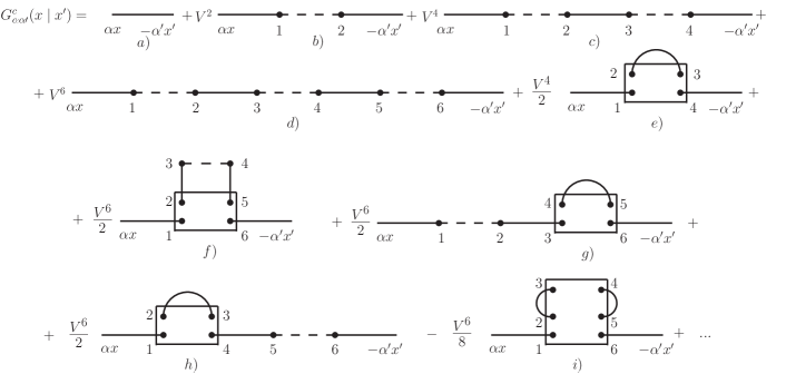
Figure 1: The first six orders of perturbation theory for conduction electron propagator. The solid and dashed thin lines depict zero order propagators for $c-$ and $f-$ electrons correspondingly. The rectangles depict the irreducible Green’s functions. The points of diagram are the vertices with $\alpha$ and $V$ contributions.

The contributions of the diagrams Fig. 1 b) and e) are the following

$$V^{2}\sum\limits_{\alpha_{1}\alpha_{2}}\sum\limits_{12}\alpha_{1}\alpha_{2}G_{\alpha\alpha_{1}}^{c(0)}(x|1)G_{\alpha_{1}\alpha_{2}}^{f(0)}(1|2)G_{\alpha_{2}\alpha^{\prime}}^{c(0)}(2|x^{\prime}),$$

$$\frac{V^{4}}{2}\sum\limits_{\alpha_{1}...\alpha_{4}}\sum\limits_{1...4}\alpha_{1}\alpha_{2}\alpha_{3}\alpha_{4}G_{\alpha\alpha_{1}}^{c(0)}(x|1)G_{\alpha_{2}\alpha_{3}}^{c(0)}(2|3)\times$$

$$\times G_{\alpha_{4}\alpha^{\prime}}^{c(0)}(4|x^{\prime})\left\langle Tf_{1}^{\alpha_{1}}f_{2}^{-\alpha_{2}}f_{3}^{\alpha_{3}}f_{4}^{-\alpha_{4}}\right\rangle_{0}^{ir}$$

correspondingly. It demonstrates the dependence of the diagrams from the charge quantum number $\alpha$.

The contributions of perturbation theory for $f-$ electron propagator are depicted on the Fig. 2

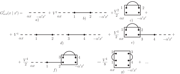
Figure 2: The contributions of the first four orders of perturbation theory for the $f-$ electron propagator.

The contributions of diagrams Fig. 2 b) and c) are equal to

$$V^{2}\sum\limits_{\alpha_{1}\alpha_{2}}\sum\limits_{12}\alpha_{1}\alpha_{2}G_{\alpha\alpha_{1}}^{f(0)}(x|1)G_{\alpha_{1}\alpha_{2}}^{c(0)}(1|2)G_{\alpha_{2}\alpha^{\prime}}^{f(0)}(2|x^{\prime}),$$

$$\frac{V^{2}}{2}\sum\limits_{\alpha_{1}\alpha_{2}}\sum\limits_{12}\alpha_{1}\alpha_{2}G_{\alpha_{1}\alpha_{2}}^{c(0)}(1|2)\left\langle Tf_{x}^{\alpha}f_{1}^{-\alpha_{1}}f_{2}^{\alpha_{2}}f_{x^{\prime}}^{-\alpha^{\prime}}\right\rangle_{0}^{ir},$$

correspondingly.

Between the diagrams for the one-particle $f-$ propagator there are strong and weak connected ones. The weak connected diagrams can be separated in two parts by cutting one propagator line. The sum of all strong connected diagrams for $f-$ electron belong to the correlation function which is denoted by us as $\Lambda_{\alpha\alpha^{\prime}}(x|x^{\prime})$ function. The quantity $\Lambda_{\alpha\alpha^{\prime}}(x|x^{\prime})$ is defined by the equation

$$\Lambda_{\alpha\alpha^{\prime}}(x|x^{\prime})=G_{\alpha\alpha^{\prime}}^{f(0)}(x|x^{\prime})+Z_{\alpha\alpha^{\prime}}(x|x^{\prime}),$$ (15)

where the function $Z_{\alpha\alpha^{\prime}}(x|x^{\prime})$ contains the contribution of strongly connected diagram based on the irreducible many-particle Green’s functions.

The strong connected part of the $c-$ electron propagator without the external lines is determined by us as a mass operator for uncorrelated electrons. This quantity is denoted as $\Sigma_{\alpha\alpha^{\prime}}(x|x^{\prime})$.

A simple relation exists between these two functions:

$$\Sigma_{\alpha\alpha^{\prime}}(x|x^{\prime})=V^{2}\alpha\alpha^{\prime}\Lambda_{\alpha\alpha^{\prime}}(x|x^{\prime})$$ (16)

The analysis of the propagator diagrams permits us to formulate the following Dyson equation for uncorrelated electron propagator

$$G_{\alpha\alpha^{\prime}}^{c}(x|x^{\prime}) = G_{\alpha\alpha^{\prime}}^{c(0)}(x|x^{\prime})+$$

$$+ \sum\limits_{\alpha_{1}\alpha_{2}}\sum\limits_{12}G_{\alpha\alpha_{1}}^{c(0)}(x|1)\Sigma_{\alpha_{1}\alpha_{2}}(1|2)G_{\alpha_{2}\alpha^{\prime}}^{c}(2|x^{\prime}).$$

At the same time we can formulate the Dyson-type equation for correlated electron propagator $G^{f}$:

$$G_{\alpha\alpha^{\prime}}^{f}(x|x^{\prime})=\Lambda_{\alpha\alpha^{\prime}}(x|x^{\prime})+$$ (18)

$$+V^{2}\sum\limits_{\alpha_{1}\alpha_{2}}\sum\limits_{12}\alpha_{1}\alpha_{2}\Lambda_{\alpha\alpha_{1}}(x|1)G_{\alpha_{1}\alpha_{2}}^{c(0)}(1|2)G_{\alpha_{2}\alpha^{\prime}}^{f}(2|x^{\prime}).$$

In equation (15) and (16) as in the previous equations which contain repeated indices $(1,2)$ is supposed summation by sites indices $(\mathbf{1},\mathbf{2})$, spin indices $(\sigma_{1},\sigma_{2})$ and integration by time variables $(\tau_{1},\tau_{2})$ in the interval $(0,\beta)$.

Unfortunate the Dyson-type equations far correlation function $\Lambda_{\alpha\alpha^{\prime}}$ and mass operator $\Sigma_{\alpha\alpha^{\prime}}$ don’t exist. Therefore the calculation of the $c-$ and $f-$ renormalized propagators needs the approximations based on the summation of special classes of diagrams.

On the Fig. 3 the skeleton diagrams for the correlation function $\Lambda_{\alpha\alpha^{\prime}}(x|x^{\prime})$ are depicted . They demonstrate impossibility to formulate Dyson-type equation for this function.

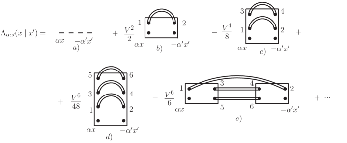
Figure 3: The skeleton diagrams for correlation function $\Lambda_{\alpha\alpha^{\prime}}(x|x^{\prime})$. The thin dashed line is zero-order $f-$ electron Green’s function. The rectangles depict the many-particles irreducible Green’s function. The double solid lines depict the renormalized conduction electron Green’s function $G_{\alpha\alpha^{\prime}}^{c}(x|x^{\prime})$.

The number of skeleton diagrams depicted on the Fig. 3 for the correlation function is infinite.

The contribution of the diagrams Fig. 3 b) and c) is the following:

$$\frac{1}{2}\sum\limits_{\alpha_{1}\alpha_{2}}\sum\limits_{12}\alpha_{1}\alpha_{2}G_{\alpha_{1}\alpha_{2}}^{c}(1|2)\left\langle Tf_{x}^{\alpha}f_{1}^{-\alpha_{1}}f_{2}^{\alpha_{2}}f_{x^{\prime}}^{-\alpha^{\prime}}\right\rangle_{0}^{ir},$$

$$-\frac{1}{8}\sum\limits_{\alpha_{1}...\alpha_{4}}\sum\limits_{1...4}\alpha_{1}\alpha_{2}\alpha_{3}\alpha_{4}G_{\alpha_{1}\alpha_{2}}^{c}(1|2)G_{\alpha_{3}\alpha_{4}}^{c}(3|4)\times$$

$$\times\left\langle Tf_{x}^{\alpha}f_{1}^{-\alpha_{1}}f_{2}^{\alpha_{2}}f_{3}^{-\alpha_{3}}f_{4}^{\alpha_{4}}f_{x^{\prime}}^{-\alpha^{\prime}}\right\rangle_{0}^{ir},$$

correspondingly.

If we take into account only the first term of the right-hand part of Fig. 3 we obtain the simplest Hubbard I approximation with consideration only of the chain-type diagrams.

The diagram Fig. 3 b) is the simplest contribution to correlation function which takes into account the electronic correlations. The diagrams Fig. 3 b), c) and d) are localized and their Fourier representations in real space are independent of momentum. There are also other diagrams of this kind with irreducible functions $G_{5}^{(0)ir},G_{6}^{(0)ir}$ and so on. The coefficients before these diagrams are determined by the number $\frac{1}{2^{n}n!}$, where $2n$ is the perturbation theory order of diagram. The last diagram of Fig. 3 is not local and its Fourier representation depends of the momentum. To dynamical mean field theory only the first group of local diagrams of Fig. 3 correspond.

The transition of the diagram contribution from superconducting version to the normal one is realized by the condition of equality to zero of the sums of all $\alpha-$ indices of every dynamical quantity. For example such transition of the diagram Fig. 3 b) is conditioned by the equalities $\alpha_{1}-\alpha_{2}=0$ and $\alpha-\alpha_{1}+\alpha_{2}-\alpha^{\prime}=0$ with solution $\alpha_{1}=\alpha_{2}$ and $\alpha=\alpha^{\prime}$.

The summation by $\alpha_{1}$ gives us two equal contributions and the coefficient before diagram increases twofold and becomes $1$ instead originally $\frac{1}{2}$.

In normal state the correlation function $\Lambda(x|x^{\prime})$ has a form depicted on the Fig. 4.

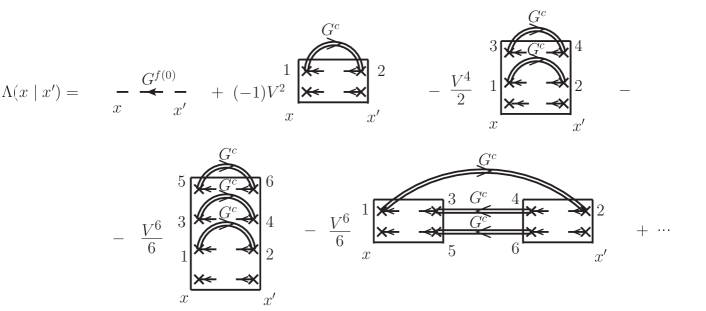
Figure 4: Correlation function $\Lambda(x|x^{\prime})$ in normal state. All the lines correspond to normal propagators and have a direction of propagators and of the arrays in the vertices.

The new coefficient before the diagrams take into account the existence of different possibilities of transition from superconducting to normal state.

After discussion of the propagators properties we shall proceed to the main part of our paper and investigate the properties of evolution operator average.

IV Vacuum diagrams

By using the perturbation theory we have obtained for the connected part of evolution operator average the contributions depicted in the Fig. 5.

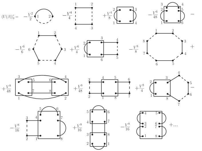
Figure 5: Vacuum diagrams of first eight orders of perturbation theory in superconducting state.

The contributions of the first, third and fourth diagrams of Fig. 5 are enumerated below:

$$-\frac{V^{2}}{2}\sum\limits_{\alpha_{1}\alpha_{2}}\sum\limits_{12}\alpha_{1}\alpha_{2}G_{\alpha_{1}\alpha_{2}}^{c(0)}(1|2)G_{\alpha_{2}\alpha_{1}}^{f(0)}(2|1),$$

$$\frac{V^{4}}{8}\sum\limits_{\alpha_{1}...\alpha_{4}}\sum\limits_{1...4}\alpha_{1}\alpha_{2}\alpha_{3}\alpha_{4}G_{\alpha_{1}\alpha_{2}}^{c(0)}(1|2)G_{\alpha_{3}\alpha_{4}}^{c(0)}(3|4)\times$$

$$\times\left\langle Tf_{1}^{-\alpha_{1}}f_{2}^{\alpha_{2}}f_{3}^{-\alpha_{3}}f_{4}^{\alpha_{4}}\right\rangle_{0}^{ir},$$

$$\ -\frac{V^{6}}{48}\sum\limits_{\alpha_{1}...\alpha_{6}}\sum\limits_{1...6}\alpha_{1}\alpha_{2}\alpha_{3}\alpha_{4}\alpha_{5}\alpha_{6}G_{\alpha_{1}\alpha_{2}}^{c(0)}(1|2)G_{\alpha_{3}\alpha_{4}}^{c(0)}(3|4)\times$$

$$\times G_{\alpha_{5}\alpha_{6}}^{c(0)}(5|6)\left\langle Tf_{1}^{-\alpha_{1}}f_{2}^{\alpha_{2}}f_{3}^{-\alpha_{3}}f_{4}^{\alpha_{4}}f_{5}^{-\alpha_{5}}f_{6}^{\alpha_{6}}\right\rangle_{0}^{ir}.$$

In normal state the diagrams of Fig. 5 are changed. The direction of propagator lines and of the arrays at vertices points appear together with new coefficients before the diagrams. This changing is demonstrated on the Fig. 6, where some of the diagrams of Fig. 5 are demonstrated.

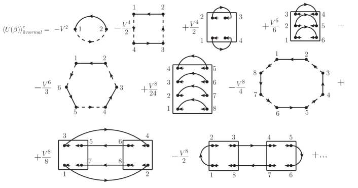
Figure 6: Some of the vacuum diagrams in normal state of the system.

Vacuum diagrams in superconducting and normal states contain the factor $\frac{1}{n}$, where $n$ is the order of perturbation theory in which given diagram appears. This factor makes difficult the investigation of this contributions. In order to remove this coefficient it is necessary to use the trick of integration by constant of interaction $V$. The result of such integration is depicted on the
Fig. 7.

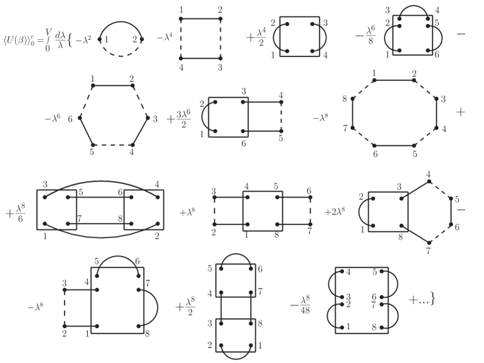
Figure 7: Vacuum diagrams of the system in superconducting state after integrating by interaction constant.

On the base of series expansions for renormalized propagators of the conduction $c-$ electrons (see Fig. 1), localized $f-$ electrons (see Fig. 2) and definition of the correlation function $\Lambda_{\alpha\alpha^{\prime}}(x|x^{\prime})$ we can prove that the contribution of the integrant of Fig. 7 in every order of perturbation theory can be presented itself as the product of some contribution from $G^{c}$ and some one from $\Lambda$. If the contribution of $G^{c}$ is of $n_{1}$ order of perturbation theory and of $\Lambda$ of $n_{2}$ order when the order of $\left\langle U(\beta)\right\rangle_{0}^{c}$ is equal to $n$ with the condition $n_{1}+n_{2}+2=n$ which must be satisfied. There are different possibilities to satisfy this condition and all of them must be taken into account.

For example there are three possibilities to compose from $G^{c}$ and $\Lambda$ the sixth diagrams of Fig. 7. These possibilities are enumerated below on the Fig. 8.

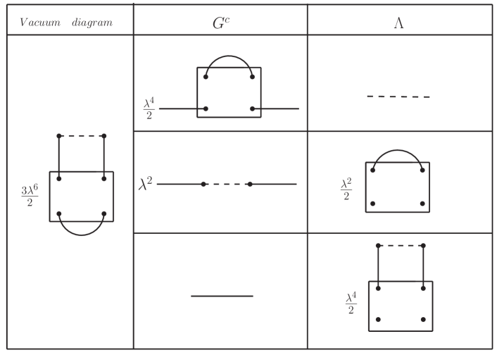
Figure 8: Three possibilities to organize the vacuum diagram of sixth order of perturbation theory. The correct coefficient $\frac{3}{2}$ is obtained by summing all the possibilities.

Other example of vacuum diagram of eighth order of perturbation theory is presented on the Fig. 9.

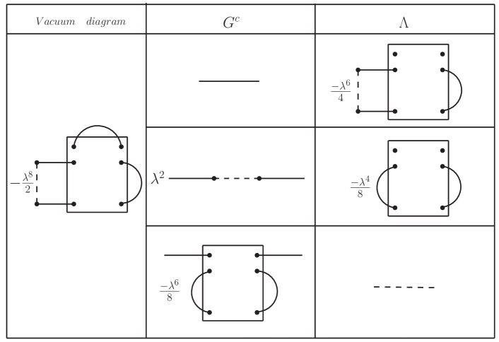
Figure 9: Three possibilities to obtain one of the vacuum diagram of eight order of perturbation theory.

Only all the three possibilities give us the correct coefficient $-\frac{1}{8}-\frac{1}{4}-\frac{1}{8}=-\frac{1}{2}$ of diagram. Other possibilities don’t exist. These examples demonstrate the general statement that the integrand of the evolution operator average can be presented itself as a product of $\lambda^{2}G^{c}\Lambda$ of the form

$$\left\langle U(\beta)\right\rangle_{0}^{c}=-\int\limits_{0}^{V}\frac{d\lambda}{\lambda}\sum\limits_{\alpha\alpha^{\prime}}\sum\limits_{xx^{\prime}}\alpha\alpha^{\prime}\lambda^{2}G_{\alpha\alpha^{\prime}}^{c}(x|x^{\prime}|\lambda)\Lambda{\alpha^{\prime}\alpha}(x^{\prime}|x|\lambda)=$$ (19)

$$=-\int\limits_{0}^{V}\frac{d\lambda}{\lambda}\sum\limits_{\alpha\alpha^{\prime}}\sum\limits_{xx^{\prime}}G_{\alpha\alpha^{\prime}}^{c}(x|x^{\prime}|\lambda)\Sigma{\alpha^{\prime}\alpha}(x^{\prime}|x|\lambda)=-\int\limits_{0}^{V}\frac{d\lambda}{\lambda}Tr(\hat{G}^{c}(\lambda)\hat{\Sigma}^{c}(\lambda)).$$

where the operators $\hat{G}^{c}(\lambda)$ and $\hat{\Sigma}^{c}(\lambda)$ have the matrix elements $G_{\alpha\alpha^{\prime}}^{c}(x|x^{\prime}|\lambda)$ and $\Sigma{\alpha\alpha^{\prime}}(x|x^{\prime}|\lambda)$ correspondingly. Index $\lambda$ underline that these quantities depend of the auxiliary constant of integration $\lambda$.

Therefore the thermodynamic potential of our system $F$ is equal to

$$F=F_{0}+\frac{1}{\beta}\int\limits_{0}^{V}\frac{d\lambda}{\lambda}Tr[\hat{G}^{c}(\lambda)\hat{\Sigma}^{c}(\lambda)].$$ (20)

This expression for renormalized thermodynamic potential of the strongly correlated system contains additional integration over the integration strength $\lambda$ and is awkward because it. Equation (18) generalizes the result of Luttinger and Ward ^[24] proved for non-correlated many-electron system in normal state.

Our generalization has been obtained for the case of strong correlations of special kind which contains one uncorrelated subsystem and one strongly correlated and we admit also the existence of superconductivity in both of them.

Luttinger and Ward have proved the possibility to transform this expression into much more convenient formula without such integration. For that they used a special functional constricted from skeleton diagrams the lines of which are the renormalized electron Green’s functions. We shall use the skeleton diagrams of strongly correlated system which differ essential from Luttinger and Ward ^[24] case and transform equation (18) to more convenient form.

In our strong correlated case we introduce the following functional

$$Y=-\frac{1}{2\beta}Tr{\{\ln(\hat{G}^{c(0)}\hat{\Sigma}-1)+\hat{G}^{c}\hat{\Sigma}}\}+Y^{\prime},$$ (21)

which is the generalization of the Luttinger-Ward ^[24] equation just for the strongly correlated systems. Here operation $Tr$ use the summation by $\alpha,\sigma,\mathbf{i}$ and integration by $\tau$.

The quantity $Y^{\prime}$ contains all peculiarities of the strongly correlated systems and is presented itself as a sum of closed linked skeleton diagrams, constructed from irreducible Green’s functions of correlated electrons and full Green’s functions of uncorrelated electrons.

On the Fig. 10 are depicted some of simplest skeleton diagrams for functional $Y^{\prime}$. These diagrams depend of the interaction strength $V$ not only through the factors in the front of each diagram but also through the dependence of full Green’s function $G^{c}(V)$.

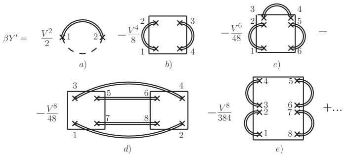
Figure 10: Skeleton diagrams for functional $Y^{\prime}$.

The contributions of the diagrams a), b) and c) are following

$$\frac{V^{2}}{2}\sum\limits_{\alpha_{1}\alpha_{2}}\sum\limits_{12}\alpha_{1}\alpha_{2}G_{\alpha_{1}\alpha_{2}}^{f(0)}(1,2|V)G_{\alpha_{2}\alpha_{1}}^{c}(2,1|V),$$

$$-\frac{V^{4}}{8}\sum\limits_{\alpha_{1}...\alpha_{4}}\sum\limits_{1...4}\alpha_{1}\alpha_{2}\alpha_{3}\alpha_{4}G_{\alpha_{1}\alpha_{2}}^{c}(1,2|V)G_{\alpha_{3}\alpha_{4}}^{c}(3,4|V)\times$$

$$\times\left\langle Tf_{1}^{-\alpha_{1}}f_{2}^{\alpha_{2}}f_{3}^{-\alpha_{3}}f_{4}^{\alpha_{4}}\right\rangle_{0}^{ir},$$

$$\ \frac{V^{6}}{48}\sum\limits_{\alpha_{1}...\alpha_{6}}\sum\limits_{1...6}\alpha_{1}\alpha_{2}\alpha_{3}\alpha_{4}\alpha_{5}\alpha_{6}G_{\alpha_{1}\alpha_{2}}^{c}(1,2|V)G_{\alpha_{3}\alpha_{4}}^{c}(3,4|V)\times$$

$$\times G_{\alpha_{5}\alpha_{6}}^{c}(5,6|V)\left\langle Tf_{1}^{-\alpha_{1}}f_{2}^{\alpha_{2}}f_{3}^{-\alpha_{3}}f_{4}^{\alpha_{4}}f_{5}^{-\alpha_{5}}f_{6}^{\alpha_{6}}\right\rangle_{0}^{ir}.$$

From Fig. 3 and Fig. 10 it is possible to demonstrate the following equation:

$$\frac{\delta\beta Y^{\prime}}{\delta G_{\alpha_{1}\alpha_{2}}(1,2)}=\frac{\alpha_{1}\alpha_{2}}{2}V^{2}\Lambda_{\alpha_{2}\alpha_{1}}(2,1)=\frac{1}{2}\Sigma_{\alpha_{2}\alpha_{1}}(2,1).$$ (22)

If we take into account only the explicit dependence of the functional $Y^{\prime}$ of interaction constant $V$ without considering the dependence of the full Green’s functions $G^{c}(V)$ from $V$ we shall obtain the other property:

$$V\beta\frac{dY^{\prime}}{dV}\mid_{G^{c}}=\sum\limits_{\alpha_{1}\alpha_{2}}\sum\limits_{12}G_{\alpha_{1}\alpha_{2}}^{c}(2,1|V)\Sigma_{\alpha_{1}\alpha_{2}}(1,2|V)=\\ Tr[\hat{\Sigma}\hat{G}^{c}].$$

Because of the necessity to have the functional derivatives over mass operator $\Sigma$ we shall use the Dyson equation (15) rewritten in the form $[x=(\alpha,\mathbf{x},\sigma,\tau)]$:

$$G^{c(0)-1}(x,x^{\prime})=G^{c-1}(x,x^{\prime})+\Sigma(x,x^{\prime})$$ (23)

We obtain

$$\frac{\delta G^{c}(x,x^{\prime})}{\delta\Sigma(y,y^{\prime})}=G^{c}(x,y)G^{c}(y^{\prime},x^{\prime}),$$ (24)

and

$$\frac{\delta}{\delta\Sigma(y,y^{\prime})}Tr\ln(1-\hat{G}^{c(0)}\hat{\Sigma})=-G^{c}(y^{\prime},y),$$

$$\frac{\delta}{\delta\Sigma(y,y^{\prime})}Tr(\hat{G}^{c}\hat{\Sigma})=G^{c}(y^{\prime},y)+(\hat{G}^{c}\hat{\Sigma}\hat{G}^{c})_{y^{\prime}y}$$ (25)

By summing these equations we obtain:

$$\frac{\delta}{\delta\Sigma(y,y^{\prime})}(-\frac{1}{2\beta})Tr{\{\ln(\hat{G}^{c(0)}\hat{\Sigma}-1)+\hat{G}^{c}\hat{\Sigma}}\}=$$

$$=-\frac{1}{2\beta}(\hat{G}^{c}\hat{\Sigma}\hat{G}^{c})_{y^{\prime}y}.$$ (26)

On the base of definition of the functional $Y^{\prime}$ Fig. 10 and equation (20) we have

$$\frac{\delta Y^{\prime}}{\delta\Sigma(y,y^{\prime})}=\sum\limits_{xx^{\prime}}\frac{\delta Y^{\prime}}{\delta G^{c}(x,x^{\prime})}\frac{\delta G^{c}(x,x^{\prime})}{\delta\Sigma(y,y^{\prime})}=\frac{1}{2\beta}(\hat{G}^{c}\hat{\Sigma}\hat{G}^{c})_{y^{\prime}y}.$$ (27)

As a result we obtain the stationarity property of the functional $Y$:

$$\frac{\delta Y}{\delta\Sigma(y,y^{\prime})}=0.$$ (28)

Now we shall discuss the derivative over interaction constant $V$ of functional $Y$. We shall taken into account the stationarity $Y$ about $\hat{\Sigma}$ and $\hat{G}^{c}$ and equation (21). We obtain:

$$V\frac{dY}{dV}=V\frac{\partial Y}{\partial V}\mid_{\Sigma}+V\frac{\delta Y}{\delta\Sigma}\frac{\partial\Sigma}{\partial V}=V\frac{\partial Y^{\prime}}{\partial V}\mid_{\Sigma}=\frac{Tr(\hat{\Sigma}\hat{G}^{c})}{\beta}.$$ (29)

From equation (18) we have:

$$V\frac{dF}{dV}=\frac{Tr(\hat{G}^{c}\hat{\Sigma})}{\beta},$$ (30)

and as a consequence we establish

$$V\frac{dF}{dV}=V\frac{dY}{dV},$$ (31)

with the solution

$$F=Y+\textsc{const}.$$

This constant is $F_{0}$. Therefore

$$F=F_{0}+Y,$$

with the stationary property

$$\frac{\delta F}{\delta\Sigma(x,x^{\prime})}=0,$$ (32)

as in superconducting and in normal states.

V Heat Capacity [25]

As a illustration of our results we shall consider the problem of finding the heat capacity of our strongly correlated system in normal state and at the low temperatures.

The heat capacity at constant volume $V$ is equal to

$$C_{V}=T(\frac{\partial S}{\partial T})_{V},$$

where the entropy $S$ is given by

$$S=-T(\frac{\partial F}{\partial T})_{\mu,V}.$$

The quantity $\mu$ is the chemical potential at temperature $T$.

At low temperature we may expand $F(\mu,V,T)$ and $\mu$ in even powers of the temperature:

$$F = F(\mu_{0},V,0)-\frac{1}{2}\gamma(\mu_{0},V)T^{2}+...,$$

$$\mu(T) = \mu_{0}+\mu^{\prime}T^{2}+...,$$

where $\mu_{0}$ is the value of chemical potential for correlated system at $T=0$.

As a result we have

$$C_{V}=\gamma(\mu_{0},V)T+...$$

the linear dependence of the heat capacity of the temperature at low its values. Therefore to evaluate the coefficient $\gamma(\mu_{0},V)$ it is necessary to obtain the expansion of $F$ in powers of $T$ by using the expression (31), (19) and Fig.10 for $Y^{\prime}$ obtained by us in previous part of the paper.

We know that the expression (19) for $Y$ and (31) for thermodynamic potential is stationary with respect to changes in the proper self-energy $\Sigma_{\mathbf{k}}(i\omega_{0}).$ Therefore because we are interested in the first corrections to $F$, we can neglect the explicit temperature dependence of mass operator $\Sigma(\mathbf{k}|i\omega)$ and $G^{c}(\mathbf{k}|i\omega)$ and replace them by values $\Sigma(\mathbf{k}|i\omega_{0})|_{T=0}$ and $G^{c}(\mathbf{k}|i\omega_{0})|_{T=0}$ calculated at $T=0$. Thus the first correction to the $T=0$ value of $F$ (31) comes only from the difference between the $\omega_{n}$ sums in expression (31) and what we would get if we replace them by integrals according to the equation

$$\frac{1}{\beta}\sum\limits_{\omega_{n}}=\frac{1}{2\pi}\int\limits_{-\infty}\limits^{\infty}d\omega.$$

Now it is necessary to consider the functional $Y^{\prime}$ on Fig.10. Since each line of a skeleton diagram of functional $Y^{\prime}$ contains an $\omega_{n}$ sum, the total first correction to $Y^{\prime}$ is obtained by correcting the computation in each diagram for a single line and use equation (37) for the other $\omega_{n}$ sums of the diagram, finally summing over every line.

In such a way we obtain the contribution of one line of skeleton diagram multiplied by the number of lines of skeleton diagrams. This number changes the coefficient before the skeleton diagram of $Y^{\prime}$ and new coefficients correspond to new contribution to $Y^{\prime}$ equal to the self-energy one. This quantity has the form of second term in right hand part of functional (19) for $Y$ having the opposite sign. When we combine the both part of functional $Y$ these quantities are reciprocally canceled.

Finally we obtain to the first order for $F$ the equation

$$F = F_{0}-\frac{1}{2\beta}\sum\limits_{\sigma\mathbf{k}}\sum\limits_{\omega_{n}}\ln[G^{c(0)}(i\omega_{n})\Sigma(\mathbf{k}|i\omega_{n})|_{T=0}-1]e^{i\omega_{n}0^{+}}=$$

$$= F_{0}+\frac{1}{2\beta}\sum\limits_{\sigma\mathbf{k}}\sum\limits_{\omega_{n}}\ln[i\omega_{n}-\epsilon_{\mathbf{k}}]e^{i\omega_{n}0^{+}}-\frac{1}{2\beta}\sum\limits_{\sigma\mathbf{k}}\sum\limits_{\omega_{n}}\ln[\Sigma(\mathbf{k}|i\omega_{n})|_{T=0}-(G^{c(0)}(i\omega_{n}))^{-1}]e^{i\omega_{n}0^{+}}.$$

We use the Poisson equation for the $\omega_{n}$ sums and write them as an integral

$$F = F_{0}-\frac{1}{2}\sum\limits_{\sigma\mathbf{k}}\int\limits_{C}\frac{dze^{z0^{+}}}{e^{\beta z}+1}ln[G^{c(0)}(z)\Sigma(\mathbf{k}|z)|_{T=0}-1],$$ (34)

where $C$ is contour which surrounds in anti clock wise direction the poles of the function $(e^{\beta z}+1)^{-1}$ in the points $z=i\omega_{n}=\frac{(2n+1)\pi}{\beta}i$. The term in last equation proportional to $T^{2}$ is obtained by usual Sommerfeld technique.

The details of such computation will be discussed in other place.

VI Conclusions

We have developed the diagrammatic theory for PAM on the base of new conceptions proposed by us for strongly correlated electron systems.

We introduced the notion of correlation function $\Lambda_{\alpha\alpha^{\prime}}(x|x^{\prime})$ of $f-$ electrons (see Fig. 3) which is the infinite sum of strong connected irreducible Green’s functions and which contains the most important spin, charge and pairing fluctuations of the correlated $f-$ electrons. This correlation function determines the mass operator $\Sigma_{\alpha\alpha^{\prime}}(x|x^{\prime})$ (14) of the uncorrelated conduction electrons. The both these quantities $\Lambda$ and $\Sigma$ permit us to formulate the Dyson equation for $c-$ electrons (15) and Dyson-type equation (16) for $f-$ electrons. These results are expressed in general form appropriate as for normal and as for superconducting state.

We have obtained the skeleton diagrams for $\Lambda$ function and demonstrated their dependence from irreducible many-particle Green’s functions $G_{n}^{(0)ir}(1,...,2n)$ with all values of $n$ and also of $c-$ electrons full propagators. Thanks the presence of these irreducible Green’s functions it is impossible to formulate Dyson-type equations for $\Lambda$ and $\Sigma$ quantities.

The results are appropriate as for normal and as the superconducting state. Unification of the investigation for the both phases was possible thanks the introducing of the notion of quantum charge number $\alpha$ and the rewritten of the interaction Hamiltonian in such new form.

From Fig. 3 it is clear that the simplest contribution that takes into account $f-$ electron correlations is reduced to first two terms of right-hand part of this figure. All the terms of Fig. 3 besides the last one and also other omitted diagrams like them are local with Fourier representation independent of momentum. These terms correspond to the structure of dynamical mean field theory. Last diagram of Fig. 3 and other more complicated diagrams with more number of irreducible Green’s functions depend of momentum and take in consideration of the space fluctuations. The local contributions take into account only of the fluctuations in time.

We have demonstrated the transition of our diagram from superconducting to normal state by using the additional conditions imposed on the charge quantum numbers of which depend the dynamical quantities.

The special investigation of vacuum diagram has been done after introducing the auxiliary interaction strength and integration by it of these diagram contributions. We have proved that this integrant is equal to the product of two matrices $\Sigma_{\alpha\alpha^{\prime}}$ and $G_{\alpha\alpha^{\prime}}^{c}$.

Then we have introduced special functional in the form of skeleton diagrams and proved it coincidence with thermodynamical potential. This expression has the property of stationary relative the changing of the mass operator or full Green’s function $G^{c}$ of conduction electrons.

References

• (1) P. W. Anderson, Phys. Rev. 124, 41 (1961).
• (2) H. Reiter and G. Morandi, Phys. Rep. 143, 277 (1984).
• (3) G. Czycholl, Phys. Rep. 143, 277 (1986).
• (4) D. M. Newns and N. Read, Adv. Phys. 36, 799 (1987).
• (5) H. Shiba and P. Fazekas, Prog. Theor. Phys. Suppl. 101, 403 (1990).
• (6) Canio Noce, Phys. Rep. 431, 173 (2006).
• (7) P. Fulde, J. Keller and G. Zwicknagl, Solid State Phys. 41, 2 (1988).
• (8) A. C. Hewson , The Kondo Problem to Heavy Fermions, Cambridge University Press, Cambridge, England (1993).
• (9) P. Fulde, Electron correlations in Molecules and Solids, Springer, Berlin (1991) .
• (10) M. I. Vladimir and V. A. Moskalenko, Theor. Math. Phys. 82, 301 (1990).
• (11) S. I. Vakaru, M. I. Vladimir and V. A. Moskalenko, Theor. Math. Phys. 85, 1185 (1990).
• (12) N. N. Bogoliubov and V. A. Moskalenko, Theor. Math. Phys. 80, 10 (1991).
• (13) N. N. Bogoliubov and V. A. Moskalenko, Theor. Math. Phys. 92, 820 (1992).
• (14) V. A. Moskalenko, Theor. Math. Phys. 110, 243 (1997); Teor. Mat. Fiz. 110, 308 (1997).
• (15) V. A. Moskalenko, Theor. Math. Phys. 116, 1094 (1998); Teor. Mat. Fiz. 116, 456 (1998).
• (16) V. A. Moskalenko, P. Entel, D. F. Digor, L. A. Dohotaru
and R. Citro, Theor. Math. Phys. 155, 535 (2008); Teor. Mat. Fiz. 155, 914 (2008).
• (17) V. A. Moskalenko, P. Entel, L. A. Dohotaru, D. F. Digor
and R. Citro, Diagrammatic theory for Anderson Impurity Model, Preprint JINR, Dubna, E17-2008-56.
• (18) V. A. Moskalenko, P. Entel, L. A. Dohotaru
and R. Citro, Theor. Math. Phys. 159, 454 (2009); Teor. Mat. Fiz. 159, 500 (2009).
• (19) V. A. Moskalenko, P. Entel and D. F. Digor, Phys. Rev. B 59, 619 (1999).
• (20) V. A. Moskalenko, P. Entel, M. Marinaro, N. B. Perkins and C. Holfort, Phys. Rev. B 63, 245119 (2001).
• (21) J. Hubbard, Proc. Roy. Soc. A276, 238 (1963), A281, 401 (1964), A285, 542 (1965).
• (22) A. A. Abrikosov, L.P.Gor’kov and I. E. Dzyaloshinsky, The method of quantum field theory in statistical physics, Dobrosvet, Moscow (1998).
• (23) N. N. Bogoliubov, Full collection of papers, Vol. 10, Moscow, Nauka, (2007).
• (24) J. M. Luttinger and J. C. Ward, Phys. Rev. 118, N5, 1417 (1960).
• (25) J. M. Luttinger, Phys. Rev. 119, 1153 (1960).