Abstract

Using non-relativistic effective field theory in 1+1 dimensions, we generalize Lüscher’s approach for resonances in the presence of an external field. This generalized approach provides a framework to study the infinite-volume limit of the form factor of a resonance determined in lattice simulations.

Pacs:		11.15.Ha, 12.38.Gc, 11.10.St
Keywords:		Lattice field theory, resonances, finite volume, Lüscher formula, magnetic moment

1 Introduction

Recently, the external field method has been widely used to calculate magnetic moments and polarizabilities of both stable and excited hadrons in lattice QCD [1, 2, 3, 4, 5, 6, 7, 8]. In an alternative approach, the three-point function, evaluated in lattice QCD, is extrapolated in the photon momentum squared variable $q^{2}$ to the value $q^{2}=0$ (see, e.g., [9, 10]). Both methods are justified in case of stable particles. In case of excited hadron states, however, conceptual problems arise. As it is well known, resonances are not described by a single level in the spectrum of the Hamiltonian. Rather, they characterize the whole spectrum and are usually extracted by applying Lüscher’s formula to the lattice data at different lattice volumes [11]. In order to proceed with the determination of, e.g. the magnetic moment of a resonance, the generalization of Lüscher’s approach in the presence of external fields is needed. For example, it is not clear, how the real and discrete energy eigenvalues of a system, placed in an external field, are related to the resonance form factor, which is a complex quantity in general. To the best of our knowledge, such a generalization is not available at present and we will fill this gap in the following.

In order to extract the form factors of resonances on the lattice, one has to thoroughly study the volume dependence of these quantities. As it is well known, non-relativistic effective field theories (NR EFTs) provide the most convenient framework to systematically address this problem. In the past such kind of theories have been used to obtain a simple derivation of Lüscher’s formula [12], including the cases of particles with spin [13] and multi-channel scattering [14]. Moreover, EFT techniques have been applied to the calculation of the volume dependence of the meson and nucleon form factors [15, 16, 17]. In this paper, using an effective field theory in 1+1 dimensions, we discuss the generalization of Lüscher’s approach in the presence of an external field. The outline of the procedure is as follows. We first assume that, in the absence of the external field, the standard effective-range expansion converges in a part of the complex momentum plane including the (complex) resonance pole denoted by $p_{*}$. This fact can be used to perform the analytic continuation of Lüscher’s formula and to find the position of the pole. The key observation is that the limit $p\to p_{*}$ in Lüscher’s formula corresponds to the infinite-volume limit. In turn, this leads to the conclusion that the shift of the pole position in the external field, evaluated at lowest order in this field, is proportional to the resonance form factor evaluated in the infinite volume and on the mass shell $p\to p_{*}$.

The situation in 3+1 dimensions is different from 1+1 dimensions in one important aspect. Namely, whereas in 1+1 dimensions the limit $p\to p_{*}$ always implies the infinite-volume limit, we expect that there are in addition what we term as finite fixed points in 3+1 dimensions. Owing to this fact, together with some additional technical complications which arise in the 3+1-dimensional case, we find it convenient to separate these two cases. In the present paper, we limit ourselves to a toy model of a resonance in an external field in 1+1 dimensions. The 3+1-dimensional case will be addressed in future publications.

The outline of the paper is as follows. In section 2 we construct the non-relativistic effective theory, introducing the resonance field as an independent degree of freedom. Fixing the pole position in the two-point function of the resonance field in the complex plane is discussed. Turning on the external field and the resulting shift of the pole position is considered in section 3. The relation of the mass-shell limit $p\to p_{*}$ and the infinite-volume limit is discussed in section 4. In section 5 we address the evaluation of the three-point function related to the form factor under consideration. Section 6 contains our conclusions. Finally, the calculation of the loop function in the infinite and in a finite volume is relegated to the appendix A.

2 Non-relativistic field theory in the absence of an external field

Below, we shall use the “relativized” version of NR EFT, which has been first introduced in Ref. [18]. The theory in a finite volume was first considered in Refs. [13, 14]. For all details, we refer the interested reader to these articles. Here, we consider two massive scalar non-relativistic fields $\Psi$ and $\Phi$ in 1+1 dimensions. The non-relativistic Lagrangian that describes these particles is given by

$${\cal L} = \Psi^{\dagger}\left(i\partial_{t}-w_{\Psi}(\nabla^{2})\right)2w_{\Psi}(\nabla^{2})\Psi+\Phi^{\dagger}\left(i\partial_{t}-w_{\Phi}(\nabla^{2})\right)2w_{\Phi}(\nabla^{2})\Phi$$ (1)

$$+ C_{0}\Psi^{\dagger}\Phi^{\dagger}\Phi\Psi+C_{1}\biggl{\{}(\Psi^{\dagger}\stackrel{{\scriptstyle\leftrightarrow}}{{\nabla^{2}}}\Phi^{\dagger})\,\Phi\Psi+\text{h.c.}\biggr{\}}+\cdots\,,$$

where $w_{i}(\nabla^{2})\doteq(m_{i}^{2}-\nabla^{2})^{1/2}$ for $i=\Psi,\Phi$, and $(u\!\stackrel{{\scriptstyle\leftrightarrow}}{{\nabla^{2}}}\!v)\doteq u\nabla^{2}v+v\nabla^{2}u$. The low-energy constants $C_{0},C_{1},\ldots$ are related to the effective-range expansion of the $\Psi\Phi$ elastic scattering amplitude and the ellipses stand for the terms with higher derivatives. At tree level, this scattering amplitude in the center-of-mass frame is given by the expression

$$H(p,q)=C_{0}-2C_{1}(p^{2}+q^{2})+\cdots\,,$$ (2)

where $p,q$ denote the relative momenta of the $\Psi\Phi$-pair in the final and initial state, respectively.

In the non-relativistic field theory, the full scattering amplitude $T(p,q)$ is obtained by summing up the tree-level result given in Eq. (2) to all orders. The result for the on-shell amplitude in the CM frame is given by

$$T(p,p)=\frac{H(p,p)}{1-J(p)H(p,p)}\,,$$ (3)

where $J(p)$ denotes the $\Psi\Phi$-loop integral, evaluated by expanding the integrand in powers of momenta and using dimensional regularization (see Ref. [18] and Appendix A for more details), in the center-of-mass frame we obtain

$$J(p) = \int\frac{d^{D}k}{(2\pi)^{D}i}\frac{1}{2w_{\Psi}(k)2w_{\Phi}(k)}\frac{1}{\left(w_{\Psi}(k)-P^{0}+k^{0}\right)\left(w_{\Phi}(k)-k^{0}\right)}$$ (4)

$$= \frac{i}{4P^{0}p}+O(D-2)\,,$$

where $P^{0}=w_{\Psi}(p)+w_{\Phi}(p)$ is the center-of-mass energy of the $\Psi\Phi$ system, and $p$ stands for the relative momentum of the $\Psi\Phi$-pair.

The unitarity relation is

$$\mbox{Im}\,T(p,p)=\frac{1}{4P^{0}p}\,|T(p,p)|^{2}\,,\quad\quad T(p,p)=\frac{4P^{0}p}{\cot\,\delta(p)-i}\,,$$ (5)

where $\delta(p)$ is the scattering phase. Comparing Eqs. (3) and (5), we obtain

$$p\cot\delta(p)=\frac{4P^{0}p^{2}}{H(p,p)}=A_{1}p^{2}+A_{2}p^{4}+\cdots\,,$$ (6)

where the effective range expansion parameters $A_{1},A_{2}\ldots$ can be expressed in terms of the effective couplings $C_{0},C_{1},\ldots$, see Eq. (2). Eq. (6) implies that the quantity $p\cot\delta(p)$ is an analytic function of the variable $p^{2}$ in the region of small $p^{2}$, where the effective range expansion converges. If there is a low-lying resonance in the $\Psi\Phi$ elastic scattering, the amplitude will have a pole on the second Riemann sheet. The pole position $p_{*}$ is determined by the equation $p_{*}\cot\delta(p_{*})=-ip_{*}$, where the analytic continuation to complex values of $p^{2}$ is performed by using the effective-range expansion displayed in Eq. (6) .

Suppose there is a low-lying resonance in $\Psi\Phi$ elastic scattering. In this case, it is convenient to use the equivalent formulation of the non-relativistic effective field theory, introducing an auxiliary “resonance field” $\chi$. The Lagrangian of this theory is given by

$${\cal L}_{\chi} = \Psi^{\dagger}\left(i\partial_{t}-w_{\Psi}(\nabla^{2})\right)2w_{\Psi}(\nabla^{2})\Psi+\Phi^{\dagger}\left(i\partial_{t}-w_{\Phi}(\nabla^{2})\right)2w_{\Phi}(\nabla^{2})\Phi$$ (7)

$$+ \chi^{\dagger}\left(i\partial_{t}-w_{\chi}(\nabla^{2})\right)2w_{\chi}(\nabla^{2})\chi+f_{0}\left(\Psi^{\dagger}\Phi^{\dagger}\chi+\text{h.c.}\right)$$

$$+ f_{1}\left((\Psi^{\dagger}\stackrel{{\scriptstyle\leftrightarrow}}{{\nabla^{2}}}\Phi^{\dagger})\chi+\text{h.c.}\right)\cdots\,,$$

where $f_{0},f_{1},\ldots$ are the low-energy couplings and $m_{\chi}$ in $w_{\chi}(\nabla^{2})=(m_{\chi}^{2}-\nabla^{2})^{1/2}$ is a real parameter. Note that we opted for elimination the 4-point vertices with $\Psi$ and $\Phi$ fields in the Lagrangian. Since the ultraviolet divergences do not emerge in the dimensional regularization, such 4-particle vertices are not generated by the loops either.

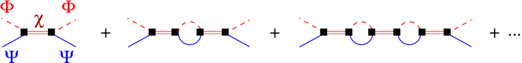
Figure 1: The $\Psi\Phi$ elastic scattering amplitude in the theory described by the Lagrangian ${\cal L}_{\chi}$ given in Eq. (7). Solid, dashed and double lines denote the $\Psi,\Phi$ and $\chi$ fields, respectively. The shaded squares denote the full three-particle vertex $\gamma(p)$.

The $\Psi\Phi$ elastic scattering amplitude in this framework is generated by summing up the bubble diagrams shown in Fig. 1

$$T(p,p)=\gamma^{2}(p)S_{\chi}(p)\,,\quad\quad S_{\chi}(p)=\frac{1}{2m_{\chi}(m_{\chi}-P^{0})-\Sigma_{0}(P^{0})}\,,$$ (8)

where $S_{\chi}$ stands for the propagator of the $\chi$ particle, $\Sigma_{0}(P^{0})=\gamma^{2}(p)J(p)$ is the self-energy of the field $\chi$, and

$$\gamma(p)=f_{0}-2f_{1}p^{2}+\ldots$$ (9)

denotes the full $\Psi\Phi\chi$ vertex function.

Comparing Eqs. (3) and (8) gives the matching between the two equivalent formulations

$$H^{-1}(p,p)=\frac{2m_{\chi}(m_{\chi}-P^{0})}{\gamma^{2}(p)}\,.$$ (10)

Further, the relation between the couplings $C_{i}$ and $f_{i}$ can be obtained by expanding both sides of the above equation in powers of $p^{2}$. In case when the low-lying resonance is present, the couplings $f_{i}$ are of natural size, whereas the couplings $C_{i}$ contain powers of the small scale $\Delta_{0}=m_{\chi}-m_{\Psi}-m_{\Phi}$ in the denominator and may become unnaturally large. The position of the resonance pole is given by

$$\frac{8m_{\chi}P^{0}_{*}p_{*}^{2}(m_{\chi}-P^{0}_{*})}{\gamma^{2}(p_{*})}=-ip_{*}\,,$$ (11)

where $P^{0}_{*}=w_{\Psi}(p_{*})+w_{\Phi}(p_{*})$.

In order to obtain the energy spectrum of the system described by the Lagrangian (7), placed in a box of size $L$, we consider the finite-volume propagator of the particle $\chi$

$$S^{L}_{\chi}(p)=\frac{1}{2m_{\chi}(m_{\chi}-P^{0})-\gamma^{2}(p)J^{L}(p)}\,,$$ (12)

where

$$J^{L}(p)=\frac{1}{L}\,\sum_{k}\int\frac{dk^{0}}{2\pi i}\frac{1}{2w_{\Psi}(k)2w_{\Phi}(k)}\frac{1}{\left(w_{\Psi}(k)-P^{0}+k^{0}\right)\left(w_{\Phi}(k)-k^{0}\right)}\,,$$

and $k$ denotes the discrete lattice momenta $k=2\pi n/L\,,\,\,n\in\mathbb{Z}$.

It can be shown (see Appendix A) that, up to the terms that vanish exponentially with $L$, the function $J^{L}(p)$ is given by

$$J^{L}(p)=-\frac{1}{4P^{0}p}\,\cot\,\frac{pL}{2}\,.$$ (14)

Using Eqs. (6), (10) and (14), it can be shown that the denominator in Eq. (12) vanishes for the values of $p$ which obey the relation $\cot\,\delta(p)=-\cot\,(\frac{1}{2}\,pL)$. This leads to the Lüscher equation [11] in 1+1 dimensions (we take the positive root $p>0$)

$$2\delta(p)=-pL+2\pi m\,,\quad\quad m\in\mathbb{N}\,.$$ (15)

Let us restrict ourselves to a fixed energy level ($m$ fixed) and measure $p_{m}=p_{m}(L)$ for different values of $L$ on the lattice. Substituting this into Lüscher’s equation, we get

$$p\,\cot\,\delta_{m}(p)=-p\,\cot\,(\frac{1}{2}\,pL_{m}(p))\,,$$ (16)

where the function $L=L_{m}(p)$ is the inverse of $p=p_{m}(L)$ and the index $m$ attached to the scattering phase indicates that it has been determined from the fixed level $m$.

The left-hand side of Eq. (16) is a function of the variable $p$ only. Fitting this function, extracted from the lattice measurement, to the effective range expansion in Eq. (6), one may determine the real coefficients $A_{1}^{m},A_{2}^{m},\ldots$ (the index $m$ again indicates the fixed energy level). If the volume $L$ is large enough (as required in the derivation of Lüscher’s equation), these coefficients do indeed not depend on the index $m$, up to exponentially suppressed terms.

Finally, assuming that the effective range expansion is convergent in the range of $p^{2}$ we are working, one may solve the equation $A_{1}p_{*}^{2}+A_{2}p_{*}^{4}+\ldots=-ip_{*}$ to obtain the complex pole position on the second Riemann sheet. The pole position remains stable up to exponentially suppressed terms (for this reason, we suppress the index $m$ in the quantities $A_{i}$ here).

Suppose now that we consider the limit $p\to p_{*}$ in Eq. (16), which we rewrite in the following form (the index $m$ is suppressed)

$$\cot\,\delta(p)=\frac{A_{1}p^{2}+A_{2}p^{4}\cdots}{p}=-\cot\,\pi q\,,\quad\quad q=\frac{pL(p)}{2\pi}~{},$$ (17)

where the known coefficients $A_{1},A_{2},\ldots$ are assumed to be extracted from lattice measurements at real values of $p$. At the pole position $p\to p_{*}$, the left-hand side of Eq. (17) tends to $-i$. Then, as it can be easily seen, $\text{Im}\,q\to-\infty$. The real part of the variable $q$ stays finite in this limit and depends on the path along which the pole $p_{*}$ is approached. The real and imaginary parts of the “volume” $L(p)$, defined by Eq. (17), also diverge in this limit.

The above observation plays the central role in study of the properties of a resonance in the external field. Loosely spoken, it states that the mass-shell limit for a resonance implies the infinite-volume limit. For this reason, e.g. the shift of the resonance pole position in an external field is determined by the vertex function at zero momentum transfer, calculated in the infinite volume.

3 Turning on the external field

In order to study the behavior of the system placed in an external field, one has to equip the Lagrangian with that field. Instead of introducing an electromagnetic field in two dimensions, we consider a toy model with a constant scalar external field $v$. To ease the notation, we in addition assume that the field $v$ does not couple to $\Phi$.

The modified Lagrangian takes the form

$${\cal L}^{v}_{\chi}={\cal L}_{\chi}+v\biggl{(}\Psi^{\dagger}\Psi+\lambda_{1}\chi^{\dagger}\chi+\lambda_{2}(\Psi^{\dagger}\Phi^{\dagger}\chi+\text{h.c.})\biggr{)}\,,$$ (18)

where the couplings $\lambda_{i}$ are dimensionless, It should be pointed out that, since the UV divergences are absent in dimensional regularization, the terms with derivatives acting on the fields, are not generated by loop corrections. Hence, one may omit these altogether without loss of generality.

Let us first restrict ourselves to the infinite volume. In the presence of the external field, the pole position in the two-particle function of the field $\Psi$ shifts from $P^{0}=(m_{\Psi}^{2}+p^{2})^{1/2}$ to $P^{0}=(m_{\Psi}^{2}-v+p^{2})^{1/2}+O(v^{2})=w_{\Psi}(p)-v/(2w_{\Psi}(p))+O(v^{2})$, whereas the $\Phi$-pole stays put. Further, the shift of the pole position in the elastic $\Psi\Phi$ scattering amplitude to first order in the external field $v$ is equal to the shift in the two-point function of the auxiliary field $\chi$ and can be determined by solving the following equation:

$$(S_{\chi}^{v}(p))^{-1}=2m_{\chi}(m_{\chi}-P^{0})-\Sigma_{0}-v(\Sigma_{1}+\Sigma_{2}+\Sigma_{3})+O(v^{2})=0\,,$$ (19)

where $\Sigma_{1,2,3}$ denote the different contributions to the self-energy of the $\chi$-particle at order $v$, which are shown in Fig. 2.

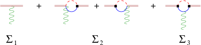
Figure 2: Diagrams contributing to the self-energy of the $\chi$ field at order $v$. Solid, dashed and double lines denote $\Psi,\Phi$ and $\chi$, respectively, and the wiggly line stands for the external field. The shaded squares denote the full three-particle vertex $\gamma(p)$.

The (complex) shift of the pole position to this order is given by

$$\delta P_{*}^{0}=-\frac{v(\Sigma_{1}(P_{*}^{0})+\Sigma_{2}(P_{*}^{0})+\Sigma_{3}(P_{*}^{0}))}{2m_{\chi}+\Sigma_{0}^{\prime}(P_{*}^{0})}+O(v^{2})\,,$$ (20)

where $\Sigma_{0}^{\prime}(P^{0})\doteq\frac{d}{dP^{0}}\,\Sigma_{0}(P^{0})$. Further, using Eq. (8), for the wave function renormalization factor of the $\chi$ particle in the absence of the external field one obtains $Z_{\chi}^{-1}=2m_{\chi}+\Sigma_{0}^{\prime}(P_{*}^{0})$. Consequently, the resonance pole shift (20) in the infinite volume is given by the on-mass-shell vertex function of $\chi$, evaluated at zero momentum transfer

$$\delta P_{*}^{0}=-v\Gamma(0,0)\,,\quad\quad\Gamma(0,0)=Z_{\chi}\,\left(\Sigma_{1}(P_{*}^{0})+\Sigma_{2}(P_{*}^{0})+\Sigma_{3}(P_{*}^{0})\right)\,.$$ (21)

The quantity $\Gamma(0,0)$ is the analog of the magnetic moment of a resonance in our toy model.

Next, we consider the same system in a finite volume. The energy spectrum at $O(v)$ is obtained by solving the equation

$$2m_{\chi}(m_{\chi}-P^{0})-\Sigma_{0}^{L}-v(\Sigma_{1}^{L}+\Sigma_{2}^{L}+\Sigma_{3}^{L})=0\,,$$ (22)

where $\Sigma_{0,1,2,3}^{L}$ are defined by the same expressions as in the infinite volume, where the integration over the loop momentum $k$ is replaced by a discrete sum, see, e.g., Eq. (2).

Suppose that $P^{0}_{m},~{}m\in\mathbb{N}$, is the spectrum at $v=0$. Turning on the external field leads to a shift $P^{0}_{m}\to P^{0}_{m}+\delta P^{0}_{m}$, where $\delta P^{0}_{m}=O(v)$. From Eq. (22) one obtains a relation, which is very similar to Eq. (20) but contains only real variables

$$\delta P_{m}^{0}=-\frac{v(\Sigma_{1}^{L}(P_{m}^{0})+\Sigma_{2}^{L}(P_{m}^{0})+\Sigma_{3}^{L}(P_{m}^{0}))}{2m_{\chi}+(\Sigma_{0}^{L}(P_{m}^{0}))^{\prime}}+O(v^{2})\,,$$ (23)

where

$$\Sigma_{0}^{L}(P^{0}) = \gamma^{2}(p)J^{L}(p)\,,\quad\Sigma_{1}^{L}(P^{0})=\lambda_{1}\,,\quad\Sigma_{2}^{L}(P^{0})=2\lambda_{2}\gamma(p)J^{L}(p)\,,$$

$$\Sigma_{3}^{L}(P^{0}) = \frac{\gamma^{2}(p)}{2w_{\Psi}(p)}\,\frac{d}{dP^{0}}\,J^{L}(p)\biggr{|}_{L=\text{const}}\,,$$ (24)

with $J^{L}(p)$ given by Eq. (14).

One may easily perform the limit $L\to\infty$ in Eq. (23), using $\gamma^{2}(p_{m})J^{L}(p_{m})=2m_{\chi}(m_{\chi}-P^{0}_{m})$ (where $p_{m}$ is defined through $P_{m}^{0}=w_{\Psi}(p_{m})+w_{\Phi}(p_{m})$) and the fact that, for a fixed index $m$, $P_{m}^{0}\to m_{\Psi}+m_{\Phi}$ and $p_{m}\to 0$, as $L\to\infty$. The result is given by

$$\lim_{L\to\infty}\delta P_{m}^{0}=-\frac{v}{2w_{\Psi}(p_{m})}+O(v^{2})\,.$$ (25)

The physical interpretation of the above result is very transparent. Indeed, Eq. (25) exactly reproduces the result obtained in the impulse approximation. This means that a level with any fixed index $m$ disintegrates in the limit $L\to\infty$, and the magnetic moment of a system is given by a sum of the magnetic moments of the constituents $\Psi$ and $\Phi$. In this connection, note that only $\Sigma_{3}$ contributes to Eq. (25) in the limit $L\to\infty$ (e.g., the r.h.s. of this equation does not depend on the couplings $\lambda_{1,2}$). This result, however, clearly does not coincide with the known answer for the magnetic moment in the infinite-volume limit, given by Eq. (20).

On the other hand, let us try extract the pole position on the second Riemann sheet, following exactly the same path as in case with no external field. Namely, measuring the volume-dependent energy spectrum on the lattice $p=p_{m}^{v}(L)$ and inverting this relation $L=L_{m}^{v}(p)$, one may parameterize the quantity

$$p\,\cot\biggl{(}\frac{pL_{m}^{v}(p)}{2}\biggr{)}=\frac{4P^{0}p^{2}}{\gamma^{2}(p)}\,\biggl{(}-2m_{\chi}(m_{\chi}-P^{0})+v(\Sigma_{1}^{L}+\Sigma_{2}^{L}+\Sigma_{3}^{L})\biggr{)}$$ (26)

as a certain known function of a real variable $p$ (see next section for the details). As the next step, one uses this parameterization to continue the expression (26) into the complex plane and finds the shift of the pole position. The result is given by

$$\delta P_{*}^{0}=-\frac{v(\Sigma_{1}^{L}(P_{*}^{0})+\Sigma_{2}^{L}(P_{*}^{0})+\Sigma_{3}^{L}(P_{*}^{0}))}{2m_{\chi}+\Sigma_{0}^{\prime}(P_{*}^{0})}+O(v^{2})\,.$$ (27)

Note that the self-energy operator calculated in the infinite volume, appears in the denominator. Comparing Eqs. (20) and (27), we see that, in order to prove the equivalence of these two expressions at large volumes, one has to investigate – in a finite volume – the analytic continuation of the diagrams shown in Fig. 2 into the complex plane.

4 Analytic continuation

In this section we shall study the analytic continuation of the quantity, which for real values of $p$ is given by Eq. (26). The self-energy in the presence of the external field consists of three contributions $\Sigma_{1,2,3}^{L}$. The analytic continuation of the first contribution is trivial because it is a constant $\Sigma_{1}^{L}(P^{0})=\lambda_{1}$.

The second contribution can be rewritten as

$$\Sigma_{2}^{L}(P^{0})=2\lambda_{2}\gamma(p)J^{L}(p)=\frac{4\lambda_{2}m_{\chi}(m_{\chi}-P^{0})}{\gamma(p)}\,.$$ (28)

It is immediately seen that on the trajectory $L=L_{m}(p)$ the quantity $\Sigma_{2}(P^{0})$ does not depend on the index $m$ (up to exponentially suppressed terms) and is a low-energy polynomial in the variable $p^{2}$: $\Sigma_{2}^{L}(P^{0})=B_{0}+B_{1}p^{2}+\ldots$. The analytic continuation into the complex plane is achieved by substituting $p^{2}\to p_{*}^{2}$. Using Eq. (11), it can be easily shown that on the second Riemann sheet

$$\lim_{p\to p_{*}}\Sigma_{2}^{L}(P^{0})=\frac{-i\lambda_{2}\gamma(p_{*})}{2P^{0}_{*}p_{*}}=2\lambda_{2}\gamma(p_{*})J(p_{*})=\Sigma_{2}(P_{*}^{0})\,,$$ (29)

i.e., the mass-shell limit $p\to p_{*}$ implies the infinite-volume limit $\Sigma_{2}^{L}(P^{0})\to\Sigma_{2}(P_{*}^{0})$.

The situation is more complicated for the last contribution

$$\Sigma_{3}^{L}(P^{0})=\frac{\gamma^{2}(p)w_{\Phi}(p)}{8p^{3}(P^{0})^{2}}\,\biggl{(}\biggl{(}1+\frac{p^{2}}{w_{\psi}(p)w_{\phi}(p)}\biggr{)}\cot\,\pi q_{m}+\pi q_{m}\,(1+\cot^{2}\pi q_{m})\biggr{)}\,,$$ (30)

where $q_{m}=pL_{m}(p)/(2\pi)$. The quantity $\cot\,\pi q_{m}=-p(A_{1}+A_{2}p^{2}+\ldots)$ is proportional to a low-energy polynomial and can be straightforwardly continued in the complex plane. It does not depend on the index $m$. The difficulty comes from the last term which contains the function

$$q_{m}(p)=-\frac{1}{\pi}(\delta(p)-\pi m)=m-\frac{1}{2}+\frac{1}{\pi}\,\text{arccot}(\cot\,\delta(p))\,.$$ (31)

As we see, this expression depends on the index $m$.

The inclusion of $\Sigma_{3}^{L}(P^{0})$ modifies the effective-range expansion in a given constant external field. Namely the expansion of the cotangent of the phase shift now starts at $p^{-2}$, depends on the level index $m$ and contains both odd and even powers in $p$. Note, however, that the dangerous terms are multiplied by the factor $(1+\cot^{2}\pi q_{m})$ which vanishes at the pole after analytic continuation. Consequently, the dependence on the index $m$ in the expression of the pole shift indeed disappears. Note that, in the analytic continuation only the last term in Eq. (31) is potentially problematic, because the arctangent diverges at the pole. However, the factor $(1+\cot^{2}\pi q_{m})$ plays the decisive role. It can be checked that the function $f(z)=(1+z^{2})\,\text{arccot}\,z$, albeit non-analytic at $z=\pm i$, expanded in a Taylor series of $z$, converges to 0 at $z\to\pm i$ (here, $z$ denotes $\cot\,\delta(p)$).

Finally, the procedure of the analytic continuation in the presence of the external field can be formulated as follows. One measures the spectrum $p=p_{m}^{v}(L)$ in the resonance region where $\cot\,\delta(p)$ is small and inverts this relation $L=L_{m}^{v}(p)$. The function $\cot(\frac{1}{2}\,pL_{m}^{v}(p))$ in this region is fitted by the series

$$\cot\biggl{(}\frac{1}{2}\,pL_{m}^{v}(p)\biggr{)}=\frac{D_{-2}}{p^{2}}+\frac{D_{-1}}{p}+D_{0}+D_{1}p+D_{2}p^{2}+\cdots\,,$$ (32)

where the coefficients with even powers of $p$ may depend on the level index $m$ (we recall that the series contains only odd powers of $p$ in the absence of the external field, see Eq. (17)). Finally, after determining the coefficients $D_{i}$ from the fit, we continue the result analytically by substituting $p\to p_{*}$ in this series.

5 Matrix elements at zero momentum transfer

An alternative technique for evaluating the “magnetic moment” in our toy model is to calculate the following Euclidean three-point function on the lattice

$$G(t^{\prime},t)=\langle 0|\Delta(t^{\prime})J(0)\Delta^{\dagger}(t)|0\rangle\,.$$ (33)

Here, $\Delta$ denotes a composite field operator made up from the elementary fields $\Psi$ and $\Phi$, which has the quantum numbers of the $\chi$-particle. Zero total momentum has been projected out by summing up over all spatial locations. Further, $J(0)$ stands for the “current operator” defined through the Lagrangian written down in terms of the elementary fields $\Psi,\Phi$ as ${\cal L}^{v}(0)={\cal L}(0)+vJ(0)+O(v^{2})$. An explicit form of the operators $\Delta,J$ will be inessential in the following. If Euclidean times $t^{\prime},t$ become asymptotically large $t^{\prime}\to+\infty$ and $t\to-\infty$, the three-point function $G(t^{\prime},t)$ goes into

$$G(t^{\prime},t)\rightarrow\langle 0|\Delta(0)|G\rangle\text{e}^{-E_{G}(L)|t^{\prime}|}\langle G|J(0)|G\rangle\text{e}^{-E_{G}(L)|t|}\langle G|\Delta^{\dagger}(0)|0\rangle\,,$$ (34)

where $|G\rangle$ denotes the ground state with the energy $E_{G}(L)$ (we explicitly indicate the dependence on the volume $L$).

On the other hand, the two-point function of the field $\Delta$ at asymptotically large Euclidean times behaves as

$$D(t^{\prime},t)=\langle 0|\Delta(t^{\prime})\Delta^{\dagger}(t)|0\rangle\to\langle 0|\Delta(0)|G\rangle\text{e}^{-E_{G}(L)|t^{\prime}|-E_{G}(L)|t|}\langle G|\Delta^{\dagger}(0)|0\rangle\,.$$ (35)

Extracting the normalization factor $\langle 0|\Delta(0)|G\rangle\langle G|\Delta^{\dagger}(0)|0\rangle$ from Eq. (35) and using this result in Eq. (34), one finally determines the matrix element of the current in the ground state $\langle G|J(0)|G\rangle$. In principle, it is possible to extract the matrix elements between the excited states as well.

The problem consists in the following. As was already mentioned, a resonance does not correspond to any fixed energy level. Then, it is not clear, what is the relation of the matrix element $\langle G|J(0)|G\rangle$ (or, alternatively, of the matrix element between the excited states) to the quantity in the r.h.s. of Eq.(20). After all, this quantity is complex whereas all above matrix elements, extracted from the Euclidean propagators, are real.

In the solution of the above problem, we follow the same path as in the determination of the pole shift in the external field. The three-point function (33) in a finite volume, calculated by using effective field theory, is determined by the diagrams shown in Fig. 2 and the volume dependence of the two-point function is determined by the bubble diagram shown in Fig. 1. Consequently, measuring the current matrix element(s) at different volumes and translating the volume dependence into momentum dependence by invoking the relation $L=L_{m}(p)$, as discussed in section 4, one may parameterize these matrix element(s) in terms of known functions of $p$ on the real axis. The final step consists in the substitution $p\to p_{*}$ in these expressions, which yield the complex quantity coinciding with the r.h.s. of Eq. (20).

Finally, we note that by using the same method, it is possible to study the form factors at non-zero momentum transfer. We, however, prefer to address this question separately.

6 Conclusions

Placing a stable particle in a constant external field leads to a shift of its mass. To first order in the external field, the shift is given by the form factor of the particle at zero momentum transfer. The calculations on the lattice can be carried out straightforwardly.

In case of a resonance, the interpretation of the lattice results is difficult, because a resonance is not described by an isolated energy level in the energy spectrum. In particular, the form factor of a resonance even at zero momentum transfer is a complex quantity, whereas all energy shifts are real.

Using non-relativistic effective field theory technique, we have described the procedure of the extraction of the resonance form factor (at zero momentum transfer) from the Euclidean lattice data in 1+1 dimensions. This procedure can be regarded as a generalization of Lüscher’s approach to the form factors of the resonances. In brief, the method consists of the following steps: In the absence of the external field, one assumes that the effective range expansion is convergent in the resonance region. Using this fact, one may analytically continue the cotangent of the scattering phase into the complex plane and determine the location of a resonance pole on the second Riemann sheet. Further, it is shown that the form of the effective range expansion gets modified in the presence of the external field. Using the modified expansion, one again performs the analytic continuation into the complex plane and determines the shift of the pole position in the external field.

The main result of the article consists in the following. It is demonstrated that the pole shift in a finite volume up to exponentially vanishing terms, is determined by the resonance form factor calculated in the infinite volume. The key observation, which leads to this result, is that approaching the resonance pole position $p\to p_{*}$ in the complex plane simultaneously implies the infinite-volume limit $\lim_{p\to p_{*}}\text{Im}\,q=-\infty$.

The resonance form factor can be evaluated by using an alternative technique as well. Namely, it is possible to directly calculate the corresponding three-point function on the lattice and study its asymptotic behavior at large Euclidean times. It has been shown in the present paper that by applying the same method it is possible to construct the resonance form factor at zero momentum transfer from of the current matrix elements between eigenstates of a Hamiltonian in a finite volume that are determined by measuring the three-point function.

Finally, it should be stressed that in the case of 3+1 dimensions, so-called finite fixed points may exist. These fixed points obey the condition $\lim_{p\to p_{*}}|q|<\infty$ and thus invalidate the proof, given in section 4. It remains to be clarified, whether the proof can be adapted to this case as well. We plan to address this issue in future publications.

Acknowledgments. We thank J. Gasser, J. Gegelia, M. Göckeler, H.-W. Hammer, T. Hemmert, F. Niedermaier, V. Pascalutsa, A. Schäfer, G. Schierholz, C. Urbach and M. Vanderhaeghen for interesting discussions.

Appendix A The loop function

To calculate the function $J(p)$ displayed in Eq. (4), we first perform the integration over the variable $k^{0}$ using Cauchy’s theorem. The result in the center-of-mass frame is given by

$$J(p)=\int\frac{d^{d}k}{(2\pi)^{d}}\frac{1}{2w_{\Psi}(k)2w_{\Phi}(k)}\,\frac{1}{\left(w_{\Psi}(k)+w_{\Phi}(k)-P^{0}\right)}\,,\quad d=D-1\,.$$ (A.1)

The integrand in the above equation can be identically rewritten in the following form:

$$\frac{1}{2w_{\Psi}(k)2w_{\Phi}(k)}\,\frac{1}{\left(w_{\Psi}(k)+w_{\Phi}(k)-P^{0}\right)} = \frac{1}{2P^{0}}\,\frac{1}{k^{2}-p^{2}}$$ (A.2)

$$+ \frac{1}{2w_{\Psi}(k)2w_{\Phi}(k)}\,\frac{1}{\left(w_{\Psi}(k)+w_{\Phi}(k)+P^{0}\right)}$$

$$+ \frac{1}{2w_{\Psi}(k)2w_{\Phi}(k)}\,\frac{1}{\left(w_{\Psi}(k)-w_{\Phi}(k)-P^{0}\right)}$$

$$+ \frac{1}{2w_{\Psi}(k)2w_{\Phi}(k)}\,\frac{1}{\left(w_{\Phi}(k)-w_{\Psi}(k)-P^{0}\right)}\,.$$

The calculation of the integral given by Eq. (A.1) proceeds as follows [18]. One first expands the integrand in powers of momenta, integrates the result using the dimensional regularization and sums up the resulting series. Doing this, the last three terms on the r.h.s. of Eq. (A.2) vanish after integration, because the integrands turn into polynomials in the momenta. The non-vanishing result, given in Eq. (4), is obtained by the integration of the first term.

The calculation of the loop function in a finite volume follows a similar path. We again perform the integration over the variable $k^{0}$ and use the identity Eq. (A.2). The sum over the momenta $k$ in the last three terms (non-singular) exponentially vanishes for large $L$ (see, e.g., Ref. [20]) and can therefore be omitted. Hence, up to these terms, the quantity $J^{L}(p)$ from Eq. (2) is given by

$$J^{L}(p)=\frac{1}{2P^{0}L}\,\sum_{k}\frac{1}{k^{2}-p^{2}}=\frac{1}{2P^{0}L}\,\int_{-\infty}^{\infty}\frac{dl}{l^{2}-p^{2}}\,\sum_{n=-\infty}^{\infty}\delta\biggl{(}l-\frac{2\pi}{L}\,n\biggr{)}\,.$$ (A.3)

We calculate this expression first below threshold, $p=i\kappa$. Using the Poisson identity

$$\sum_{n=-\infty}^{\infty}\delta(x-n)=\sum_{n=-\infty}^{\infty}\text{e}^{2\pi ixn}$$ (A.4)

and integrating over the variable $l$ with the help of Cauchy’s theorem, we get

$$J^{L}(p)=\frac{1}{4P^{0}\kappa}\,\biggl{(}2\sum_{n=0}^{\infty}\text{e}^{-n\kappa L}-1\biggr{)}\,.$$ (A.5)

Summing up the geometric series in Eq. (A.5) and continuing analytically to the real values of $p$ by substituting $\kappa=-ip$, we finally obtain the expression given in Eq. (14). This expression is nothing but Lüscher’s zeta-function in 1+1 dimensions.

References

- [1] C. W. Bernard, T. Draper, K. Olynyk and M. Rushton, Phys. Rev. Lett. 49 (1982) 1076.
- [2] F. X. Lee, R. Kelly, L. Zhou and W. Wilcox, Phys. Lett. B 627 (2005) 71 [arXiv:hep-lat/0509067].
-
[3]
F. X. Lee, S. Moerschbacher and W. Wilcox,
Phys. Rev. D 78 (2008) 094502
[arXiv:0807.4150 [hep-lat]]. - [4] C. Aubin, K. Orginos, V. Pascalutsa and M. Vanderhaeghen, [arXiv:0811.2440 [hep-lat]].
- [5] J. C. Christensen, W. Wilcox, F. X. Lee and L. m. Zhou, Phys. Rev. D 72 (2005) 034503 [arXiv:hep-lat/0408024].
- [6] F. X. Lee, L. Zhou, W. Wilcox and J. C. Christensen, Phys. Rev. D 73 (2006) 034503 [arXiv:hep-lat/0509065].
- [7] W. Detmold, B. C. Tiburzi and A. Walker-Loud, Phys. Rev. D 79 (2009) 094505 [arXiv:0904.1586 [hep-lat]].
- [8] W. Detmold, B. C. Tiburzi and A. Walker-Loud, arXiv:1001.1131 [hep-lat].
- [9] C. Alexandrou, T. Korzec, T. Leontiou, J. W. Negele and A. Tsapalis, PoS LAT2007 (2007) 149 [arXiv:0710.2744 [hep-lat]].
- [10] C. Alexandrou et al., Phys. Rev. D 79 (2009) 014507 [arXiv:0810.3976 [hep-lat]].
- [11] M. Lüscher, DESY-88-156 Lectures given at Summer School ’Fields, Strings and Critical Phenomena’, Les Houches, France, Jun 28 - Aug 5, 1988; U.-J. Wiese, Nucl. Phys. Proc. Suppl. 9 (1989) 609; M. Lüscher, Nucl. Phys. B 354 (1991) 531; M. Lüscher, Nucl. Phys. B 364 (1991) 237.
- [12] S. R. Beane, P. F. Bedaque, A. Parreno and M. J. Savage, Nucl. Phys. A 747 (2005) 55 [arXiv:nucl-th/0311027].
-
[13]
V. Bernard, M. Lage, U.-G. Meißner and A. Rusetsky,
JHEP 0808 (2008) 024
[arXiv:0806.4495 [hep-lat]]. - [14] M. Lage, U.-G. Meißner and A. Rusetsky, Phys. Lett. B 681 (2009) 439 [arXiv:0905.0069 [hep-lat]].
- [15] J. Hu, F. J. Jiang and B. C. Tiburzi, Phys. Lett. B 653 (2007) 350 [arXiv:0706.3408 [hep-lat]].
- [16] B. C. Tiburzi, Phys. Rev. D 77 (2008) 014510 [arXiv:0710.3577 [hep-lat]].
- [17] B. C. Tiburzi, Phys. Lett. B 674 (2009) 336 [arXiv:0809.1886 [hep-lat]].
- [18] G. Colangelo, J. Gasser, B. Kubis and A. Rusetsky, Phys. Lett. B 638 (2006) 187 [arXiv:hep-ph/0604084].
- [19] J. Gegelia and S. Scherer, arXiv:0910.4280 [hep-ph].
- [20] C. H. Kim, C. T. Sachrajda and S. R. Sharpe, Nucl. Phys. B 727 (2005) 218 [arXiv:hep-lat/0507006].