The Radio Properties of Type 2 Quasars

Abstract

This paper presents the first high-resolution and high-sensitivity study of the radio properties of optically selected type 2 quasars. We used the Very Large Array at 8.4 GHz to observe 59 sources drawn from the Sloan Digital Sky Survey sample of Zakamska et al. (2003). The detection rate of our survey is 59% (35/59), comparable to the detection rate in FIRST at 1.4 GHz. Ongoing star formation, although present, contributes negligible radio emission at the current sensitivity limit. Comparing the radio powers with the [O III] $\lambda$5007 luminosities, we find that roughly 15%$\pm$5% of the sample can be considered radio-loud. Intriguingly, the vast majority of the detected sources in our sample fall in a region intermediate between those traditionally occupied by radio-loud and radio-quiet quasars. Moreover, most of these “radio-intermediate” sources tend to have flat or inverted radio spectra, which we speculate may be caused by free-free absorption by ionized gas in the narrow-line region. The incidence of flat-spectrum sources in type 2 quasars appears to be much higher than in type 1 quasars, in apparent violation of the simple orientation-based unified model for active galaxies.

1 Introduction

The collective properties of active galactic nuclei (AGNs) can be understood within the framework of unification models in which the observed properties of active galaxies are governed primarily by orientation, intrinsic luminosity, and Eddington ratio (Antonucci 1993; Urry & Padovani 1995; Ho 2008). Many of the apparent differences between type 1 (broad-line) and type 2 (narrow-line) AGNs can be attributed to our line-of-sight having different orientations with respect to the disk. In conventional unified models of active galaxies, the accretion disk and broad-line region are surrounded by a dusty molecular torus. In type 2 AGNs, where the view being edge-on, the torus blocks a direct view of the continuum and broad-line region, which can only be detected through light scattered into the line-of-sight by material lying directly above the torus opening; by contrast, in type 1 AGNs, the view being pole-in, the continuum and broad-line region can be viewed directly. The basic predictions of this geometric unification scheme have enjoyed much success in the context of Seyfert galaxies (e.g., Antonucci 1993; Lal et al. 2004). A natural question is whether this simple picture extends to AGNs of higher luminosity: are there type 2 quasars?

As an alternative to the classical orientation-based unification scheme, wherein the obscuration arises solely from a nuclear-scale dusty torus, the obscuration in type 2 quasars may largely come instead from the large-scale distribution of dust in the host, which is itself tied to the evolutionary state of the galaxy. For example, the hierarchical buildup of galaxies through major mergers of gas-rich progenitors naturally produces remnants with copious stockpiles of centrally concentrated gas and dust, which not only fuels a major starburst but also often accretion onto a highly obscured AGN (e.g., Sanders & Mirabel 1996; Genzel et al. 1998). If sufficiently powerful, the buried AGN in these ultraluminous infrared systems would qualify as type 2 quasars. Over time, as the gas and dust get depleted through consumption and expulsion from energy feedback, the AGN transitions from an obscured to an unobscured source (e.g., Sanders et al. 1988; Hopkins et al. 2006). In this picture, type 2 quasars are the evolutionary precursors of, and intrinsically different from, type 1 quasars.

A large body of work over the last several years has established beyond doubt that type 2 quasars truly do exist. Individual case studies (e.g., Dawson et al. 2001; Norman et al. 2002; Stern et al. 2002; Derry et al. 2003; Jarvis et al. 2005) have given way to large systematic searches for obscured quasars from hard X-ray (e.g., Ueda et al. 2003; Sazonov et al. 2007), infrared (e.g., Lacy et al. 2004; Polletta et al. 2008), and optical (Zakamska et al. 2003; Dong et al. 2005; Reyes et al. 2008) surveys. The Sloan Digital Sky Survey (SDSS; York et al. 2000) makes it possible to find substantial numbers of optically selected type 2 quasar candidates. The first results from Zakamska et al. (2003) produced a large sample of 291 objects at redshift 0.3 $<$ $z$ $<$ 0.83; the sample includes Seyfert 2 galaxies as well as objects luminous enough to qualify as type 2 quasar candidates. The latest update from Reyes et al. (2008) has increased the list of candidates to nearly 900 sources. The overall concensus seems to be that type 2 quasars constitute an important component of the general AGN population. In a related development, radio and infrared selection have revealed increasingly large numbers of red quasars (e.g., Webster et al. 1995; Gregg et al. 2002; Richards et al. 2003; White et al. 2003), whose nonstandard colors in most cases can be attributed to increased dust reddening (e.g., Glikman et al. 2007), perhaps linked to galaxy mergers (Urrutia et al. 2008). The prevalence of high-luminosity obscured or dusty AGNs has important implications for a wide range of broader astrophysical issues, ranging from testing the classical unification model of AGNs to understanding the origin of the cosmic X-ray background (e.g., Madau et al. 1994; Comastri et al. 1995), the accretion history of supermassive black holes (e.g., Martínez-Sansigre & Taylor 2009), and the coevolution of black holes and galaxies (e.g., Greene et al. 2009).

To better understand the physical characteristics of type 2 quasars and their relation to other classes of AGNs, it is essential to define the multiwavelength properties of these objects. To date, follow-up studies have concentrated mostly on the initial SDSS sample of Zakamska et al. (2003), investigating their optical spectropolarimetric (Zakamska et al. 2005), emission-line (Villar-Martín et al. 2008), X-ray (Vignali et al. 2004, 2006; Ptak et al. 2006), infrared (Zakamska et al. 2008), and host galaxy (Zakamska et al. 2006; Greene et al. 2009; Liu et al. 2009) properties. Zakamska et al. (2004) assembled sky-survey data at radio, infrared, optical, and soft X-ray wavelengths, concluding that the broadband properties of the sample support the thesis that the narrow-line SDSS sources are obscured (type 2) quasars.

This contribution presents new 8.4 GHz Very Large Array (VLA) observations of a subset of the SDSS type 2 quasars. Notwithstanding the work of Zakamska et al. (2004), relatively little is actually known about the detailed radio properties of this new population of AGNs. Using radio data primarily from the 1.4 GHz FIRST survey (Becker et al. 1995), which has a root-mean-square (rms) sensitivity of $\sim$0.15 mJy, Zakamska et al. (2004) reported that less than half of the sample sources have radio counterparts. At the resolution of FIRST ($\sim$5^′′), the vast majority of the radio detections have a simple compact morphology. Very limited information was given for the radio spectral shape, being limited to low-resolution data for the few brightest sources with extended morphologies.

Our new 8.4 GHz observations represent a nearly ten-fold increase in sensitivity (rms $\approx 0.02$ mJy) and an improvement in resolution by more than a factor of 6 (beam $\sim$0$\farcs$8). These improvements allow us to better delineate the basic radio properties of these sources, including their distribution of radio powers, source structure, and, in combination with the extant 1.4 GHz observations, spectral indices.

Distance-dependent quantities are calculated assuming $H_{0}$ = 70 km s^-1 Mpc^-1, $\Omega_{m}$ = 0.3, and $\Omega_{\Lambda}$ = 0.7. Throughout the paper we define the spectral index $\alpha$ in the sense that $S_{\nu}\propto\nu^{\alpha}$, where $S_{\nu}$ is the flux density and $\nu$ is the frequency.

2 Data

2.1 Sample

Our targets are drawn from the type 2 quasar sample of Zakamska et al. (2003). This is the first comprehensive sample of such sources, for which we understand the optical properties in great detail. The SDSS sources have a wide range of AGN power, ranging from luminosities in the regime of Seyfert galaxies to quasars. Most of the sources qualify as quasars according to the [O III] $\lambda$5007 luminosity criterion of Zakamska et al. (2003). Although the [O III] $\lambda$5007 emission might be mildly anisotropic (Hes et al. 1996; but see Kuraszkiewicz et al. 2000), it is widely used as a measure of intrinsic AGN power for both type 1 and type 2 sources (e.g., Lal et al. 2004; Heckman et al. 2005).

Given the time allotted to our VLA program, we have decided to pick a subset of the SDSS sample in a restricted window in [O III] luminosity in order to explore its full range of radio properties. Our final choice focuses on the 59 sources, $\sim$20% of the 291 sources in Zakamska et al. (2003), in the luminosity range $L_{\rm[O~{}\sc III]}=10^{41.8}-10^{42.1}$ erg s^-1, which coincides with the peak of the [O III] luminosity distribution and satisfies the formal luminosity definition of type 2 quasars (Figure 1). The sources are distributed in the redshift range 0.3 $\mathrel{\hbox{\hbox to0.0pt{\hbox{\lower 4.0pt\hbox{$\sim$}}\hss}\hbox{$<$}}}$ $z$ $\mathrel{\hbox{\hbox to0.0pt{\hbox{\lower 4.0pt\hbox{$\sim$}}\hss}\hbox{$<$}}}$ 0.8, with an average value of $z\approx 0.45$.

2.2 Observations

We were granted 24 hours of observing time for our program (program code AV288). The observations were carried out in snapshot mode in a single observing run on 2006 July 24–25, with the VLA in B configuration, with two 50 MHz intermediate-frequency (IF) channels at a mean frequency of 8.4351 GHz (see Table 1). This provided a typical resolution of $\sim$ $0\hbox{$.\!\!^{\prime\prime}$}8$. The weather conditions were excellent during the observing session. Since we are mainly concerned with the emission from the source, which is placed at the phase-tracking center, bandwidth smearing (Bridle & Schwab 1999) is not a problem at 8.4 GHz despite the somewhat large bandwidth. The excellent sensitivity of the 8.4 GHz receivers of the VLA routinely permits high signal-to-noise ratio maps to be made in relatively short integration times (snapshot mode). Each scan yielding a total exposure time of $\sim$ 15$-$18 minutes for target source was interleaved with 2–3 minute scans on a suitable secondary VLA flux calibrator. Due to the wide range of right ascensions in the sample, some of the sources could only be observed when they were close to rising or setting, and consequently the synthesized beams were highly distorted. More than half the phase calibrators used have position accuracies of 0$\farcs$01 or better, and the rest of the calibrators have position accuracies of $\sim$0$\farcs$1. Multiple observations of 3C 147 and 3C 286 were used to tie the absolute fluxes to the VLA scale.

2.3 Data Reduction

The data were processed with the Astronomical Image Processing System (AIPS; version 31DEC03) package. We used R. Perley’s revised coefficients for flux density calibration (Baars et al. 1977) as described in the AIPS Cookbook. Errors in the quoted flux densities are dominated by the uncertainty in setting the absolute flux density scale, with the conservative estimate being 5%. The data were Fourier transformed using AIPS task IMAGR with uniform weighting in order to maximise resolution, and after CLEAN deconvolution, the maps were restored. Since we do not know the morphological details of the sources, we mapped the primary beam area (5$\farcm$3) with a cell size of 0$\farcs$1. The mapped region is larger than the typical size of the extended sources mentioned in Zakamska et al. (2003). The number of CLEAN iterations was set so that the minimum clean component reached 0.04 mJy beam^-1, $\sim$2 times the theoretical thermal noise limit of the maps. Stronger sources (such as SDSS J0329$+$0052 or SDSS J2354$-$0056), whose maps were not limited by the system noise, were subjected to several cycles of phase-only self-calibration until the sensitivity approached thermal noise levels. A model based on the CLEAN components was used to start the self-calibration process. We also performed phase-only self-calibration for one or two iterations for the weakly detected sources, but the improvement was minimal. At each round of self-calibration, the image and the visibilities were compared to check for the improvement in the source model. The two IFs were calibrated and mapped separately with the intention of concatenating the two sets of data for each source. The IF1 images suffered consistently from higher noise levels, however, and it was therefore decided to use the maps from IF2 (8.4601 GHz) only. The self-calibration typically moved source positions by less than 0$\farcs$01, indicating that atmospheric phase irregularities had a relatively small effect on source positions. Therefore, in most cases, the measured positions are accurate to 0$\farcs$1 or better. The theoretical rms noise of our snapshot images is expected to be 0.02 mJy beam^-1, a level attained in almost all of the maps.

We constructed images at two different resolutions by applying appropriate tapering functions to the visibilities. Two sets of total intensity (Stokes $I$) maps were made, one at full resolution (Figure 2) and another with a Gaussian tapering function falling to 20% of full resolution (Figure 3), which (nearly) corresponds to a synthesized beam matching the FIRST survey maps. The latter tapered maps were used to assess the possible presence of extended emission, to evaluate the spectral indices, and to examine structural counterparts between the 8.4 GHz and 1.4 GHz maps.

3 Results

3.1 Maps and Source Parameters

Our results are shown in Figure 2 for all 59 sources, including 24 nondetections. Sources are arranged in the order of increasing RA. The restoring beam is depicted as an ellipse on the lower left-hand corner of each map. The contour levels of the maps are rms $\times$ ($-$3, 3, 6, 12, 24, 48, …), where the rms values for the maps are given in Table 2 (Column 5). The optical position of the galaxy is marked with a cross, the semi-major length of which corresponds to the 3 $\sigma$ uncertainty of $\sim$0$\farcs$3 for the SDSS astrometry (Pier et al. 2003).

The dynamic range (peak/noise) of the maps lies between $\sim 3$ and 465. We have adopted a consistent method in extracting source parameters. The rms noise of each map is determined from a source-free, rectangular region. The galaxy is considered detected if a source with a peak flux density at least 5 times the rms is found within the error box of the optical position. For undetected sources, the upper limit is set to 5 times the rms. Whenever possible we determined the source parameters — integrated flux density and deconvolved (half maximum) sizes (major and minor axis) — by fitting a two-dimensional Gaussian model using the AIPS task JMFIT. This procedure works well for sources with relatively simple, symmetric structure, such as most galaxy cores and pointlike features. For components with more complex morphologies, or for weak, marginal detections, we simply integrated the signal within interactively defined boundaries, using the AIPS task IMEAN for rectangular boxes and TVSTAT for irregularly shaped regions. A source is considered resolved if its deconvolved size is larger than one-half the beam size at full width at half-maximum (FWHM) in at least one of the two dimensions.

Table 2 lists the map and source parameters. The columns are as follows: (1) SDSS galaxy name, which also encodes the optical position of the source; (2) FWHM of the elliptical Gaussian restoring beam; (3) P.A. of the restoring beam; (4) flux density of the source at 8.4 GHz as measured in the default, high-resolution map; (5) rms noise of the map; and (6) comments on the source structure. We have also gathered 1.4 GHz data from FIRST (Columns 7 and 8). The typical detection threshold is 0.75 mJy, and when neither a FIRST nor an NVSS (Condon et al. 1998) detection is available, we use this threshold as the upper limit. Columns (9) and (10) list the corresponding parameters for the tapered maps at 8.4 GHz, matched to the resolution of FIRST. Finally, Column (11) gives the spectral index between 1.4 GHz and 8.4 GHz for the core and detected components; we have not assigned formal error bars to the measurements, but the uncertainty for a typical 1–5 mJy source is 0.04–0.07. The low-resolution maps have restoring beams of size 5$\farcs$4$\times$5$\farcs$4 for sources with declination $\delta$ $>$30^∘ and 6$\farcs$4$\times$5$\farcs$4 for sources with declination $-5$^∘ $<$ $\delta$ $<$ 10^∘ (an exception is SDSS J0257$-$0632, which has a beam of 6$\farcs$8$\times$5$\farcs$4).

A compilation of derived radio parameters, along with optical parameters, is given in Table 3. The columns are as follows: (1) galaxy name; (2) redshift, as determined by SDSS; (3) luminosity distance; (4) total, integrated monochromatic power at 1.4 GHz and (5) 8.4 GHz; and (6) the radio morphology of the sources shown in the maps presented. We adopt the definitions of Ho & Ulvestad (2001) and Ulvestad & Wilson (1984) for the radio morphology classes: “U” (single, unresolved), “S” (single, slightly resolved), “D” (diffuse), “L” (linear structure, or multiply aligned components), and “E” (extended diffuse). Following Ho & Ulvestad (2001), a slightly resolved source is one whose deconvolved size is $\geq$ $\frac{1}{2}$ the synthesized beam width. Radio powers in the source frame that were emitted in our observed frequencies were computed from the flux densities using Ned Wright’s online cosmology calculator. The radio powers $P^{\rm tot}_{1.4}$ and $P^{\rm tot}_{8.4}$ have been $K$-corrected to the restframe of each source, such that $P_{\nu}=4\pi D_{L}^{2}S_{\nu}(1+z)^{-1-\alpha}$, with $D_{L}$ being the luminosity distance, $S_{\nu}$ the observed flux density, and $\alpha$ the spectral index. For the undetected sources, we adopt the median spectral index of the detected sources ($\alpha^{8.4}_{1.4}=+0.094$; see below). The last two columns of the table give the luminosity of the (7) [O II] $\lambda$3727 and (8) [O III] $\lambda$5007 lines, taken from Zakamska et al. (2003). Additional notes on some selected objects are given in the Appendix.

4 Discussion

4.1 Basic Radio Properties

To a depth of rms $\approx$ 20 $\mu$Jy beam^-1, the detection rate of our 8.4 GHz survey is 59% (35/59). Remarkably, this detection rate is essentially identical to that obtained from FIRST at 1.4 GHz, which observed 56 out of the 59 sources in our sample and detected 35 (63%), even though the sensitivity of FIRST is nearly an order of magnitude lower than that of our X-band survey. Moreover, our 8.4 GHz observations did not yield any new detections that were not already contained in FIRST. The detection rate in FIRST for our subsample of type 2 quasars agrees well with the overall detection rate reported for the original SDSS sample from Zakamska et al. (2003) (46%), as well as for the larger, updated sample from Reyes et al. (2008) (61%). Restricting the Reyes et al. sample to the 86 objects that meet the same selection criteria employed in this study ($z>0.3$ and $L_{\rm[O~{}\sc III]}=10^{41.8}-10^{42.1}$ erg s^-1), the detection rate in FIRST becomes 53%, again compatible with ours.

At our arcsecond-scale resolution, the morphology of the radio emission is predominantly that of a compact core, either unresolved or slightly resolved (75% of the detections classified as “U” or “S”). At an average redshift of $z=0.45$, our 0$\farcs$8 beam corresponds to a physical diameter of 4.6 kpc. Higher-resolution observations may begin to resolve this emission into subgalactic-scale structures with physical dimensions below 1 kpc, as often seen in nearby Seyfert galaxies (e.g., Ho & Ulvestad 2001). Six sources ($\sim$10%) have very extended, supergalactic-scale structures (see Figure 3). The maximum linear extents are enormous, five out of the six having diameters approaching 1 Mpc, comparable to the sizes of the largest radio galaxies (e.g., Machalski & Jamrozy 2006). Down to the 3 $\sigma$ contour level of the 1.4 GHz maps, the following are the maximum linear extents: 177 kpc (SDSS J0040$-$0040), 868 kpc (SDSS J0257$-$0632), 709 kpc (SDSS J0902$+$5459), 847 kpc (SDSS J1008$+$4613), 797 kpc (SDSS J1247$+$0152), and 894 kpc (SDSS J2157$+$0037). All but SDSS J1247$+$0152 have steep spectra (average $\alpha^{8.4}_{1.4}=-0.87$), the latter being relatively flatter with $\alpha^{8.4}_{1.4}=-0.41$.

Normal, inactive $L^{*}$ galaxies have a characteristic radio power of $\sim 10^{28}$ erg s^-1 Hz^-1 at 1.4 GHz (Condon 1992; de Vries et al. 2007). Our sample of type 2 quasars is roughly 2–4.5 orders of magnitude more powerful (Figure 4). Accounting for the upper limits using the Kaplan-Meier product-limit estimator (Feigelson & Nelson 1985), the mean radio power is $7.29\times 10^{31}$ erg s^-1 Hz^-1 at 1.4 GHz and $1.99\times 10^{31}$ erg s^-1 Hz^-1 at 8.4 GHz; the corresponding medians are $1.69\times 10^{30}$ and $3.67\times 10^{30}$ erg s^-1 Hz^-1. It is interesting to note that the distribution of radio powers at 8.4 GHz shows an apparent gap between the bulk of the detections and the upper limits: there appears to be an absence of points near $P^{\rm tot}_{8.4}\approx 10^{30}$ erg s^-1 Hz^-1. This could indicate that the detected and undetected sources define two distinctly different populations.

By combining the 1.4 GHz FIRST measurements with our tapered, matched-resolution 8.4 GHz maps, we are able to determine spectral indices for all the detected components. Because the two bands were not observed contemporaneously, we caution that the spectral index for any individual source might be affected by variability. We do not know whether type 2 quasars vary in the radio, but if they are similar to type 1 quasars (Barvainis et al. 1996, 2005), they should. The statistical ensemble properties of the sample, however, should be quite robust to the effects of individual source variability. A surprising aspect of our results is the preponderance of sources with rather flat to highly inverted spectral indices (Figure 5). For the subset of detected sources, $\alpha^{8.4}_{1.4}$ has an average value of $-0.10$, a standard deviation of 0.65, and a median value of $+0.094$. Twenty-three out of the 36 (64%) sources with spectral index measurements have $\alpha^{8.4}_{1.4}>-0.5$, a commonly used definition for a flat spectrum. Curiously, the distribution of spectral indices appears bimodal: there is a peak centered at $\alpha^{8.4}_{1.4}\approx-0.7$, one centered at $\sim+0.6$, and an apparent minimum near $\alpha^{8.4}_{1.4}=0$. Based on a small number of objects with available multifrequency measurements, Zakamska et al. (2004) concluded that type 2 quasars tend to have relatively steep radio spectra, most with $\alpha$ $\mathrel{\hbox{\hbox to0.0pt{\hbox{\lower 4.0pt\hbox{$\sim$}}\hss}\hbox{$<$}}}$ $-0.5$. This result, however, is biased toward the minority of objects that had low-resolution literature data, most being powerful, steep-spectrum sources. In a similar vein, the population of high-redshift ($z\approx 2$) type 2 quasars studied by Martínez-Sansigre et al. (2006) is dominated by relatively powerful, steep-spectrum ($\alpha\approx-1$) sources. By contrast, our study, concentrating on the more typical members of the population, indicates the opposite — the majority of optically selected type 2 quasars have flat radio spectra. Plotting the 1.4 GHz power as a function of spectral index (Figure 6) reveals the interesting trend that the spectral index becomes progressively flatter with decreasing radio power. Rather than a tight correlation, the trend can best be described as an upper envelope: when $\alpha$ is steep, the radio power spans a very wide range (in this sample, up to 3 orders of magnitude), but as $\alpha$ flattens, the range of radio power narrows systematically, until it converges to a $P^{\rm tot}_{1.4}\approx 10^{30}$ erg s^-1 Hz^-1 with a remarkably tiny spread ($\sim$0.2 dex) when $\alpha^{8.4}_{1.4}$ approaches $+0.9$. If we focus on the population with $P^{\rm tot}_{1.4}$ $\mathrel{\hbox{\hbox to0.0pt{\hbox{\lower 4.0pt\hbox{$\sim$}}\hss}\hbox{$<$}}}$ $10^{31}$ erg s^-1 Hz^-1, close to the traditional luminosity-based criterion for radio-quiet AGNs (e.g., Miller et al. 1990; Hooper et al. 1995), essentially all sources are flat-spectrum.

Most of the sources with $\alpha^{8.4}_{1.4}\geq 0$ have a compact radio structure, but, interestingly, not all compact sources have a flat or inverted spectrum. SDSS J0316$-$0059, J0903$+$0211, J0908$+$4347, J1539$+$5142, and J2354$-$0056 all have compact structures but are steep-spectrum; they are also moderately radio-loud (see Section 4.2). These may be analogs of compact steep-spectrum sources (Fanti et al. 1990), although classical compact steep-spectrum sources are 2–3 orders of magnitude more luminous than our objects (O’Dea 1998). Conversely, while extended, linear features are typically steep-spectrum (e.g., SDSS J0257$-$0632, J0902$+$5459, J1008$+$4613), there are some examples of double-lobed structures that have clearly flat or inverted spectra (e.g., SDSS J0741$+$3020, J1014$+$0244). This is unusual, but not without precedence (e.g., Lal & Rao 2007).

Comparable statistics for the spectral indices of radio-quiet type 1 quasars in the GHz range are fragmentary and highly incomplete. Nevertheless, to get a rough comparison, we compiled available measurements for low-redshift radio-quiet quasars, drawn from the studies of Barvainis et al. (1996, 2005), Kukula et al. (1998), and Ulvestad et al. (2005). Similar to our observations, all of these measurements were made with the VLA, and the frequency coverage was from 1.4 GHz to either 5 or 8.4 GHz. For a heterogeneous collection of 73 objects, we find a mean spectral index of $-0.46$ and a median value of $-0.59$; 51% qualify as flat-spectrum ($\alpha>-0.5$). Falcke et al. (1996) conducted a quasi-simultaneous single-dish survey at 2.7 and 10 GHz of all Palomar-Green (Schmidt & Green 1983) quasars with 4.9 GHz flux densities greater than 4 mJy. For the 25 radio-quiet sources (those with $R<10$ as defined by Kellermann et al. 1989) with tabulated spectral indices, we find a mean value of $-0.66$ and a median value of $-0.60$; 28% of these qualify as flat-spectrum. Although a more rigorous control sample of type 1 quasars would clearly be desirable, the above comparison suggests that flat-spectrum sources are much more prevalent in type 2 quasars than in type 1 quasars. Taken at face value, this implies that the two classes are not intrinsically the same, in apparent violation of the simplest notions of the orientation-based unified model.

4.2 The Nature of the Radio-Intermediate, Flat-Spectrum Sources

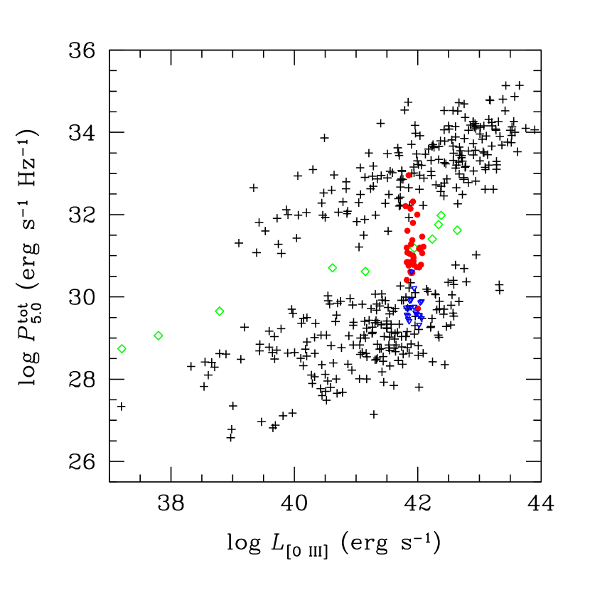
Figure 7: Correlation between radio power and [O III] luminosity. The plus symbols come from the sample of Xu et al. (1999), with the open green diamonds representing their radio-intermediate sources. The data from Xu et al. were taken at 5 GHz and have been corrected to our adopted cosmological parameters and to our units for the monochromatic radio power. Our sample sources are shown as filled red circles, with upper limits marked as open blue triangles. We converted our measurements to 5 GHz using the observed spectral index for each detected source; for the nondetections, we use the median spectral index of the detected sources.

The radio output of type 1 quasars (e.g., Kellermann et al. 1989) and lower luminosity Seyfert 1 nuclei (e.g., Ho & Peng 2001) is conventionally specified by referencing the radio band with respect to the broadband optical continuum. This definition of “radio-loudness” cannot be used for obscured, type 2 sources, but the luminosity of the largely isotropic narrow emission lines can be used instead to substitute for the optical continuum. Figure 7 illustrates the distribution of integrated radio power (at 5 GHz) versus [O III] luminosity for a large, heterogeneous sample of AGNs compiled by Xu et al. (1999). The points clearly delineate two nearly parallel sequences, albeit each with significant scatter, separated by a pronounced gap. Roughly $15\%\pm 5\%$ of our sample lie on the radio-loud branch. Within the somewhat nebulous definition of this nomenclature and the small statistics of our sample, this is consistent with the radio-loud fraction ($9\%\pm 2\%$) quoted by Zakamska et al. (2004) for the parent SDSS sample, which in turn is consistent with the nominal radio-loud fraction of type 1 quasars ($\sim 10\%-20\%$; Kellermann et al. 1989; Hooper et al. 1995; Ivezić et al. 2002). Not surprisingly, all the nondetections are in the radio-quiet branch. Figure 8 gives a magnified view of our sample alone. As already noted above, all but one of the 8.4 GHz upper limits seem to define a population separate from the detected objects; there appears to be a genuine dearth of points near $P^{\rm tot}_{8.4}\approx 10^{30}$ erg s^-1 Hz^-1.

Within the Xu et al. (1999) sample, a small number of objects (3%; marked as green diamonds), sometimes called “radio-intermediates,” straddle the radio-loud/radio-quiet divide. Among type 1 quasars, Miller et al. (1993) and Falcke et al. (1996) argue that relativistic boosting of the radio-quiet population, with modest Lorentz factors of 2–4, can account for the radio-intermediate objects. An important implication of this interpretation is that radio-quiet quasars, as in radio-loud quasars and radio galaxies, also possess relativistic jets. This hypothesis offers a natural explanation for the tendency of these sources to be flat-spectrum, compact, and variable (Miller et al. 1993; Falcke et al. 1996; Kukula et al. 1998; Barvainis et al. 2005; Wang et al. 2006). When available, VLBI-scale imaging confirms the high brightness temperatures expected from partially opaque synchrotron cores (Falcke et al. 1997; Blundell & Beasley 1998; Ulvestad et al. 2005), as seen in classical radio-loud sources.

Intriguingly, the vast majority of the detected sources in our sample fall in the gap occupied by radio-intermediate sources. As in radio-intermediate type 1 quasars, the type 2 counterparts are largely compact sources, and they, too, have flat or inverted spectra. Despite these superficial similarities, however, the large number of radio-intermediate sources relative to the radio-quiet ones makes it highly improbable that all of the former are Doppler-boosted versions of the latter. It would appear that at least another mechanism is needed to explain the flatness of the radio spectra.

As in type 2 quasars, lower luminosity Seyfert galaxies (both type 1 and 2) also frequently possess flat-spectrum cores (Ho & Ulvestad 2001), whose physical origin is not well understood. Apart from self-absorbed synchrotron emission from a compact core, Ulvestad & Ho (2001) suggest that free-free absorption by thermal, ionized gas in the vicinity of the nucleus might be sufficient to flatten intrinsically steeper synchrotron spectra. The same argument can be plausibly extended to the case of the type 2 quasars under consideration. Following the exercise outlined in Section 4.4.3 of Ulvestad & Ho (2001), the emission measure of a $10^{4}$ K gas needed to achieve a free-free optical depth of unity at a turnover frequency of, say, 5 GHz, is $E\approx 9\times 10^{7}\,{\rm cm}^{-6}\,{\rm pc}$. If the gas has an electron density of $10^{3}$ cm^-3, a value typical of the narrow-line region, the required path length is $\sim 90$ pc. Under case B recombination and a filling factor of unity, a spherical volume of this radius would produce an H$\alpha$ luminosity of $8\times 10^{43}$ erg s^-1. This compares favorably with the strengths of the narrow emission lines observed in our sample. Recall that our sources were picked to have $L_{\rm[O~{}{\sc III}]}\approx 10^{42}$ erg s^-1. From the composite spectrum tabulated in Zakamska et al. (2003), we find that [O III]/H$\beta$ = 5.5 and H$\alpha$/H$\beta$ = 4. Assuming an intrinsic Balmer decrement of H$\alpha$/H$\beta$ = 3.1 and the Galactic extinction law of Cardelli et al. (1989), the inferred H$\alpha$ luminosity is $\sim 1.3\times 10^{42}$ erg s^-1. The observed and predicted values of the H$\alpha$ luminosity can be easily reconciled by invoking a modest filling factor of $\sim 10^{-2}$. This back-of-the-envelope calculation is only meant to be suggestive, but it does serve to illustrate that the typical properties of the narrow-line region in principle can impart sufficient free-free absorption to flatten an intrinsically steep radio spectrum. In this picture, the preponderance of flat-spectrum sources in type 2 quasars relative to type 1 quasars can then be attributed to differences in the detailed structure or nebular properties of their narrow-line regions. This may not entirely unexpected, in light of the evidence already emerging that the host galaxies of type 2 quasars may have experienced recent mergers or tidal interactions (Greene et al. 2009; Liu et al. 2009) and that their narrow-line regions are dynamically unrelaxed (Greene et al. 2009). Precisely how these conditions result in enhanced free-free absorption toward the nucleus, however, is unknown.

4.3 Contribution from Star Formation

As noted by Kim et al. (2006), the host galaxies of type 2 quasars, unlike those of type 1 objects (Ho 2005), do show significant levels of ongoing star formation activity, as evidenced by their elevated [O II] $\lambda$3727 emission. Comparing the observed emission-line ratios with photoionization models, Villar-Martín et al. (2008) reached a similar conclusion, finding that young stars contribute partially to the excitation of the SDSS sources, especially ones with lower [O III] luminosities, such as those studied here. However, as we now demonstrate, the expected level of star formation falls far short of that needed to account for the radio emission observed. From the optical line luminosities listed in Table 3, the [O II] $\lambda$3727/[O III] $\lambda$5007 ratio has a median value of 0.45. This is a factor of 2–3 higher than expected from the narrow-line regions of high-ionization AGNs such as Seyfert galaxies and quasars (Ho 2005), strongly suggesting that H II regions do indeed contribute to the integrated optical line emission in these sources. But the inferred star formation rates (SFRs) are modest. Following Ho (2005), we estimate that the sources in our sample have [O II]-derived SFRs of only 2–15 $M_{\sun}\,{\rm yr^{-1}}$, with a median value of $\sim 5$ $M_{\sun}\,{\rm yr^{-1}}$. We can estimate the corresponding level of radio emission from empirical SFR estimators. The prescription of Bell (2003; Equation 6), SFR$(M_{\sun}\,{\rm yr^{-1}}$)= $5.52\times 10^{-29}P_{\rm 1.4}$, predicts a radio power of merely $9\times 10^{28}$ erg s^-1 Hz^-1 at 1.4 GHz, or, for $\alpha=-0.7$, $\sim 3\times 10^{28}$ erg s^-1 Hz^-1 at 8.4 GHz, which is about an order of magnitude below the upper limits of our present observations (Figure 8). The contribution of star formation and host galaxy emission to the current radio measurements is therefore completely negligible.

The radio-intermediate sources in our sample, especially, cannot be explained as radio-quiet objects whose host galaxy radio emission has been enhanced as a consequence of vigorous star formation. The flat or inverted spectra of these sources do not permit a strong contribution from optically thin synchrotron emission, as would be the case if a dominant starburst component were present. More seriously, the typical radio power of $P^{\rm tot}_{1.4}\approx 10^{31}$ erg s^-1 Hz^-1 translates into a SFR of $\sim 550$ $M_{\sun}\,{\rm yr^{-1}}$. While such extreme SFRs are not unheard of in high-redshift obscured quasars (e.g., Mainieri et al. 2005; Vignali et al. 2009), they are much higher than deduced even for the most luminous members of the optically selected SDSS sample (Zakamska et al. 2008; Liu et al. 2009). And they would be in flagrant violation of the observed [O II] line strength, even after allowing for the vagaries of extinction correction.

5 Summary and Future Directions

This paper presents deep, high-resolution 8.4 GHz VLA images of a well-defined sample of 59 optically selected type 2 quasars drawn from the SDSS sample of Zakamska et al. (2003). The sample focuses on a narrow range in [O III] $\lambda$5007 luminosity, at $L_{\rm[O~{}\sc III]}\approx 10^{42}$ erg s^-1. Our main results can be summarized as follows:

1. Our detection rate at 8.4 GHz, 59%, is essentially identical to that of the FIRST survey at 1.4 GHz, even though our sensitivity is nearly an order of magnitude deeper.

2. We detect a high fraction (75%) of compact cores, which confine the radio emission to typical physical diameters of 5 kpc or less. About 10% of the objects contain very extended, steep-spectrum structures, most having physical extents approaching 1 Mpc.

3. Roughly 15%$\pm$5% of the sample have radio-to-[O III] luminosity ratios that qualify them as radio-loud sources.

4. Most of the detected sources have flat or inverted spectra between 1.4 and 8.4 GHz and radio-loudness parameters similar to so-called radio-intermediate quasars. They are too numerous relative to the radio-quiet population to be all Doppler-boosted members of the latter. The incidence of flat-spectrum sources, which might arise from free-free absorption in the narrow-line region, is higher in type 2 quasars than in type 1 quasars, in apparent conflict with the orientation-based unified model.

5. The ongoing star formation rates of this sample are relatively modest ($\sim 5$ $M_{\odot}$ yr^-1) and contribute negligibly to the detected radio continuum emission.

Future radio observations can extend the present study in several directions.

• The present sample, confined to $L_{\rm[O~{}\sc III]}\approx 10^{42}$ erg s^-1, barely scratches the surface of the type 2 quasar population. With the availability of the new SDSS sample from Reyes et al. (2008), it would be interesting to probe a much wider luminosity range, especially toward higher luminosities where follow-up observations at other wavelengths are already under way (e.g., Zakamska et al. 2008; Greene et al. 2009; Liu et al. 2009).

• What is the true nature of the flat-spectrum sources? We have offered some simple guesses, but none can be definitively tested yet. The spectral measurements can be significantly improved by acquiring quasi-simultaneous observations to mitigate the effects of variability, and preferably at more than two frequencies to better define the spectral shape. As demonstrated already for type 1 quasars, the compact jet hypothesis can be tested through variability measurements and VLBI/VLBA observations to constrain brightness temperatures.

• Deeper observations of the current sample are needed to understand the nature of the nondetections. Do these objects have AGN-like radio properties (e.g., flat-spectrum cores), or do they instead actually have steep-spectrum, diffuse emission, which might be the case if they were a separate population dominated by star formation? To reach the necessary sensitivity for a statistically meaningful sample will likely require the upcoming EVLA.

Appendix A Notes on Selected Sources

This section provides some additional information on the sources with extended structure.

SDSS J0040$-$0040 — This source appears extended in the FIRST image, as first noticed by Zakamska et al. (2004), whereas in our 8.4 GHz, high-resolution and tapered maps the source is classified as diffuse with faint extended emission. The low-surface brightness feature toward the north-west seen at 1.4 GHz is not detected at 8.4 GHz, possibly due to the absence of short ($u,v$) spacings. The integrated spectral index is $\alpha_{1.4}^{8.4}$ = $-$0.64.

SDSS J0257$-$0632 — This source has a double-lobed extended morphology at both 1.4 and 8.4 GHz. The extent of the northern lobe seen at 1.4 GHz is larger than that in the tapered 8.4 GHz map. The integrated spectral index of $\alpha_{1.4}^{8.4}$ = $-$0.71 is typical for extended radio sources.

SDSS J0741$+$3020 — The source is slightly resolved at both frequencies and has a highly inverted integrated spectrum ($\alpha_{1.4}^{8.4}$ = $+$0.56). Based on the brightest contour, the source possibly shows a double structure.

SDSS J0818$+$3958 — The radio core is slightly resolved, possibly a core-jet morphology, and has a moderately flat spectrum ($\alpha_{1.4}^{8.4}$ = $-$0.25).

SDSS J0902$+$5459 — This source appears extended in FIRST (Zakamska et al. 2004). At 8.4 GHz, the source shows a double-lobed structure, which corresponds to the extended diffuse feature located $\sim$5^′′ away from the phase-center toward the northwest. The lobe to the southeast is not detected at 8.4 GHz, possibly because it has a very steep spectrum. The integrated spectral index of $\alpha_{1.4}^{8.4}$ = $-$0.89 is typical for extended radio sources.

SDSS J0945$+$5708 — The source is slightly resolved, with a possible core-jet structure, and has a moderately flat spectrum ($\alpha_{1.4}^{8.4}$ = $-$0.39).

SDSS J0956$+$5735 — The source is slightly resolved, possibly with a core-jet morphology, but it has a highly inverted spectrum ($\alpha_{1.4}^{8.4}$ = $+$0.72).

SDSS J1008$+$4613 — The source has a symmetric double-lobed radio counterpart, similar to “classic” radio galaxies, with the detected core centered on the optical position. This is the third source in our sample that appears clearly extended at both 1.4 and 8.4 GHz. The integrated spectral index is very steep ($\alpha_{1.4}^{8.4}$ = $-$0.99). This is the only source in our sample detected in the X-rays (Vignali et al. 2004).

SDSS J1014$+$0244 — The source shows double-source morphology on arcsec-scale resolution at 8.4 GHz, whereas it is unresolved in FIRST. The integrated spectral index is inverted, with $\alpha_{1.4}^{8.4}$ = $+$0.45.

SDSS J1026$-$0042 — The source is slightly resolved, possibly has a double-source morphology, and has an inverted spectrum ($\alpha_{1.4}^{8.4}$ = $+$0.38).

SDSS J1247$+$0152 — This is another source in our sample that is extended in FIRST. At 8.4 GHz, the source appears to have a slightly resolved core with diffuse emission around it. We only detect the emission associated with the core component. The integrated spectral index is mildly flat ($\alpha_{1.4}^{8.4}$ = $-$0.41). The low-surface brightness features toward the north-west and south-east seen in 1.4 GHz FIRST image are not detected in the low-resolution 8.4 GHz map, possibly due to the absence of short ($u,v$) spacings.

SDSS J1447$+$0211 — The source is slightly resolved, possibly with a core-jet structure, and has a highly inverted spectrum ($\alpha_{1.4}^{8.4}$ = $+$0.85).

SDSS J1548$+$0046 — The source is slightly resolved in FIRST, whereas it shows a double-source morphology in our 8.4 GHz map. It has a steep integrated spectrum of $\alpha_{1.4}^{8.4}$ = $-$0.95. We did not fit a double-Guassian model to the source because it is insufficiently resolved in the FIRST map.

SDSS J2157$+$0037 — This is the last source in our sample that appears extended in FIRST images (Zakamska et al. 2004). Our 8.4 GHz map, however, only detects the compact emission. The integrated spectral index is very steep, with $\alpha_{1.4}^{8.4}$ = $-$1.10. None of the low-surface brightness features detected at 1.4 GHz is detected in the tapered 8.4 GHz map, possibly due to the absence of short ($u,v$) spacings.

Figure 1: Left: Distribution of [O III] $\lambda$5007 luminosity for the parent sample of SDSS type 2 quasars from Zakamska et al. (2003; solid line) and subsample observed with the VLA at 8.4 GHz (hashed). Right: Distribution of redshift for the subset of SDSS type 2 quasars observed by us.

Figure 2: VLA B configuration 8.4 GHz images at 0$\farcs$8 resolution of type 2 quasars. The fields are centered on the optical positions given by Zakamska et al. (2004), which are marked with a cross, whose semi-major length corresponds to the 1 $\sigma$ uncertainty of 0$\farcs$1. Image fields are 4^′′$\times$4^′′, except for the large angular sized source SDSS J0040$-$0040, for which we show 8^′′$\times$8^′′. The restoring beam is depicted as an ellipse on the lower-left corner of each map. The maps display contour levels of rms $\times$ ($-3$, 3, 6, 12, 24, 48, …); the rms values for the maps are listed in Table 2.

Figure 2: continued. The field for SDSS J0257$-$0632 is 8^′′$\times$8^′′.

Figure 2: continued. The fields for SDSS J0902$+$5459, J0950$+$0111, and J1008$+$4613 are 14^′′$\times$14^′′, 8^′′$\times$8^′′, and 52^′′$\times$52^′′, respectively.

Figure 2: continued. The fields for SDSS J1014$+$0244, J1026$-$0042, J1247$+$0152, and J1447$+$0211 are 8^′′$\times$8^′′, 8^′′$\times$8^′′, 34^′′$\times$34^′′, and 8^′′$\times$8^′′, respectively.

Figure 2: continued. The fields for SDSS J1539$+$5142 and J1548$+$0046 are 8^′′$\times$8^′′, and that of J2157$+$0037 is 30^′′$\times$30^′′.

Figure 3: Rows 1 and 3: Low-resolution, tapered maps of the extended sources at 8.4 GHz matched to the resolution of the FIRST 1.4 GHz images. Rows 2 and 4: Corresponding FIRST 1.4 GHz images at $\sim$5^′′ resolution. The fields are centered on the optical positions given by Zakamska et al. (2004). Image fields are 2^′$\times$2^′. Four objects — SDSSS J0040$-$0040, J0902$+$5459, J1247$+$0152, and J2157$+$0037 — match extended sources in FIRST.

Figure 4: Distribution of total integrated radio powers at 1.4 GHz (left) and 8.4 GHz (right). The shaded region of the histogram denotes upper limits.

Figure 5: Distribution of integrated spectral indices between 1.4 and 8.4 GHz. The hatched histogram marks an upper limit.

Figure 6: Distribution of radio power at 1.4 GHz versus integrated spectral indices between 1.4 and 8.4 GHz.

Figure 8: Correlation between [O III] luminosity versus total integrated radio power at 1.4 GHz (left) and 8.4 GHz (right). Upper limits are marked with downward-pointing lines.

Table 1: Observational Summary

Parameter		Details
Observation date		2006 July 24/25
Array configuration		B
Maximum number of antennas		27
Length of observations (hr)		24
Frequency (GHz)		8.4351
Bandwidth (MHz)		50
Number of IFs		2
Theoretical noise (mJy beam-1)		0.02
Primary flux density calibrator		3C 147/3C 286
… Flux density (Jy)		4.74/5.20
Largest angular scale (arcmin)		1
HPBW primary antenna beam (arcmin)		5.3
HPBW synthesized beam
… Uniform weight (arcsec)		0.8
… Tapered, uniform weight (arcsec)		5.4/6.4

Table 2: Type 2 Quasar Sample and Radio Measurements

Object	Map Parameters			Source Parameters
				High Resolution				Matched Resolution
	Beam	P.A.		$S_{8.4}$	rms	Notes		$S_{1.4}$	rms	$S_{8.4}$	rms	$\alpha^{8.4}_{1.4}$
	(arcsec2)	(deg.)		(mJy)	(mJy beam-1)			(mJy)	(mJy beam-1)	(mJy)	(mJy beam-1)
(1)	(2)	(3)		(4)	(5)	(6)		(7)	(8)	(9)	(10)	(11)
SDSS J002852.87$-$001433.6	0.84$\times$0.69	151.1		$<$0.110	0.022			$<$0.750	0.150	$<$0.210	0.023
SDSS J004020.31$-$004033.5	1.00$\times$0.72	144.1		118.0	0.028	total		386.6	0.165	122.2	0.158	$-$0.641
				79.54	0.028	core+jet
				6.378	0.028	south-east
				32.30	0.028	north-west
SDSS J004412.87$+$003606.8	0.92$\times$0.70	145.6		$<$0.105	0.021			$<$0.750	0.150	$<$0.200	0.025
SDSS J013856.14$+$003437.4	0.89$\times$0.70	147.2		$<$0.070	0.014			$<$0.750	0.150	$<$0.180	0.017
SDSS J013801.57$-$004946.5	0.98$\times$0.72	146.4		$<$0.170	0.034			$<$0.750	0.150	$<$0.230	0.036
SDSS J022004.64$+$005908.3	0.78$\times$0.68	157.9		$<$0.085	0.017			$<$0.750	0.150	$<$0.090	0.018
SDSS J022214.12$+$004527.5	0.73$\times$0.68	160.2		$<$0.050	0.010			$<$0.750	0.150	$<$0.140	0.020
SDSS J022344.01$+$003914.5	0.82$\times$0.66	177.3		$<$0.100	0.020			$<$0.750	0.150	$<$0.200	0.022
SDSS J024240.92$+$004612.1	0.86$\times$0.69	152.8		2.221	0.020			0.943	0.150	2.598	0.094	$+$0.564
SDSS J024503.71$+$004322.3	0.95$\times$0.71	142.4		$<$0.045	0.015			$<$0.750	0.150	$<$0.210	0.042
SDSS J024607.92$-$000532.0	0.77$\times$0.68	167.3		2.002	0.028			0.798	0.123	2.202	0.077	$+$0.565
SDSS J024919.01$-$000722.5	0.75$\times$0.68	166.7		$<$0.255	0.051			$<$0.750	0.150	$<$0.315	0.063
SDSS J025725.99$-$063205.4	1.27$\times$0.69	139.7		3.478	0.035	total		77.23	0.149	21.73	0.296	$-$0.705
SDSS J030809.79$+$005225.8	0.74$\times$0.68	161.0		$<$0.095	0.019			$<$0.750	0.150	$<$0.100	0.020
SDSS J031645.60$-$005931.0	0.75$\times$0.68	165.8		0.989	0.020			7.560	0.164	1.518	0.241	$-$0.893
SDSS J031946.03$-$001629.1	0.76$\times$0.69	161.4		$<$0.105	0.021			$<$0.750	0.150	$<$0.110	0.022
SDSS J031947.27$-$010504.0	0.78$\times$0.70	171.1		$<$0.095	0.019			$<$0.750	0.150	$<$0.105	0.021
SDSS J032021.94$-$075020.1	0.85$\times$0.66	179.0		$<$0.100	0.020			$<$0.750	0.150	$<$0.101	0.020
SDSS J032939.85$+$005220.0	0.75$\times$0.69	154.7		22.27	0.020			153.7	0.450	23.05	0.665	$-$1.055
SDSS J074130.51$+$302005.3	0.68$\times$0.60	137.0		2.973	0.012	total		1.122	0.156	3.060	0.095	$+$0.558
SDSS J074254.90$+$344236.5	0.72$\times$0.60	123.0		2.040	0.021			1.157	0.145	2.330	0.082	$+$0.389
SDSS J075238.68$+$390304.9	0.70$\times$0.59	132.1		2.601	0.013			1.894	0.157	2.745	0.089	$+$0.206
SDSS J081858.36$+$395839.8	0.74$\times$0.60	125.3		3.376	0.012	total		5.509	0.135	3.544	0.108	$-$0.245
SDSS J082449.27$+$370355.7	0.75$\times$0.60	115.5		2.083	0.021			2.817	0.145	2.168	0.077	$-$0.146
SDSS J083620.35$+$470357.3	0.72$\times$0.59	141.4		$<$0.065	0.013			$<$0.750	0.150	$<$0.070	0.014
SDSS J090226.74$+$545952.3	0.99$\times$0.58	101.4		3.380	0.014	total		16.89	0.143	3.412	0.044	$-$0.890
				$<$0.070	0.014	south-east		10.25	0.143	$<$0.220	0.044
				3.310	0.014	north-west		6.641	0.143	3.392	0.044
SDSS J090307.84$+$021152.2	0.98$\times$0.72	137.8		4.603	0.021			20.09	0.150	4.900	0.151	$-$0.785
SDSS J090801.32$+$434722.6	0.75$\times$0.62	57.7		6.229	0.023			28.95	0.150	6.408	0.176	$-$0.839
SDSS J094209.00$+$570019.7	0.87$\times$0.57	118.4		2.284	0.022			0.775	0.145	2.350	0.083	$+$0.617
SDSS J094350.92$+$610255.9	0.86$\times$0.57	126.3		$<$0.135	0.027			$<$0.750	0.150	$<$0.150	0.030
SDSS J094557.03$+$570803.2	0.81$\times$0.57	131.2		10.99	0.013	total		23.48	0.146	11.58	0.313	$-$0.393
SDSS J095044.69$+$011127.2	1.54$\times$0.72	129.2		2.408	0.024			1.719	0.128	2.700	0.102	$+$0.251
SDSS J095629.06$+$573508.9	0.92$\times$0.57	111.7		2.877	0.014	total		0.880	0.150	3.218	0.100	$+$0.721
SDSS J095941.73$+$580545.9	0.77$\times$0.57	148.4		$<$0.135	0.027			$<$0.750	0.150	$<$0.155	0.031
SDSS J100854.43$+$461300.7	1.16$\times$0.63	97.2		21.68	0.018	total		149.3	0.147	25.22	0.053	$-$0.989
				0.352	0.018	core+jet		4.344	0.147	0.492	0.053
				2.726	0.018	north-east		30.64	0.147	4.824	0.053
				18.60	0.018	south-west		112.3	0.147	19.89	0.053
SDSS J101237.32$+$023554.3	1.05$\times$0.72	133.7		2.371	0.012			0.957	0.150	2.683	0.098	$+$0.573
SDSS J101403.49$+$024416.4	1.33$\times$0.71	53.8		4.532	0.023	total		2.023	0.126	4.537	0.168	$+$0.449
SDSS J101718.63$+$033108.2	0.96$\times$0.71	135.7		2.847	0.021			2.543	0.150	3.348	0.109	$+$0.153
SDSS J102640.42$-$004206.5	1.64$\times$0.72	126.1		3.677	0.019	total		1.852	0.150	3.679	0.125	$+$0.380
SDSS J103639.39$+$640924.7	0.80$\times$0.56	154.2		$<$0.130	0.026			$<$0.750	0.150	$<$0.135	0.027
SDSS J111112.87$+$030850.3	0.92$\times$0.77	13.6		$<$0.555	0.111			$<$0.750	0.150	$<$1.175	0.235
SDSS J121856.42$+$611922.7	1.04$\times$0.60	81.3		$<$0.155	0.031			$<$0.750	0.150	$<$0.165	0.033
SDSS J124749.79$+$015212.6	1.98$\times$0.69	126.7		9.203	0.022	total		21.02	0.143	10.11	0.066	$-$0.407
				8.983	0.022	core		6.487	0.143	9.453	0.066
				$<$0.110	0.022	east		7.333	0.143	$<$0.330	0.066
				$<$0.110	0.022	north-west		7.201	0.143	$<$0.330	0.066
SDSS J135128.14$-$001016.9	0.79$\times$0.71	17.2		2.231	0.021			2.223	0.149	2.630	0.091	$+$0.094
SDSS J143027.66$-$005614.9	0.78$\times$0.70	7.4		$<$0.230	0.046			$<$0.750	0.150	$<$0.235	0.047
SDSS J143047.33$+$602304.5	1.03$\times$0.57	100.1		2.551	0.022			2.080	0.150	2.549	0.095	$+$0.113
SDSS J144711.29$+$021136.2	0.73$\times$0.68	151.3		2.757	0.012	total		0.762	0.150	3.487	0.114	$+$0.846
SDSS J152019.75$-$013611.2	0.77$\times$0.71	165.9		2.128	0.019			1.411	0.146	2.551	0.086	$+$0.329
SDSS J153734.00$+$511258.9	0.74$\times$0.60	136.5		2.646	0.022			0.861	0.138	2.962	0.100	$+$0.687
SDSS J153943.73$+$514221.0	0.76$\times$0.61	131.4		2.817	0.023			13.57	0.148	3.566	0.139	$-$0.743
SDSS J154133.19$+$521200.1	0.80$\times$0.59	125.1		$<$0.330	0.066			$<$0.750	0.150	$<$0.340	0.068
SDSS J154337.82$-$004419.9	0.79$\times$0.68	166.4		$<$0.155	0.031			1.017	0.137	$<$0.170	0.034	$<-$0.995
SDSS J154826.05$+$004615.3	0.75$\times$0.69	164.6		0.748	0.019			4.208	0.153	0.760	0.134	$-$0.954
SDSS J173938.64$+$544208.6	0.79$\times$0.56	140.6		2.558	0.022			0.948	0.151	2.594	0.098	$+$0.560
SDSS J215731.40$+$003757.1	0.84$\times$0.68	158.7		20.18	0.018	total		148.86	0.146	20.56	0.128	$-$1.101
				13.96	0.018	east		89.03	0.146	14.25	0.128
				3.198	0.018	west		45.96	0.146	3.292	0.128
				3.023	0.018	south		13.88	0.146	3.024	0.128
SDSS J222631.14$-$010054.0	1.00$\times$0.67	168.7		$<$0.170	0.034			$<$0.750	0.150	$<$0.175	0.035
SDSS J225227.39$-$005528.5	0.90$\times$0.68	155.7		2.318	0.020			0.892	0.127	2.880	0.103	$+$0.652
SDSS J230937.14$+$001735.8	0.89$\times$0.68	156.0		$<$0.115	0.023			$<$0.750	0.150	$<$0.120	0.024
SDSS J235433.86$-$005629.3	0.94$\times$0.71	149.5		0.694	0.027			2.251	0.142	0.877	0.071	$-$0.524

Table 3: Summary of Radio and Optical Properties

			Radio Properties				Optical Properties
Galaxy	$z$	$D_{L}$	log $P^{\rm tot}_{1.4}$	log $P^{\rm tot}_{8.4}$	Morphology		$\log L_{\rm[O\,\sc II]}$	$\log L_{\rm[O\,\sc III]}$
		(Mpc)	(erg s-1 Hz-1)				(erg s-1)
(1)	(2)	(3)	(4)	(5)	(6)		(7)	(8)
SDSS J0028$-$0014	0.310	1231	$<$30.00	$<$29.45	$\cdots$		41.56	42.03
SDSS J0040$-$0040	0.568	2107	33.24	32.74	E		41.61	41.85
SDSS J0044$+$0036	0.502	1895	$<$30.31	$<$29.74	$\cdots$		41.57	41.87
SDSS J0138$-$0049	0.433	1665	$<$30.22	$<$29.60	$\cdots$		41.40	41.89
SDSS J0138$+$0034	0.478	1816	$<$30.28	$<$29.77	$\cdots$		41.62	41.89
SDSS J0220$+$0059	0.413	1597	$<$30.19	$<$29.27	$\cdots$		41.70	41.86
SDSS J0222$+$0045	0.421	1624	$<$30.20	$<$29.48	$\cdots$		41.44	41.97
SDSS J0223$+$0039	0.397	1541	$<$30.17	$<$29.59	$\cdots$		41.48	41.85
SDSS J0242$+$0046	0.408	1579	30.22	30.66	U		41.86	41.85
SDSS J0245$+$0043	0.315	1249	$<$30.01	$<$29.46	$\cdots$		41.23	41.82
SDSS J0246$-$0005	0.493	1867	30.25	30.69	U		42.05	41.86
SDSS J0249$-$0007	0.579	2141	$<$30.39	$<$30.02	$\cdots$		41.70	41.94
SDSS J0257$-$0632	0.557	2072	32.54	31.99	L		41.40	41.80
SDSS J0308$+$0052	0.466	1776	$<$30.27	$<$29.39	$\cdots$		41.54	42.03
SDSS J0316$-$0059	0.369	1443	31.26	30.56	U		41.63	41.93
SDSS J0319$-$0016	0.393	1527	$<$30.16	$<$29.33	$\cdots$		41.17	41.84
SDSS J0319$-$0105	0.699	2503	$<$30.49	$<$29.64	$\cdots$		41.80	42.04
SDSS J0320$-$0750	0.457	1746	$<$30.26	$<$29.39	$\cdots$		41.49	41.84
SDSS J0329$+$0052	0.446	1709	32.74	31.92	S		42.14	41.88
SDSS J0741$+$3020	0.476	1810	30.38	30.82	S		41.71	41.93
SDSS J0742$+$3442	0.567	2103	30.52	30.82	U		41.48	41.92
SDSS J0752$+$3903	0.654	2370	30.84	31.00	S		41.32	42.09
SDSS J0818$+$3958	0.406	1572	31.10	30.91	S		41.49	41.83
SDSS J0824$+$3703	0.305	1213	30.60	30.48	U		41.35	41.88
SDSS J0836$+$4703	0.423	1631	$<$30.21	$<$29.18	$\cdots$		41.13	42.02
SDSS J0902$+$5459	0.401	1555	31.67	30.98	L$+$D		41.27	42.03
SDSS J0903$+$0211	0.329	1300	31.58	30.97	S		42.01	42.02
SDSS J0908$+$4347	0.363	1422	31.82	31.17	U		41.53	41.91
SDSS J0942$+$5700	0.350	1376	30.03	30.52	S		41.92	41.91
SDSS J0943$+$6102	0.341	1343	$<$30.07	$<$29.37	$\cdots$		41.39	42.06
SDSS J0945$+$5708	0.512	1928	31.91	31.60	S		41.68	41.92
SDSS J0950$+$0111	0.404	1565	30.52	30.71	U		41.65	41.82
SDSS J0956$+$5735	0.361	1415	30.09	30.66	S		41.35	41.98
SDSS J0959$+$5805	0.465	1773	$<$30.27	$<$29.58	$\cdots$		41.61	41.81
SDSS J1008$+$4613	0.544	2031	32.87	32.09	U$+$L		41.44	41.92
SDSS J1012$+$0235	0.720	2563	30.51	30.95	U		41.77	41.82
SDSS J1014$+$0244	0.571	2116	30.75	31.10	S$+$L		41.65	41.89
SDSS J1017$+$0331	0.453	1733	30.77	30.89	U		41.26	41.87
SDSS J1026$-$0042	0.365	1429	30.47	30.77	S		41.65	41.93
SDSS J1036$+$6409	0.398	1545	$<$30.17	$<$29.42	$\cdots$		41.48	42.02
SDSS J1111$+$0308	0.461	1760	$<$30.26	$<$30.46	$\cdots$		41.49	41.90
SDSS J1218$+$6119	0.369	1443	$<$30.12	$<$29.46	$\cdots$		41.65	41.98
SDSS J1247$+$0152	0.427	1645	31.74	31.42	E		41.78	41.83
SDSS J1351$-$0010	0.524	1967	30.81	30.89	S		42.09	42.07
SDSS J1430$-$0056	0.318	1260	$<$30.02	$<$29.52	$\cdots$		41.45	41.96
SDSS J1430$+$6023	0.607	2228	30.86	30.95	S		41.90	42.04
SDSS J1447$+$0211	0.386	1503	30.05	30.71	S		41.70	42.05
SDSS J1520$-$0136	0.307	1220	30.25	30.50	U		41.32	41.89
SDSS J1537$+$5112	0.444	1702	30.21	30.74	U		41.13	41.90
SDSS J1539$+$5142	0.585	2160	31.83	31.25	S		41.95	42.07
SDSS J1541$+$5212	0.305	1213	$<$29.99	$<$29.65	$\cdots$		41.68	41.85
SDSS J1543$-$0044	0.311	1235	30.27	$<$29.49	$\cdots$		41.34	42.00
SDSS J1548$+$0046	0.544	2031	31.31	30.57	S$+$L		41.47	41.93
SDSS J1739$+$5442	0.384	1496	30.18	30.62	U		41.16	42.02
SDSS J2157$+$0037	0.390	1517	32.63	31.77	E		41.53	41.99
SDSS J2226$-$0100	0.530	1986	$<$30.34	$<$29.71	$\cdots$		41.55	42.06
SDSS J2252$-$0055	0.442	1696	30.22	30.73	U		41.62	41.83
SDSS J2309$+$0017	0.555	2066	$<$30.37	$<$29.57	$\cdots$		41.71	41.94
SDSS J2354$-$0056	0.348	1368	30.64	30.23	U		41.37	41.82

References

- Antonucci (1993) Antonucci, R. 1993, ARA&A, 31, 473
- Baars et al. (1977) Baars, J. W. M., Genzel, R., Pauliny-Toth, I. I. K., & Witzel, A. 1977, A&A, 61, 99
- Barvainis et al. (2005) Barvainis, R., Lehár, J., Birkinshaw, M., Falke, H., & Blundell, K. M. 2005, ApJ, 618, 108
- Barvainis et al. (1996) Barvainis, R., Lonsdale, C., & Antonucci, R. 1996, AJ, 111, 1431
- Becker et al. (1995) Becker, R. H, White, R. L., & Helfand, D. J. 1995, ApJ, 450, 559
- Bell (2003) Bell, E. F. 2003, ApJ, 586, 794
- Blundell & Beasley (1998) Blundell, K. M., & Beasley, A. J. 1998, MNRAS, 299, 165
- Bridle & Schwab (1999) Bridle, A. H., & Schwab, F. R. 1999, Synthesis Imaging in Radio Astronomy II, ed. G. B. Taylor, C. L. Carilli, & R. A. Perley (San Francisco: ASP), 371
- (9) Cardelli, J. A., Clayton, G. C., & Mathis, J. S. 1989, ApJ, 345, 245
- (10) Comastri, A., Setti, G., Zamorani, G., & Hasinger, G. 1995, A&A, 296, 1
- (11) Condon, J. J. 1992, ARA&A, 30, 575
- (12) Condon, J. J., Cotton, W. D., Greisen, E. W., Yin, Q. F., Perley, R. A., Taylor, G. B., & Broderick, J. J. 1998, AJ, 115, 1693
- (13) Dawson, S., Stern, D., Bunker, A. J., Spinrad, H., & Dey, A. 2001, AJ, 122, 598
- (14) Derry, P. M., O’Brien, P. T., Reeves, J. N., Ward, M. J., Imanishi, M., & Ueno, S. 2003, MNRAS, 342, L53
- (15) de Vries, W. H., Hodge, J. A., Becker, R. H., White, R. L., & Helfand, D. J. 2007, AJ, 134, 457
- (16) Dong, X.-B., Zhou, H.-Y., Wang, T.-G., Wang, J.-X., Li, C., & Zhou, Y.-Y. 2005, ApJ, 620, 629
- (17) Falcke, H., Patnaik, A. R., & Sherwood, W. 1997, ApJ, 473, L13
- (18) Falcke, H., Sherwood, W., & Patnaik, A. R. 1996, ApJ, 471, 106
- (19) Fanti, R., et al. 1990, A&A, 231, 333
- Feigelson & Nelson (1985) Feigelson, E. D., & Nelson, P. I. 1985, ApJ, 293, 192
- Glikman et al. (2007) Glikman, E., Helfand, D. J., White, R. L., & Becker, R. H. 2007, ApJ, 667, 673
- Genzel et al. (1998) Genzel, R., et al. 1998, ApJ, 498, 579
- Greene et al. (2009) Greene, J. E., Zakamska, N. L., Liu, X., Barth, A. J., & Ho, L. C. 2009, ApJ, 702, 441
- Heckman et al. (2005) Heckman, T. M., Ptak, A., Hornschemeier, A., & Kauffmann, G. 2005, ApJ, 634, 161
- Hes et al. (1996) Hes, R., Barthel, P. D., & Fosbury, R. A. E. 1996, A&A, 313, 423
- Ho (2005) Ho, L. C. 2005, ApJ, 629, 680
- Ho (2008) Ho, L. C. 2008, ARA&A, 46, 475
- Ho & Peng (2001) Ho, L. C., & Peng, C. Y. 2001, ApJ, 555, 650
- Ho & Ulvestad (2001) Ho, L. C., & Ulvestad, J. S. 2001, ApJS, 133, 77
- Hooper et al. (1995) Hooper, E. J., Impey, C. D., Foltz, C. B., & Hewett, P. C. 1995, ApJ, 445, 62
- Hopkins et al. (2006) Hopkins, P. F., Hernquist, L., Cox, T. J., Di Matteo, T., Martini, P., Robertson, B., & Springel, V. 2006, ApJS, 163, 1
- Ivezić et al. (2002) Ivezić, Z., et al. 2002, AJ, 124, 2364
- Jarvis et al. (2005) Jarvis, M. J., van Breukelen, C., & Wilman, R. J. 2005, MNRAS, 358, L11
- Kellermann et al. (1989) Kellermann, K. I., Sramek, R. A., Schmidt, M., Shaffer, D. B., & Green, R. F. 1989, AJ, 98, 1195
- Kim et al. (2006) Kim, M., Ho, L. C., & Im, M. 2006, ApJ, 642, 702
- Kukula et al. (1998) Kukula, M. J., Dunlop, J. S., Hughes, D. H., & Rawlings, S. 1998, MNRAS, 297, 366
- Kuraszkiewicz et al. (2000) Kuraszkiewicz, J., Wilkes, B., Brandt, W. N., & Vestergaard, M. 2000, ApJ, 542, 631
- Lacy et al. (2004) Lacy, M., et al. 2004, ApJS, 154, 166
- Lal & Rao (2007) Lal, D. V., & Rao, A. P. 2007, MNRAS, 374, 1085
- Lal et al. (2004) Lal, D. V., Shastri, P., & Gabuzda, D. C. 2004, A&A, 425, 99
- Laor & Behar (2008) Laor, A., & Behar, E. 2008, MNRAS, 390, 847
- Liu et al. (2009) Liu, X., Zakamska, N. L., Greene, J. E., Strauss, M. A., Krolik, J. H., & Heckman, T. M. 2009, ApJ, 702, 1098
- Machalski & Jamrozy (2006) Machalski, J., & Jamrozy, M. 2006, A&A, 454, 95
- Madau et al. (1994) Madau, P., Ghisellini, G., & Fabian, A. C. 1994, MNRAS, 270, L17
- Mainieri et al. (2005) Mainieri, V., Rigopoulou, D., Lehmann, I., Scott, S., Matute, I., Almaini, O., Tozzi, P., Hasinger, G., & Dunlop, J. S. 2005, MNRAS, 356, 1571
- Martínez-Sansigre et al. (2006) Martínez-Sansigre, A., Rawlings, S., Garn, T., Green, D. A., Alexander, P., Klöckner, H.-R., & Riley, J. M. 2006, MNRAS, 373, L80
- Martínez-Sansigre & Taylor (2009) Martínez-Sansigre, A., & Taylor, A. M. 2009, ApJ, 692, 964
- Miller et al. (1990) Miller, L., Peacock, J. A., & Mead, A. R. G. 1990, MNRAS, 244, 207
- Miller et al. (1993) Miller, P., Rawlings, S., & Saunders, R. 1993, MNRAS, 263, 425
- Norman et al. (2002) Norman, C., et al. 2002, ApJ, 571, 218
- O’Dea (1998) O’Dea, C. P. 1998, PASP, 110, 493
- Pier et al. (2003) Pier, J. R., Munn, J. A., Hindsley, R. B., Hennessy, G. S., Kent, S. M., Lupton, R. H., & Ivezić, Z. 2003, AJ, 125, 1559
- Polletta et al. (2008) Polletta, M., Weedman, D., Hönig, S., Lonsdale, C. J., Smith, H. E., & Houck, J. 2008, ApJ, 675, 960
- Ptak et al. (2006) Ptak, A., Zakamska, N. L., Strauss, M. A., Krolik, J. H., Heckman, T. M., Schneider, D. P., & Brinkmann, J. 2006, ApJ, 637, 147
- Reyes et al. (2008) Reyes, R., Zakamska, N. L., Strauss, M. A., Green, J., Krolik, J .H., Shen, Y., Richards, G. T., Anderson, S. F., & Schneider, D. P. 2008, AJ, 136, 2373
- Richards et al. (2003) Richards, G. T., et al. 2003, AJ, 126, 1131
- Sanders & Mirabel (1996) Sanders, D. B., & Mirabel, I. F. 1996, ARA&A, 34, 749
- Sanders et al. (1988) Sanders, D. B., Soifer, B. T., Elias, J. H., Madore, B. F., Matthews, K., Neugebauer, G., & Scoville, N. Z. 1988, ApJ, 325, 74
- Sazonov et al. (2007) Sazonov, S., Revnivtsev, M., Krivonos, R., Churazov, E., & Sunyaev, R. 2007, A&A, 462, 57
- Schmidt & Green (1983) Schmidt, M., & Green, R. F. 1983, ApJ, 269, 352
- Stern et al. (2002) Stern, D., et al. 2002, ApJ, 568, 71
- Ueda et al. (2003) Ueda, Y., Akiyama, M., Ohta, K., & Miyaji, T. 2003, ApJ, 598, 886
- ULvestad et al. (2005) Ulvestad, J. S., Antonucci, R. R. J., & Barvainis, R. 2005, ApJ, 621, 123
- Ulvestad & Ho (2001) Ulvestad, J. S., & Ho, L. C. 2001, ApJ, 558, 561
- Ulvestad & Wilson (1984) Ulvestad, J. S., & Wilson, A. S. 1984, ApJ, 278, 544
- Urrutia et al. (2008) Urrutia, T., Lacy, M., & Becker, R. H. 2008, ApJ, 674, 80
- Urry & Padovani (1995) Urry, C. M., & Padovani, P. 1995, PASP, 107, 803
- Vanden Berk et al. (2001) Vanden Berk, D. E., et al. 2001, AJ, 122, 549
- Vignali et al. (2004) Vignali, C., Alexander, D. M., & Comastri, A. 2004, MNRAS, 354, 720
- Vignali et al. (2006) Vignali, C., Alexander, D. M., & Comastri, A. 2006, MNRAS, 373, 321
- Vignali et al. (2009) Vignali, C., et al. 2009, MNRAS, 395, 2189
- Villar-Martín et al. (2008) Villar-Martín, M., Humphrey, A., Martínez-Sansigre, A., Pérez-Torres, M., Binette, L., & Zhang, X.-G. 2008, MNRAS, 390, 218
- Wang et al. (2006) Wang, T.-G., Zhou, H.-Y., Wang, J. X., Lu, Y. J., & Lu, Y. 2006, ApJ, 645, 856
- Webster et al. (1995) Webster, R. L., Francis, P. J., Peterson, B. A., Drinkwater, M. J., & Masci, F. J. 1995, Nature, 375, 469
- White et al. (2003) White, R. L., Helfand, D. J., Becker, R. H., Gregg, M. D., Postman, M., Lauer, T. R., & Oegerle, W. 2003, AJ, 126, 706
- Xu et al. (1999) Xu, C., Livio, M., & Baum, S. A. 1999, AJ, 118, 1169
- York et al. (2000) York, D. G., et al. 2000, AJ, 120, 1579
- Zakamska et al. (2008) Zakamska, N. L., Gomez, L., Strauss, M. A., & Krolik, J. H. 2008, AJ, 136, 1607
- Zakamska et al. (2004) Zakamska, N. L., Strauss, M. A., Heckman, Ivezić, Z., & Krolik, J. H. 2004, AJ, 128, 1002
- Zakamska et al. (2003) Zakamska, N. L., et al. 2003, AJ, 126, 2125
- Zakamska et al. (2005) Zakamska, N. L., et al. 2005, AJ, 129, 1212
- Zakamska et al. (2006) Zakamska, N. L., et al. 2006, AJ, 132, 1496