Modave Lectures on Fuzzballs and Emission from
the D1-D5 System
Borun D. Chowdhury◇ and Amitabh Virmani♯
Instituut voor Theoretische Fysica,
Universiteit van Amsterdam,
Valckenierstraat 65,
1018 XE Amsterdam, The Netherlands
e-mail:
B.D.Chowdhury@uva.nl
♯ Physique Théorique et Mathématique,
Université Libre
de Bruxelles & International Solvay Institutes,
ULB-Campus Plaine C.P. 231, B-1050, Bruxelles, Belgium
e-mail:
avirmani@ulb.ac.be
Based on lectures given by AV at the Fifth International Modave Summer School on Mathematical Physics, held in Modave, Belgium, August 2009.
Abstract
These lecture notes present an introduction to the fuzzball proposal and emission from the D1-D5 system which is geared to an audience of graduate students and others with little background in the subject. The presentation begins with a discussion of the Penrose process and Hawking radiation. The fuzzball proposal is then introduced, and the two- and three-charge systems are reviewed. In the three-charge case details are not discussed. A detailed discussion of emission calculations for D1-D5-P black holes and for certain non-extremal fuzzballs from both the gravity and CFT perspectives is included. We explicitly demonstrate how seemingly different emission processes in gravity, namely, Hawking radiation and superradiance from D1-D5-P black holes, and ergoregion emission from certain non-extremal fuzzballs, are only different manifestations of the same phenomenon in the CFT.
Chapter 1 Introduction
Black holes provide a deep and satisfying connection between gravitational physics, thermodynamics, and quantum mechanics. They also provide the best theoretical laboratory for studying problems of quantum gravity. In this regard, they not only pose well-defined questions, but also spring forth numerous deep puzzles. Perhaps the most debated and the sharpest of these puzzles is the Hawking information paradox. The information paradox puts quantum mechanics and general relativity in sharp contrast. It leads us to conclude that pure quantum states can evolve into mixed states in processes involving formation and complete evaporation of black holes. Such evolutions are forbidden by the usual rules of quantum mechanics. A working theory of quantum gravity must resolve issues raised by the information paradox.
String theory is a quantum theory of gravity. It has provided significant insights in answering many puzzles surrounding properties of black holes. One of the greatest successes of string theory is the Sen-Strominger-Vafa counting of the microscopic configurations of the D1-D5-P system, and thereby reproducing the Bekenstein-Hawking entropy of the corresponding black hole [1, 2]. After Strominger and Vafa several authors have counted microscopic configurations at weak coupling using brane physics and have reproduced the Bekenstein-Hawking entropy of a variety of extremal and near-extremal black holes (see, e.g., reviews [3, 4, 5, 6] and references therein). These calculations—important as they are—do not tell us anything about how the individual microstates look like in the strong coupling description, and in particular, in the gravity description. These calculations also do not shed much light on the Hawking information paradox or on the intrinsic nature of the Bekenstein-Hawking entropy from a purely gravitational perspective.
To address these and related questions Samir Mathur and his collaborators have put forward a bold proposal—the so-called Fuzzball Proposal. In this proposal, a black hole geometry is an effective description of an ensemble of states. In the framework of this proposal, quantum gravity effects are not confined to the Planck length. Typical states of the ensemble have structure up to the scale of the horizon. Radiation from non-extremal would-be black holes does not happen by a pair production process from the vacuum, but rather happens from the surfaces of the black hole’s microstates. Consequently, the emitted radiation is capable of carrying information, and seemingly the information paradox does not arise.
The fuzzball proposal has met with most success in the case of the extremal two-charge string theory black holes. For the two-charge system all microstates have been identified in the gravity description and it is shown that typical states have a size that scales as a function of charges as it would for a would-be black hole. For other black holes the situation is much less developed.
In this review we discuss the fuzzball proposal and related ideas. Our presentation is geared to an audience of graduate students and others with little background in the subject. The review is organized as follows; for more detailed overviews see the chapter introductions. We begin with a discussion of the Penrose process and Hawking radiation in chapter 2. In chapter 3 the fuzzball proposal is introduced, and the two- and three-charge systems are reviewed. Our discussion of the three-charge system should be regarded as a starting tutorial on the subject rather than a review. A detailed discussion of emission calculations for D1-D5-P black holes and for certain non-extremal fuzzballs from both the gravity and CFT perspectives is included in chapter 4. This chapter is the main emphasis of the review. Here we explicitly demonstrate how seemingly different emission processes in gravity, namely, Hawking radiation and superradiance from D1-D5-P black holes, and ergoregion emission from certain non-extremal fuzzballs, are only different manifestations of the same phenomenon in the dual CFT.
Chapter 2 The Information Paradox
In this chapter we review the Hawking information paradox.
2.1 Penrose Process
Historically the roots of the Hawking’s remarkable discovery lie in the Penrose process, which we very briefly review in this section. For more details we refer the reader to standard references such as [7]. Our presentation follows [8]. This discussion also sets the stage for our later chapters where we discuss superradiant scattering from a rotating black hole.
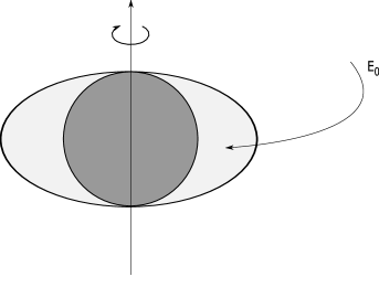
Let us start by recalling that for the stationary Kerr metric the asymptotic time translation Killing field becomes spacelike even in a region outside the event horizon. The region outside the horizon where it is spacelike is called the ergoregion, and the surface where it becomes null is called the ergosphere. For a point particle with four momentum propagating in the Kerr geometry, the conserved Killing energy is . For physical particles the Killing energy is positive provided the Killing vector is also future directed and timelike. However, where becomes spacelike, i.e., in the ergoregion, some physical four-momenta can have negative Killing energy. This fact is at the heart of the Penrose process. We depict the Penrose process in figure 2.1. In this process, a particle of energy is sent from outside into the ergoregion of a rotating black hole where it breaks up into two pieces with Killing energies and . The total energy is conserved , but the energy is arranged to be negative. The particle with energy comes out whereas the particle with energy falls into the black hole. As a result, ; more energy comes out than entered. The black hole absorbs the negative energy and hence loses mass. It also loses angular momentum. In the Penrose process the area of the horizon either increases or remains unchanged.

A very similar phenomenon occurs for a classical field scattering from a rotating black hole spacetime. A scattering in which a wave-packet of more energy than the one sent-in comes out is called a superradiant scattering. This is similar to the lasing action111In chapter 4 we will see that the superradiant scattering is exactly the lasing action when interpreted in the CFT language.. The analogy with lasers immediately suggests that the amplification of the energy of the wave-packet is stimulated emission of quanta from the rotating black hole. Thus, it is expected that quantum fields exhibit not only stimulated emission but also spontaneous emission in a rotating black hole spacetime; though the spontaneous emission is not captured in the classical description of the scattering. Hawking in his pioneering work showed that spontaneous quantum emission occurs even in a non-rotating black hole spacetime222A history of these developments can be found in, e.g., [9].. This phenomenon is called the Hawking effect. It is a pair creation process in which one particle of the pair has negative energy and it falls inside the horizon, while the other particle has positive energy and it stays outside and escapes to infinity. The Hawking radiation comes out with a thermal spectrum at the temperature . We review the Hawking effect in more detail in the next section. In the following we work with Planck units: .
2.2 Hawking Radiation
Hawking in his pioneering work [10] showed that black holes spontaneously emit thermal radiation. In this section we rederive Hawking’s result. Our derivation closely follows the one given in [7, 11]. See also [8, 12, 13, 14].
2.2.1 Quantum Field Theory in Curved Spacetime
We start with a brief review of some basic concepts related to quantum fields in curved spacetime. Let us consider a free massless scalar field on a curved background satisfying the Klein-Gordon equation
| (2.2.1) |
For a solution of this equation we define the conjugate momenta as , where is the vector normal to a Cauchy surface . If and are two solutions to the Klein-Gordon equation, we define the Klein-Gordon inner product as
| (2.2.2) | |||||
This inner product is conserved on-shell but is not positive definite.
One can now choose a complete set of solutions of the Klein-Gordon equation (here is a generalized index which would be momentum in flat spacetime) normalized as
| (2.2.3) |
We now expand the field in this complete basis as
| (2.2.4) |
with being the measure used in the normalization of the delta functions The coefficients in the expansion (2.2.4) can be extracted using the inner product
| (2.2.5) |
To canonically quantize the scalar field we simply write the equal time commutation relation
| (2.2.6) |
This commutation relation leads to the mode algebra
| (2.2.7) |
As in standard quantum mechanics, we define the Fock vacuum for the -basis as the state annihilated by all annihilation operators
| (2.2.8) |
Excited states are obtained by acting with the creation operators on the vacuum . The number of particles in an excited state is the eigenvalue of the number operator .
One can also consider a different complete set of solutions normalized in the same way and expand in terms of this set with annhilation and creation operators . The vacuum with respect to the -modes is defined as
| (2.2.9) |
and in general
| (2.2.10) |
Expansion of a -mode in terms of the -basis takes the following form
| (2.2.11) |
where are the so-called Bogoliubov coefficients. They obey
| (2.2.12) |
From these relations we get
| (2.2.13) |
and
| (2.2.14) |
Thus, the Fock vacuum is in general populated with the -modes. Similarly, the Fock vacuum is populated with the -modes.
Different choices for the complete set of solutions for the Klein-Gordon equation correspond to different choices of the observer. It is easy to verify that in flat spacetime the vacuum states for all inertial observers are the same. However, the vacuum states for a uniformly accelerated observer and an inertial observer are not the same. A uniformly accelerated observer sees the vacuum state of an inertial observer in thermal equilibrium at a non-zero temperature [15]. This is known as the Unruh effect.
Let us emphasize that in a general curved spacetime there is no preferred set of solutions , and hence there is no natural choice for the vacuum state. As a consequence, there is no natural notion of particles. However, in stationary spacetimes the notion of particles is physically and mathematically well defined. If the spacetime admits a globally well defined timelike Killing vector with its norm bounded away from zero, then there are distinguished modes of positive (and negative) frequencies whose Lie derivative along the Killing vector obey
| (2.2.15) |
The analysis presented above is at the heart of the Hawking effect as we review now. By looking at the infalling vacuum in terms of the outgoing modes at late times it leads us to conclude that black holes radiate with a thermal spectrum.
2.2.2 Hawking Radiation
For the Schwarzschild black hole
| (2.2.16) |
we study the Hawking effect by looking at the s-wave of a scalar field in the black-hole background. Since we are working with the s-wave, from now on we restrict our attention to only the temporal and radial part of the metric. To solve the Klein-Gordon equation in the Schwarzschild background we take the ansatz
| (2.2.17) |
which gives the wave equation
| (2.2.18) |
where
| (2.2.19) |
The tortoise radial coordinate is defined as
| (2.2.20) |
Next, we define the null coordinates
| (2.2.21) |
and the conformally related Kruskal coordinates as
| (2.2.22) |
where is the surface gravity of the Schwarzschild black hole. Note that the potential (2.2.19) goes to zero near the horizon and also near infinity . Thus in these two regions we have the positive frequency solutions as
| (2.2.23) |
Our strategy to see the Hawking effect is to look at the infalling vacuum and study how it looks in terms of the outgoing modes at late times in a collapsing black hole spacetime. This is most easily done by looking at the ‘time reversed’ situation, that is, by propagating outgoing waves backward in time and studying their decomposition in terms of ingoing positive and negative frequency modes at past null infinity. To this end let us start by looking at the Penrose diagram in figure 2.2 of a black hole formed in a gravitational collapse.

Notice from equation (2.2.23) that at late times, , the phase of the outgoing modes oscillate rapidly. Therefore geometrical optics approximation is valid, and it becomes better and better as . Outgoing waves propagated backwards starting from all end up on . This is illustrated in figure 2.2. The approximate waveform on can be obtained as follows.
It can be easily shown that at late times near the future null infinity the metric is
| (2.2.24) |
So is the affine parameter and we get
| (2.2.25) |
From figure 2.2 we see that the horizon is at . By definition this is the last ray which makes it out of the black hole. We trace back this ray to past null infinity. We call this ray . We define to be the point where intersects . The metric at past null infinity is
| (2.2.26) |
so the affine parameter is simply . Now recall that the behavior of geodesics sufficiently close to will be well described by the geodesic deviation vector. The geodesic deviation vector describing geodesics near propagates linearly along . As a result, we see that the wave-form near will behave as a function of in the same way as it behaves as a function of the affine parameter along the geodesic tangent to the geodesic deviation vector at any other point on . In particular, we can choose that point to be near at future null infinity. Thus the projection of the wave-form at future null infinity onto past null infinity is given by
| (2.2.27) |
Now we want to express these (projected) outgoing modes in terms of ingoing modes on past null infinity
| (2.2.28) |
Instead of directly evaluating this we look for Fourier modes of (2.2.27)
| (2.2.29) |
This integral can be explicitly evaluated. Keeping we can see that (for details see e.g. Appendix A of [16]) .
| (2.2.30) |
From this is follows that
| (2.2.31) |
Using (2.2.12), (2.2.13) and (2.2.31) one finds
| (2.2.32) |
In arriving at this expression we have replaced on the right hand side by the large time cutoff [17]. The total number of particles emitted is therefore infinite. However this infinity is because the black hole radiates for an infinite amount of time. In this calculation the mass decrease of the black hole because of the radiation is not taken into account. Looking at the number of particles emitted per unit time in the frequency range and we see that the black hole radiates at the temperature
| (2.2.33) |
One can see from the potential (2.2.19) that there is a potential barrier centered around . Thus only a fraction of the flux passes through the barrier. Taking this into account [18] as well as the effect of different angular momenta the total luminosity is given by
| (2.2.34) |
where are the so-called ‘greybody factors.’ They encode the deviation from the blackbody spectrum. They are the fraction of the incoming quanta that fall into the black hole. They are also the fraction of the outgoing quanta emitted at the horizon that make it out to the asymptotic region. We will explicitly calculate these factors for the string theory D1-D5 black holes in section 4.1.2.
We can now estimate the lifetime of a black hole by ignoring the greybody factors and using the Stefan-Boltzman law
| (2.2.35) |
This gives the lifetime
| (2.2.36) |
Observe that the black hole completely evaporates away after a long but finite time.
For rotating black holes almost the same analysis goes through. The most important modification arises from the fact that the Killing vector normal to the horizon is rather than simply , where is the angular velocity of the horizon. This essentially has the effect of the replacement to in (2.2.34). Here is the azimuthal number of the outgoing wave at . The expression for luminosity now reads
| (2.2.37) |
For the integrand is negative; though the equation formally continues to hold. Modes for which are called superradiant modes. For these modes the scattering cross-section is negative. As a result, a wave analogue of the Penrose process occurs. The phenomenon is called superradiance.
A different kind of radiation happens for rotating stars with ergoregions. In this case there is no horizon but a rotating star suffers from a classical instability called the ergoregion instability [19, 20]. Radiation comes out of the star with amplitude increasing exponentially with time. We will see in the later chapters that these seemingly unrelated phenomena, namely, Hawking radiation, superradiance, and ergoregion emission are in fact intimately interrelated.
2.3 Hawking Information Paradox
Hawking’s discovery of the black hole radiance eluded to a deep connection between thermodynamics, gravitational physics, and quantum mechanics. Of particular importance is the formula for the (intrinsic) Bekenstein-Hawking entropy for a black hole
| (2.3.1) |
where is the area of the event horizon in Plank units. The precise nature of the Bekenstein-Hawking entropy has been a topic of intense research since Hawking’s remarkable discovery. Developments in string theory have provided significant insights into the nature of this entropy.
Black hole radiance, at the same time, raises some serious puzzles. These puzzles have been much debated over the last four decades, and many of them have not yet been completely resolved. One of the most debated puzzle of this nature is the Hawking’s proposal that the usual rules of quantum mechanics do not apply to a process in which black holes form and evaporate completely. If this proposal is correct, then we face the formidable task of reformulating quantum physics as a new self-consistent framework that agrees with experiment. To begin with one might be inclined to dismiss Hawking’s proposal—one might argue that the proposal is founded on a semiclassical calculation in which gravitational back reaction effects are not properly taken into account. There is little prospect that a detailed calculation of back reaction effects can be done in the near future, as it would require the knowledge of quantum gravity (see [12] for a more detailed discussion of these issues). On the other hand, it has been argued that Hawking’s conclusion is completely robust and inescapable [21, 22].
The Paradox
As we discussed above, in the semiclassical calculation of black hole radiance, Hawking found that the emitted radiation is exactly thermal. In particular, the details of the radiation do not depend on the nature of the body that collapsed to form the black hole. The state of the radiation is completely determined by the geometry outside the horizon. The fact that the radiation outside the horizon is thermal (and hence a mixed state) is not puzzling. This is because the region outside the horizon is only a part of the full quantum system. The full quantum system consists of the infalling matter and degrees of freedom of quantum fields inside and outside the horizon. The degrees of freedom of quantum fields living outside and inside the horizon are correlated. However neither of them are correlated with the infalling matter. These correlations are responsible for the mixed nature of the radiation observed by observers outside the horizon.
A truly paradoxical situation arises when the black hole evaporates completely; since now the radiation is the complete system, and there is no region behind the horizon. So, if the radiation is indeed in a thermal state as Hawking found, it appears that the initial pure quantum state, by collapsing into a black hole and evaporating completely, evolves in a thermal (mixed) state. This is the Hawking information paradox. In analyzing the evolution of black holes within the standard framework of general relativity and quantum mechanics we are led to conclude that a pure state can evolve into a mixed state. Such an evolution is forbidden by the usual rules of quantum mechanics.
Chapter 3 Fuzzballs
As discussed in the previous chapter, black holes have entropy and they decay with a thermal spectrum. This leads to several puzzles, in particular, to the following, all of which have been intense topics of research in the last four decades:
-
•
What are the microstates of a black hole?
-
•
Where are the microstates of a black hole?
-
•
Does unitarity indeed break down in processes in which black holes form and evaporate completely?
String theory has provided significant insights in answering the first question. For a variety of extremal and near-extremal black holes several authors have counted states at weak coupling using brane physics and have reproduced the Bekenstein-Hawking entropy of corresponding black holes. However these state countings do not tell us anything about how the microstates look like in the strong coupling description, and in particular, in the gravity description. These calculations also do not tell us much about the second and the third question. In the rest of the review an approach to resolve these questions in the framework of the so-called Fuzzball Proposal is discussed. According to this proposal, a black hole geometry is an effective description of an ensemble of states. In the framework of this proposal, quantum gravity effects are not confined to the Planck length. Typical states of the ensemble have structure up to the scale of the horizon. In this proposal, radiation from non-extremal would-be black holes does not happen by a pair production process from the vacuum, but rather happens from the surfaces of the black hole’s microstates. Consequently, the emitted radiation is capable of carrying information, and seemingly the information paradox does not arise.
The fuzzball proposal has met with most success in the case of the two-charge string-theory black holes. For the two charge system all states have been identified in the gravity description and it is shown that typical states have a size that scales as a function of charges as it would for a would-be black hole. For three and four-charge string theory black holes large classes of smooth supersymmetric geometries (see [23, 24, 25, 26] for reviews) and some non-supersymmetric geometries [27, 28, 29, 30, 31] have been constructed. Not all smooth supergravity states have been found. It has been argued that all states may not admit a supergravity description [26]. In this chapter we give a brief overview of the two- and three-charge solutions. In the three-charge case our discussion is particularly brief; many topics of current interest are not addressed.
3.1 Two Charge Solutions
The simplest and the best understood example of quantum gravity effects scaling over distances much bigger than the Planck length is the two-charge system. The black hole solution is obtained by compactifying type IIB string theory on and wrapping D5 branes on the torus and the circle and D1 branes on the circle. The volume of the torus is taken to be and the the length of is taken to be . At low energies the worldvolume dynamics of the branes is described by an super-conformal field theory (SCFT). This SCFT is discussed in section 4.2.1. Here we focus primarily on the supergravity solutions of the system.
Naively the metric and the dilaton are obtained by the Harmonic superposition rule
| (3.1.1) |
For simplicity we have not presented the RR gauge fields produced by the D-branes. The charge radii and are related to integer charges as
| (3.1.2) |
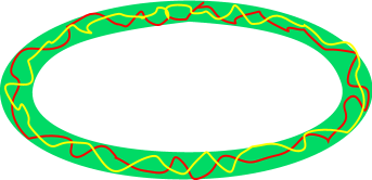
This system has a zero size horizon at . Thus its Bekenstein-Hawking entropy is zero. It was argued in [32] that the metric (3.1.1) is not the correct description for the D1-D5 system. The correct description of the system depends on a closed curve in the non-compact space. The statistical mechanics of this curve gives the transverse size for a typical curve and this sets the size for a typical solution as shown in figure 3.1. A subset of these solutions based on these curves were constructed in [32, 33] and the rest of the solutions were constructed in [34, 35, 36].
We can understand the statistical mechanics of this system by going to a dual frame where the D5 branes map to a fundamental string wrapping and the D1 branes map to momentum running along . The bound state of this system consists of a long string of winding on carrying units of momentum. The momentum manifests itself as bosons and fermions on the string worldsheet. There are 8 such bosons and 8 such fermions corresponding to the string bending in the and directions. Thus the system is a dimensional gas and from its statistical mechanics (see [37] for a recent discussion) it follows that the entropy is
| (3.1.3) |
The generic quanta is in the harmonic
| (3.1.4) |
with occupation
| (3.1.5) |
Now we have a puzzle. The weak coupling F1-P analysis shows that the system has an entropy that scales as . Since the system is supersymmetric, this quantity should be protected by supersymmetry as we increase the string coupling. However, the Bekenstein-Hawking entropy of the naive solution is zero.
The answer to this puzzle lies in the fact that the fundamental string carries only transverse vibrations. This leads to a puffing up of the naive solution. Supergravity solutions for fundamental string carrying vibrations with an arbitrary transverse vibration profile were explicitly constructed in [38, 39]. These solutions correspond to bosonic excitations carrying momentum on a string in the direction. They were dualized to the D1-D5 frame in [32] to get the solutions
| (3.1.6) |
where is taken with respect to the flat metric for the non-compact space. The length of integration is given by
| (3.1.7) |
and the charges are related by
| (3.1.8) |
For these solutions we see that if is bounded from above, that is, if , then at large distances, , we recover the naive metric 3.1.1. Near , metrics for different profile functions differ from each other. Furthermore, all these metrics seem to have a singularity at , but it was shown in [34] that this is just a coordinate artifact; the solutions are completely smooth everywhere. These solutions were quantized using geometric quantization in [40] and were found to give the entropy
| (3.1.9) |
which is the correct contribution, when we take only four bosons into account in the microscopic counting. It is expected that geometric quantization of the full class of solutions constructed in [34, 35, 36] would give the entropy matching with the weak coupling result (3.1.3).

There is another intuitive way of understanding the entropy of these solutions. One puts a ‘stretched horizon’ at where the generic solutions starts to differ from each other. The scale was found in [41]. It was obtained using the fact that in the F1-P frame the string oscillates transverse to itself on the scale of the string length . The dualities map this scale in the D1-D5 frame to
| (3.1.10) |
The area of the stretched horizon is most easily calculated in six dimensions. This is because in six dimensions the Einstein and the string frame metrics are the same. The area is then found to be
| (3.1.11) |
where we have assumed which is true in the classical limit. The six dimensional Newton’s constant is
| (3.1.12) |
The Bekenstein-Hawking entropy of the stretched horizon is therefore
| (3.1.13) |
The above analysis can be extended to the D1-D5 system with angular momentum. We let the angular momentum be in the plane and of the order . The statistical mechanics of the system shows that excitations on the string splits into two parts [37]: (a) all the angular momentum is carried in the lowest harmonic, with this subsystem contributing no entropy, and (b) the rest of the energy is carried by a thermal distribution of excitation in higher harmonics. The entropy of the system is given by
| (3.1.14) |
with the generic quanta in the mode
| (3.1.15) |
with occupation number
| (3.1.16) |
The profile function for this system is given by [41]
| (3.1.17) |
where
| (3.1.18) |
Thus, all geometries described by these profile functions look essentially the same outside a donut shaped region. The Bekenstein-Hawking entropy for the stretched horizon over this donut-shaped region is found to be
| (3.1.19) |


The fact that the real solutions of the D1-D5 system have a size which scales as suggests that probes with insufficient precision fail to capture the details of the system. The intuitive picture that the coarse graining of geometries gives a black hole (or a black ring for sufficiently large angular momentum) was put on a firmer technical footing in references [42, 37, 43, 44, 45, 36, 46, 47] for this system.
All these geometries have an inner region that is asymptotically . As a result, we can have a description of the system in terms of a dual conformal field theory. For the circular profile function [48, 49]
| (3.1.20) |
it was shown in [50] that a minimal scalar falling into the throat takes the time to emerge. This time matches the CFT travel time for the state dual to this geometry. If instead one uses the distribution (3.1.4) for the CFT state one obtains a travel time to be [37]. In the classical limit of large we see that a particle falling-in never emerges back. This suggests that typical states of the D1-D5 system behave like a black hole in the classical limit.
3.2 Three Charge Solutions
Now we present a very brief introduction to three charge solutions. This section is meant to be a starting tutorial on the subject. Many important topics of current interest are not addressed, and none of the three-charge solutions are discussed in detail. The aim here is to provide a flavor of the intense research program that is currently underway to see to what extent the correspondence between D1-D5 states and the smooth bulk solutions extends to the D1-D5-P system. In this section we primarily work in the M-theory frame. Results can be readily dualized to the IIB frame. Our presentation closely follows [23]. See also [24, 25, 26].
A detailed probe analysis of the three-charge system based on the DBI action strongly suggests the existence of a large number of BPS supergravity configurations with the same supersymmetries as the three charge black hole. At the outset the set of configurations suggested by the DBI analysis is so large that finding the corresponding supergravity solutions appears to be a formidable task. Fortunately, it turns out that the entire problem of finding all these BPS configurations reduces to a linear problem in four dimensional Euclidean electrodynamics [51, 52]. It is one of those instances where supersymmetry plays a crucial role in simplifying the problem.
3.2.1 Supersymmetric Configurations
Let us start with M-theory compactified on a six-torus and wrapping three sets of extremal M2 branes on three orthogonal two-tori in the . This configuration is BPS. Rather surprisingly, one can further add three sets of M5 branes on top of this configuration and find configurations that preserve the same set of supersymmetries as the original set of M2 branes [53, 52]. Each set of M5 branes can be thought of as the dual to a set of M2 branes. In each such pair the set of M5 branes wrap the four torus orthogonal to the two torus wrapped by the set of M2 branes. The fifth direction of the M5 branes wrap a contractible spacelike curve (denoted ) in the five-dimensional space orthogonal to . This configuration is summarized in the following table.
| (3.2.8) |
It is argued in [52] that this is the most general supersymmetric configuration that has the same supersymmetries as the original three charge (M2-M2-M2) black hole. (Of course one can consider a configuration with multiple curves and black hole sources, which also has the same supersymmetries as the three charge black hole.) The eleven dimensional metric corresponding to these brane configurations takes the form
| (3.2.9) | |||||
where the five-dimensional space is
| (3.2.10) |
and are the six torus directions. The one form is defined on the spatial section of the five-dimensional metric. Supersymmetry requires that the metric be hyper-Kähler. Two important examples of hyper-Kähler metrics are , multi-centered Taub-NUT metrics. In this review we are only concerned with these two hyper-Kähler manifolds, and their ambipolar generalizations, which we discuss below.
The eleven-dimensional three-form is given by
| (3.2.11) |
The ’s for are three abelian one-forms in the five-dimensional spacetime. We define
| (3.2.12) |
Then the following set of “sequentially linear” BPS equations determine the most general supersymmetric configuration [52]:
| (3.2.13) | |||||
| (3.2.14) | |||||
| (3.2.15) |
where is the Hodge dual taken with respect to the four dimensional hyper-Kähler base and . This system of equation is called “sequentially linear” because if these equations are solved in the order they are presented then at each step one is solving a linear problem.
Supersymmetric Black Ring
As an illustration of the formalism presented above, now we very briefly discuss the supersymmetric black ring solution that can be constructed by solving the BPS equations. We work with flat base space . One starts by choosing the circular profile for the M5 branes in the five-dimensional spacetime that sources ’s. Then one has some freedom in choosing harmonic functions in the solution that add sources for the M2 branes. Finally, with these sources one solves for the one-form . The best coordinate system to solve these equations in this setting is the black ring coordinates. Here we do not review these coordinates. For details of the coordinate system we refer the reader to [54, 23] or to the original references [55, 56]. In black ring coordinates the flat metric has the form
| (3.2.16) |
where , and the ring is located at . The self-dual field strengths (with the orientation ) sourced by the ring are
| (3.2.17) |
where ’s are directly related to the number of wrapped M5 branes. The warp factors take the form
| (3.2.18) |
and the one-form is
| (3.2.19) |
where
| (3.2.20) |
’s are directly related to the number of M2 branes. For a detailed study of physical properties of this solution we refer the reader to original references [57, 53, 52, 58, 59] and to the reviews [54, 23].
3.2.2 Gibbons-Hawking Base
In section 3.2.1 we mentioned that supersymmetry requires us to take the base space metric to be a four-dimensional hyper-Kähler manifold. Flat Euclidean space is the simplest example of a hyper-Kähler manifold. Then there are the multi-centered Gibbons-Hawking (GH) metrics. In this section we briefly review the GH metrics and there ‘ambipolar’ generalizations. Our presentation closely follows [23]. GH metrics have a form of a fibrations over a three dimensional Euclidean flat space :
| (3.2.21) |
where . The function appearing in the metric is a harmonic function on . We take it to have a finite set of isolated sources. The connection is determined via through the equation
| (3.2.22) |
Let be the position of the point sources for the function in the three dimensional base and let , then
| (3.2.23) |
Note that close to a GH center the fuction behaves as Thus, to ensure that the metric is positive definite everywhere on the manifold one usually takes We relax this assumption. In considering negative GH charges we are allowing the base space to flip the signature from to in certain regions. Following [23] we call such metrics ambipolar. At first sight these metrics may look completely unphysical, but this is not the case. Negative definite regions do not lead to any pathological features in the full five-dimensional spacetime [60, 61]. The ambipolar metrics, on the other hand, allow us to to construct explicit BPS solutions with extremely rich physics.
Next, we now introduce a set of frames for the GH base and the two-forms
| (3.2.24) | |||||
| (3.2.25) | |||||
| (3.2.26) |
The two-forms are self-dual and can be used to construct harmonic fluxes as follows
| (3.2.27) |
The two-forms are closed if and only if ’s are harmonic functions on .
3.2.3 Solutions on a Gibbons-Hawking Base
Having discussed elementary properties of GH spaces, we are in the position to solve the BPS equations with a GH base. The first step is to construct the three self-dual two-forms . This is done by introducing three harmonic functions on through (3.2.27). The next step is to substitute these two-forms in the equations for . Solving these equations one finds
| (3.2.28) |
where are three more independent harmonic functions. We now write the one-form as:
| (3.2.29) |
where is solved to be
| (3.2.30) |
and where is another harmonic function on . is a one-form on . Using one can find as a solution of the equation
| (3.2.31) |
Since and are all harmonic, the above equation can be integrated to find and thereby obtaining the complete solution. The full solution is characterized by eight harmonic functions on :
At this point is is worth pointing out that there is a ‘gauge’ invariance in the system of equations related to the fact that for arbitrary constants the shift
| (3.2.32) |
does not change the self-dual two forms (3.2.27). Due to this gauge freedom the solutions are in effect characterized by seven independent harmonic functions. This functional freedom matches with the DBI analysis of [62].
3.2.4 Bubbled Geometries
One of the main purpose of this program is to be able to construct such smooth horizonless BPS configurations with no sources. We now say a few words about smooth geometries. First recall that the black ring solution discussed above has brane sources. Geometries with no brane sources are topologically non-trivial. One of the simplest example of such a configuration is obtained by choosing the GH base with three co-linear centers with charges , where is an integer. This three-center GH space contains three topologically non-trivial two cycles. These cycles can be defined by considering a curve between any two GH centers and considering the fibre along that curve. At the GH centers the fibre shrinks to zero size. As a result, the curve together with the fibre sweeps out a two-cycle. These non-trivial two-cycles are responsible for the bubbling nature of the five-dimensional solutions. In the limit when the GH center is moved on top of the GH center with charge, the corresponding five dimensional geometries reduce to the geometries constructed in [63, 64, 65, 66, 67].
The bubbled geometries with three co-linear centers with GH charges can be thought of as the geometric transition of a zero-entropy black ring. The picture is as follows [60, 61]: We can think of as a trivial GH base with . Now consider taking the black ring in the parameter regime where its entropy decreases and eventually approaches zero. The zero entropy black ring in such a limit is singular, but the singularity is not a curvature singularity. The singularity is a “null orbifold” singularity. In the transitioned geometry the singularity is resolved by the nucleation of two equal, oppositely charged, GH centers . The transitioned geometry has no brane sources. Since in the resolved geometries negative GH centers play a crucial role, ambipolar generalization of GH metrics becomes indispensable. Using the formalism outlined above harmonic functions for the bubbling solutions can be calculated [60, 61]. These solutions have extremely rich physics, and a detailed study of their properties will take us far beyond the scope of this review. We refer the interested reader for more details to the following literature [60, 61, 68, 69, 70, 71, 72, 73, 74, 75, 76, 77, 78, 79, 80, 81, 82, 83, 84, 85, 86, 87, 88].
Chapter 4 Emission From the D1-D5 System
In previous chapter we saw how quantum gravity effects are not confined to the Planck length. In particular, for the two-charge system we explicitly saw how typical fuzzballs extend up to the horizon scale. A similar picture is expected to arise for the three-charge system. This builds up the picture of a black hole being an effective coarse grained geometry. In this chapter we will see an additional process that supports this idea. Here we understand the nature of Hawking radiation by studying emission from the D1-D5 system. The main aim is to understand the interaction between excitations on the inner asymptotically AdS space and excitations on outer flat space from the CFT point of view.
In the CFT analysis, the D1-D5-P black hole is dual to a density matrix (or a thermal state). On the other hand, microstates of the black hole are dual to pure states, and, in particular the special non-extremal fuzzballs of reference [27] are dual to pure states. From the CFT analysis it will become clear that there is no qualitative difference between emission from a thermal state and a pure state. The process dual to emission from a thermal state is Hawking radiation (and superradiance for rotating black holes) that happens in the presence of horizons, while the process dual to emission from the special non-extremal fuzzballs manifests itself as ergoregion emission that happens in the absence of horizons. The classical instability in ergoregion emissions found in [89] is seen to come from Bose-enhancement of quanta collecting in the cap of the highly symmetric fuzzball of reference [27].
The study of emission from brane systems has been spread over several years. Here we give a brief account of the milestones and hope the references we miss can be found in the ones we provide. The emission of minimal scalars from the D1-D5 system without angular momentum was studied in [90, 91, 92, 93, 94, 95]. The emission of minimal scalars with angular momenta was studied in [96, 97]. Universal dynamics of rotating black holes was studied in [98] while the specifics to the D1-D5-P black hole were studied in [99]. These results matched with the corresponding CFT results up to an overall constant. This constant was fixed for s-wave emission in [100] and for higher partial waves in [101] using the AdS/CFT correspondence. Emission of fixed scalars were studied in [100, 102]. Emission from three-branes was studied in [103] while that from extremal Kerr solutions was studied in [104]. Emission from non-extremal fuzzball solutions found in [27] were studied in [89, 105, 101, 106, 107, 108].
This chapter is divided into two parts. The first part explains Hawking radiation, super-radiance, and ergoregion emission for the D1-D5 system from a gravitational or strong coupling point of view. Here the physics looks quite different for the black hole emissions and for the capped geometry emissions. In the second part we rederive these three emissions from the CFT point of view and show that all these emissions are in-fact only different manifestations of the same process.
4.1 Emissions: Gravity Analysis
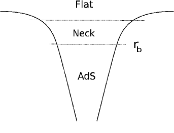
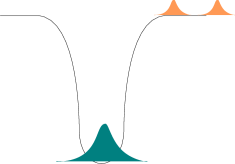
We first review the supergravity D1-D5-P black hole [109, 110] and the non-extremal family of fuzzballs constructed in [27]. We show how the solutions simplify in the decoupling limit into an outer flat space region and and an inner region which is asymptotically AdS space. This is schematically shown in figure 4.1.

We look at the emission of minimally coupled scalars in these backgrounds111An example of a minimally coupled scalar in these backgrounds is a mixture of the dilaton and the graviton with both indices in the direction: .. For the black hole we first calculate the probability for the absorption of a minimal scalar. The emission rate is then related to the absorption probability by detailed balance. This gives us the emission rate as a function of frequency, momentum along , and angular momenta. We use spectral flow to relate this result to superradiance. Then we will look at the emission from the non-extremal fuzzballs. This results in a discrete spectrum and a classical instability.
4.1.1 Gravity Solutions: Black Holes and Smooth Solutions
The supergravity D1-D5-P black hole solution was found in [109, 110] and a non-extremal family of fuzzballs was constructed in [27]. A cartoon of these geometries is shown in figure 4.1. In both cases there is an inner (throat) region, an outer region, and a neck region that joins the inner and the outer regions. The inner region ends up in a horizon in the black hole case, and has smooth cap in the case of fuzzballs. It turns out that the physics is much cleaner if we work in the near-decoupling limit. The solutions and their decoupling limits are discussed in detail in appendix A.
The outer region metric is flat both in the case of the black hole and in the case of the capped geometries. It is simply given by
| (4.1.1) |
The inner region is analyzed separately for the two cases.
D1-D5-P Black Hole
For the black hole the inner region metric is BTZ times an . The is fibered over the BTZ when angular momenta are present. This geometry has been extensively studied in [111]. The metric is given by
| (4.1.2) | |||||
where
| (4.1.3) |
Here the coordinates and are related to the coordinates in the outer flat space as
| (4.1.4) |
and are parameters specifying the geometry. The mass above extremality, momentum charge radius, and angular momenta of the geometry are given as
| (4.1.5) |
The entropy is given by
| (4.1.6) | |||||
while the temperature and the velocity of the horizon along the direction are given by
| (4.1.7) |
Our later expressions will be seen to cleanly split into a left and right sector. So in anticipation we also define a left and a right temperature
| (4.1.8) |
Smooth Solutions
These solutions have a capped inner region. In the decoupling limit they are given by a global AdS with an fibered over it,
Here the coordinate and are related to the coordinates in flat space as
| (4.1.10) |
where
| (4.1.11) |
The non-negative integers parameterize the system. The mass above extremality and charges are given by
| (4.1.12) |
Since this is a smooth geometry without any horizon, it has no Bekenstein-Hawking entropy. The extremal solution found in [48, 49] are obtained by taking while those found in [64, 65] are obtained by taking .
4.1.2 Emission from Black Holes: Hawking Radiation and Superradiance
For the D1-D5-P black hole we first find the absorbtion cross-section for a minimally coupled scalar in this background and the calculate the decay rate using detailed balance. We start by solving the equation
| (4.1.13) |
with purely ingoing boundary conditions at the horizon. It is much simpler to work with a non-rotating black hole first. The results can be very easily generalized to rotating black holes using spectral flow.
Non-Rotating Black Holes: Hawking Radiation
The non-rotating black hole is obtained by simply putting in the metric (A.2). We take as the ansatz for the scalar wave
| (4.1.14) |
with the convention
| (4.1.15) |
Periodicity in the direction restricts to be an integer multiple of .
We now solve for the wave equation in the inner BTZ region and in the outer flat space region separately. We then impose the boundary condition of being purely ingoing at the horizon and match the inner and outer solutions in the neck region. This gives us the probability of absorption that can be related to the cross-section and hence to the decay rate. The angular part of the equation (4.1.13) separates222This is strictly true only in the decoupling limit. To account for the neck region joining the inner and outer region we have to replace where is the parameter that controls the decoupling: . The decoupling limit corresponds to . Further details on this issue can be found in [50, 106]. To keep the notation simple we write explicitly only when we take the strict decoupling limit. and the solutions are simply given by spherical harmonics on . The radial part of the equation becomes
| (4.1.16) |
With the substitution
| (4.1.17) |
the radial equation takes the form
| (4.1.18) |
where
| (4.1.19) |
The solution of this equation with purely ingoing boundary conditions at the horizon is
| (4.1.20) |
The outer region is flat spacetime and the solution of the scalar equation there is
| (4.1.21) |
To find the complete solution we now need to match the above two solutions in the neck region . In the coordinate the neck region is at . Using the asymptotic form of hypergeometric functions, the inner solution in the neck region becomes
| (4.1.22) | |||||
In the neck region the radial coordinate using (4.1.4) becomes
| (4.1.23) |
Using asymptotic form of the Bessel functions, the outer solution in the neck region takes the form
| (4.1.24) | |||||
Matching the two solutions in the neck region gives
| (4.1.25) | |||||
At this point recalling the discussion in footnote 2 and using the identities
| (4.1.26) |
we get
| (4.1.27) |
where
| (4.1.28) |
The outer solution can also be written in terms of the ingoing and outgoing solutions using the appropriate asymptotic behavior of Bessel functions. The result is
| (4.1.29) | |||||
Thus we get the ratio of the outgoing to ingoing flux to be
| (4.1.30) |
The probability for absorption is therefore
| (4.1.31) | |||||
The probability of abosroption is related to the difference between the rates of absorption and emission as
| (4.1.32) |
The minimally coupled scalars being emitted are bosons. Using Bose-Einstein statistics we get the following condition from the detailed balance
| (4.1.33) |
where the and are, for the case of the D1-D5-P black hole, thermal population densities with left and right temperatures and respectively,
| (4.1.34) |
Thus we get the rate of emission in terms of the probability of absorption as
| (4.1.35) | |||||
The probability of absorption is
| (4.1.36) |
The cross section is related to the absorption probability through [97]
| (4.1.37) |
Rotating Black Holes: Superradiance
As promised, now we use the above results to get the emission rate for rotating black holes. This is possible because in the decoupling limit the inner region is an fibered over the BTZ black hole. From the metric (4.1.2) we can see that when we use the transformed coordinates
| (4.1.38) |
with the rest of the coordinates going to themselves, the metric becomes that of BTZ without any fibration, hence that of the inner region of the non-rotating black hole. Under this coordinate transformation the coordinate derivatives transform as
| (4.1.39) |
with the rest of the derivatives going to themselves. Therefore, we simply need to make the change
in the inner solution to get the results for the rotating black hole. This results in
| (4.1.41) | |||||
where
| (4.1.42) | |||||
| (4.1.43) |
From the expression for the probability (4.1.31) and the cross-section (4.1.37) it follows that the cross-section is proportional to
| (4.1.44) |
with a positive proportionality constant. Since , for the non-rotating black hole it is not possible to have a negative cross-section. However, in the case of rotating black holes the cross section can be negative. To look at a much quoted simple case, take the left and right temperatures to be equal and the case of emission of quanta that have no motion along the and directions. Then we get
| (4.1.45) |
which is negative if the scalar wave is co-rotating with the black hole and the emission energy is below a threshold . Thus if a scalar-wave falls on a rotating black hole with the above conditions met, it is reflected back with an increased amplitude. This is the same superradiance as discussed in section 2.1. When we study the microscopics of emission in the next subsection we will see that this is very similar to the lasing action. The superradiant emission happens even at zero temperature [99]. The emission at energies higher than the superradiant bound have a positive cross-section and behave just like Hawking radiation.
4.1.3 Emission from Smooth Solutions with Ergoregions
The emission calculation from smooth solutions with ergoregions is very similar to the one presented above. The main difference is in the boundary conditions. This time we impose regularity in the inner part as there is no horizon and purely outgoing boundary conditions at infinity. We can again first analyze the non-rotating case of . Technically this is not a solution for the D1-D5 system as the fermions have to be periodic on the boundary. However by a coordinate change similar to (4.1.38) the solution can be mapped to D1-D5 solutions.
Following the discussion presented above we first solve the wave equation in the inner region. The angular part of the solution gives us the regular spherical harmonics333 Just like in the black hole case explained in footnote 2 this is strictly true only in the decoupling limit. We take , without explicitely writing so, and take in the end. and the radial part becomes
| (4.1.46) |
Defining the new radial coordinate
| (4.1.47) |
the radial equation becomes
| (4.1.48) |
The solution to this equation that is regular everywhere is
| (4.1.49) |
The outer region is flat so we get the same solution as (4.1.21). Now we match the two solutions in the neck region. In the coordinate, the neck region corresponds to taking the limit . In this limit the inner solution takes the form
| (4.1.50) | |||||
In the neck region the radial coordinate using (4.1.10) becomes
| (4.1.51) |
making the outer solution behave in the neck region in exactly the same way as it does for the black hole case (4.1.24). Matching the two solutions we get
| (4.1.52) |
where
| (4.1.53) |
By imposing purely outgoing boundary conditions on the outer asymptotic solution (4.1.29) and recalling footnote 3 we get
| (4.1.54) |
Thus the matching condition is
| (4.1.55) |
Now recall that, we solved the wave equation by imposing smoothness in the interior and purely outgoing boundary conditions at infinity. Since we have a second order equation and two boundary conditions, solving (4.1.55) gives us a discrete spectrum. We will see that the resulting frequencies have a real and an imaginary part. We solve this using the method of [89]. Since we are looking at we can to zeroth order take the left hand side to be zero. We have two choices
| (4.1.56) |
and
| (4.1.57) |
where is a non-negative integer. Note that the second solution does not make sense as it gives negative frequencies. However, we cannot simply throw it away, because our goal is to look at rotating solutions and right now we are only looking at the non-rotating ones. We will see in a moment that the second solution also gives positive frequencies when we look at rotating geometries by shifting the frequencies in a fashion similar to that described in section 4.1.2. We will also see that even though both choices lead to complex frequencies the first one gives negative imaginary contributions to the frequency. This represents decay of particles piled up in the core region tunneling out of the neck [50, 106]. Although this is a process by which excited D1-D5 systems can decay, it is not a classical instability. The second choice leads to positive imaginary contribution to the frequency which represents an exponential growth in the number of particles outside (as well as inside) [106]. This instability is the ergoregion instability. To get the imaginary part of the frequency we now perturb the solution
| (4.1.58) |
Now we recall footnote 3 and reinstall . We also take , which was shown to be the case in [106]
| (4.1.59) |
We thus get
| (4.1.60) |
and using (4.1.57) we get
| (4.1.61) |
In this equation on the right hand side is understood to be the real part of , . This is because to the leading order is real and is given by (4.1.57).
This gives the rate of increase of the wavefunction. The emission rate is given by
| (4.1.62) |
We translate the results for rotating geometries in a fashion similar to what we did for black holes in section 4.1.2. In the inner region, it corresponds to the shift
| (4.1.63) |
where we have used equations (4.1.12) relating the angular momentum of the special states to integers. The outer region is unaffected by this shift. Thus the emission spectra now becomes
| (4.1.64) | |||||
4.2 Emissions: CFT Analysis
In the previous subsection we saw how the three different kind of emissions from gravitational systems — Hawking radiation and superradiance for black holes and ergoregion emission for rotating stars — are present for the supergravity solutions for the D1-D5 system. Since these geometries have an inner AdS region, we can analyze these emissions from a CFT point of view.
Given the number of examples that confirm the AdS/CFT correspondence, the importance of this calculation can hardly be to get another example of AdS/CFT at work. Instead our aim in this section is to show that in the CFT description the three phenomena mentioned above are the same. If we take our initial state to be a thermal state without R-charge we get the Hawking radiation; if we take to to be a thermal state with an R-charge we get superradiance. If we take the initial state to be a very non-generic state, the one found in [27], the same emission process gives ergoregion instability.
In this subsection we briefly discuss the D1-D5 CFT, the vertex operator responsible for coupling the AdS region to flat space, amplitudes for emissions, spectral flow, and states in CFT involved in the emission processes. For simplicity, we do calculations in the NS-sector instead of in the R-sector. We then find the emission rates from black holes and non-extremal fuzzballs by relating the results to the R-sector by spectral flow.
4.2.1 The D1-D5 CFT
Consider Type IIB string theory compactified on
| (4.2.1) |
and wrap D1 branes on and D5 branes on . The bound states of these branes is described by a field theory. In the limit where the size of is large compared to the size of , and at low energies, excitations live only in the directions. This low energy limit of the field theory flows to a super-conformal field theory living on the circle . A detailed introduction to the CFT and how it arises as a low energy limit of the D1-D5 field theory can be found in [5].
The natural coordinates on the CFT for the time direction and the are the same as the one used for the inner region (4.1.4) and (4.1.10)
| (4.2.2) |
Note that . We also define light cone coordinates as
| (4.2.3) |
It is convenient to euclideanize the time coordinate and work in the coordinates on the complex plane
| (4.2.4) |
It has been conjectured that by varying moduli of string theory one can arrive at the ‘orbifold point’ where the CFT is particularly simple [112, 113, 114]. At the orbifold point the CFT is a 1+1 dimensional sigma model. The base space is spanned by the coordinate and of string theory. The target space of the sigma model is the symmetrized product of copies of ,
| (4.2.5) |
with each copy of the torus giving four bosons and four left and right moving fermions. For the D1-D5 system the fermions are periodic on the .
The R-symmetry group for this CFT is which in the dual picture is related to rotation under . The subscript stands for external as the rotation is in the external space. In addition there is also the (broken) rotation group in the which is . The stands for internal. We use the indices for and and the indices for and respectively.
The four real fermions of the left (right) sector are grouped under two complex fermions () . The bosons are vectors under the and are labeled as .
The superconformal generators are denoted by for the left sector and for the right sector.
Pictorially the CFT is described by a number of component strings of different windings wrapped on the circle . This is shown in figure 4.2. The total winding is . Each component string also has an R-charge of the CFT and is called base spin which is represented by the arrow in the figure. The bosonic and fermionic excitations are represented as arrows running along the strings.

In addition to the operators which can be made from the above field content we also have twist operators denoted by [115, 116, 117, 118]. The ‘n’ gives the order of the twist operator. The action of this operator is as follows: let the order 5 twist operator
| (4.2.6) |
be inserted in the complex plane, then every time one circles the operator the fields of the theory get mapped as
| (4.2.7) |
The other copies of remain unchanged. There is a similar action on fermionic fields. This twisting is schematically depicted in the figure 4.3(a).
The connection between various quantities on the gravity side and on the CFT side is needed for the analysis below. The charge radii and are related with the number of D1 and D5 branes as
| (4.2.8) |
while the five dimensional Newton’s constant is
| (4.2.9) |


The mass above extremality , the momentum charge radius along the and the angular momenta () are related to the left and right dimensions and R-charges through the relations
| (4.2.10) |
We subtracted from the dimensions since this is the dimension of the Ramond sector ground states.
Vertex Operator
We are considering the emission of a minimal scalar with angular quantum numbers . The dimension and charge of the operator dual to this are
| , | |||||
| , | (4.2.11) |
This gets fixed using the AdS/CFT correspondence [119]. Further details on the construction can be found in [101]. We denote the vertex operator for a minimal scalar as
| (4.2.12) |
Spectral Flow
The CFT is naturally defined on the complex plane in the NS sector. However the D1-D5 system is described by the Ramond sector. It turns out that often it is easier to do CFT calculations in the NS sector and relate them to the actual problem by spectral flow [120]. This is like in the gravity analysis where we first calculated quantities for non-rotating geometries and then related to rotating geometries via a coordinate transformation. In fact, the gravity dual to the spectral flow is precisely the coordinate transformation used in the gravity analysis.
4.2.2 States
We want to describe the dual to the black hole geometry and duals to the non-extremal smooth solutions of [27]. In general finding the CFT dual for a smooth geometry is not an easy task, but for geometries of [27] it turns out to be relatively straightforward.
Non-Extremal Fuzzballs
The mass, momentum and angular momenta for these geometries are given in (4.1.12). With the relation (4.2.10) we get the CFT state with
| (4.2.16) |
and similar expressions for the right sector. From the expression for the spectral flow (4.2.14) we see that this state is related by a spectral flow of and units to the state with and . This state is just the vacuum in the NS sector. So we see that there is a unique state with the dimensions and charge given by (4.2.16) given by
| (4.2.17) |
Even though its possible to write down the above state explicitly in the R-sector, the physics and presentation is cleaner if we use the fact that its related to the NS vacuum by spectral flow. The NS vacuum is dual to the global AdS.
For a general amplitude of emission we need to calculate a 3-point function. However, since we spectral flowed the initial state to the NS vacuum we now need to calculate a two point function. This restricts the final states to be of the form
| (4.2.18) |
Equivalently,
| (4.2.19) |
Black Hole
The black hole has an entropy and is thus dual to an ensemble in the CFT. We now show that the entropy and the temperature of the D1-D5-P black hole is invariant under spectral flow. Thus the emission rates of non-rotating black holes with a certain left and right temperature are related by spectral flow to emission rates for rotating black holes with the same left and right temperatures. Additionally we can work in the NS sector and relate the results to the R sector by spectral flow.
The left sector entropy is given by [111]
| (4.2.20) |
and the temperature by
| (4.2.21) |
Using (4.2.14) we see that the left sector entropy and temperature (and similarly right sector entropy and temperature) are invariant under spectral flow.
Since the black hole is a thermal ensemble of pure states we can describe it by a thermal state. This state has the property
| (4.2.22) |
where is the density matrix. In our case the thermal state also has angular momenta and is related by spectral flow to a thermal state wihout any angular momenta via
| (4.2.23) |
where are defined in (4.2.10).
4.2.3 Amplitudes
In [101] it was shown that the amplitude for emission is given as
| (4.2.24) |
where
| (4.2.25) |
The amplitude for absorption is obtained by taking and . For later convenience we now define the light-cone momenta as
| (4.2.26) |
The amplitude in terms of the light-cone momenta and the coordinate takes the form
| (4.2.27) | |||||
where the extra factors of come from the Jacobian of the conformal transformation. We can now use (4.2.15) to express the amplitude in terms of the spectral flowed states (4.2.13) as
| (4.2.28) | |||||
where the spectral flowed left and right light-cone momenta are
| (4.2.29) |
4.2.4 Thermal States: Hawking Radiation and Superradiance
We now want to show how the vertex operator of section 4.2 gives Hawking radiation and superradiance for black holes. In the CFT language black holes correspond to thermal states as described in section 4.2.2. The probability after summing over all final states is given by
| (4.2.30) | |||||
Since the CFT lives on the , we need the thermal two point function on a cylinder. For the states dual to a black hole the entropy is dominated by the long string sector (at least at the orbifold point). Therefore, we can take the spatial direction to be decompactified in the supergravity limit [98]. We then have
| (4.2.31) |
Thus we can now write
| (4.2.32) |
Using the identity
| (4.2.33) |
we get
| (4.2.34) |
From (4.2.23) we see that and . Further using (4.2.29), (4.2.26), (4.2.11) and (4.2.10) we get
| (4.2.35) |
Putting these together we have
| (4.2.36) | |||||
where and are defined as
| (4.2.37) |
Using (4.2.8) and (4.2.9), we immediately see that this matches the gravity answer (4.1.41).
It is instructive to see in more detail why we get an exponential growth of emission for superradiance while not for Hawking radiation. The physics is exactly the same as the lasing action. As the emitted particles are bosons, the net rate of production of bulk quanta is
| (4.2.38) |
For large number of quanta we can approximate . We can get the expression for by taking and in (4.2.28) and hence in (4.2.34). We see that
| (4.2.39) |
where the proportinality constant is positive. For cases when this quantity is positive (superradiance) we get an exponentially growing number of quanta (black hole bomb [122]). When the above is negative we have a steady Hawking radiation.
4.2.5 Special States: Ergoregion Emission
We now evaluate the rate of emission for special states dual to [27]. In particular, we want to calculate
| (4.2.40) |
where normalized states are
| (4.2.41) |
It can be shown that
| (4.2.42) |
Thus we get
| (4.2.43) |
Going back to and coordinates we get
| (4.2.44) | |||||
Squaring to amplitude we get the probability
| (4.2.45) |
where
| (4.2.46) |
Thus we get
| (4.2.47) |
Comparing this result with the gravity answer (4.1.64) and taking into account the fact that is an integer and is the real part of , we see that the two match exactly.
So far we have only gotten the emission rate. This by itself cannot lead to a classical instability. However recall from section 4.2.1 that the target space of the CFT is
| (4.2.48) |
Thus all the states we make have to be symmetrized over all strands. Also the vertex operator has to symmetrized in all its indices and its action should be symmetrized on all strands. We refer the reader to [101, 108] for the computation. The result is that if quanta have already been emitted then we have
| (4.2.49) |
For large this leads to an exponentially growing number of emitted particles. On the gravity side it is interpreted as the classical ergoregion instability [101, 108].
4.3 Understanding the Physics of Emissions
In this section we studied emission from the D1-D5 system from both the gravity and the CFT perspective. We saw that on the gravity side black holes emit Hawking radiation and if they are rotating they also exhibit superradiance. The special non-extremal fuzzballs of reference [27] on the other hand exhibit ergoregion instability. Non-extremal fuzzballs do not have a horizon or singularity and thus have more in common with stars than black holes. On the CFT side we saw that all these emission processes—Hawking radiation, superradiance, and ergoregion instability—are infact different manifestations of the same phenomenon. If the CFT is taken to be in a thermal state with no rotation we get Hawking radiation; if it is taken in a thermal state with rotation (which amounts to having a chemical potential) we get superradiance. For pure states dual to geometries constructed in [27] we get ergoregion instability. Thus from the CFT perspective a unified picture of various emission phenomena emerges. This unification strongly suggests that the D1-D5-P black hole is nothing but an effective description of an ensemble of smooth geometries.
One might wonder if a pure state exhibits a classical instability [89] how can an ensemble not exhibit it. In [123] the authors studied the classical stability of the rotating D1-D5-P black hole. No instabilities were found. We can now understand how this comes about. We first explain this on the CFT side and then propose a picture as to how it might look on the gravity side.


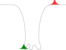
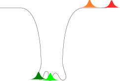
The states dual to the special non-extremal fuzzballs we studied have all the component strings in the same state. We refer to this as the background state. The twist operator then twists of the component strings together during the emission process. In figure 4.4 we show the CFT state after one particle has been emitted. In the large limit this is like a quantum sitting in the background state. The next emission twists a new set of strands together (the process involving the original strings is highly suppressed). This is shown in figure 4.4. Thus after the second emission we have two quanta in the same state. This coherence of these quanta leads to a Bose-enhancement of the emission rate and we get a classical instability.
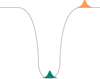
On the gravity side the picture is as follows. The non-extremal fuzzballs all have a core AdS3 region. Global AdS3 has a discrete spectrum with energy levels separated by and the process of emission produces an excitation in this region in a certain harmonic. This is shown in figure 4.5. The second emission causes another excitation in the same harmonic as shown in figure 4.5. The coherence of these quanta in the core AdS region leads to a Bose enhancement and hence to a classical instability.
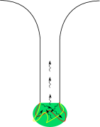
The generic state of the CFT has component strings of different lengths with different excitations. The probability of the second particle being produced in the same state is suppressed by . Thus there is no Bose enhancement and no classical instability. On the gravity side a typical state is expected to have complicated throat structure and hence the energy levels in the throat region will be very close to each other. In figure 4.6 we show a heuristic picture of this. The first emission causes a particle to be produced in one corner of the cap (figure 4.6) and the second emission produces a particle in another corner of the cap (figure 4.6). Thus for a generic fuzzball there will not be any Bose enhancement and hence no classical instability. This is consistent with the results of [123] that the rotating D1-D5-P black holes do not suffer from classical instability.
This suggests a modification of the traditional picture of black hole evaporation. In the traditional picture, shown in figure 4.7, Hawking quanta are produced as pair creation in the vicinity of the black hole. One particle of the pair has negative energy and it falls inside the horizon, while the other particle has positive energy and it stays outside and escapes to infinity. Since such pairs are created out of vacuum fluctuations near the horizon, they do not carry any information about the state that collapsed to form the black hole. The fuzzball proposal modifies this picture. In the fuzzball proposal black holes are effective descriptions of ensemble of fuzzballs. Typical fuzzball states have structure up to the horizon scale as shown in figure 4.7. The analysis of this section suggests that inside a fuzzball different parts continuously exchange quanta; only some of these quanta escape to infinity from the surface of the fuzzball. The average behavior of a typical fuzzball is captured by the corresponding black hole.

Acknowledgements
AV thanks the organizers of the Fifth International Modave Summer School on Mathematical Physics held in Modave, Belgium, August 2009, where the lectures on which these notes are based were given. The work of AV was supported by IISN Belgium conventions 4.4511.06 and 4.4514.08 and by the Belgian Federal Science Policy Office through the Interuniversity Attraction Pole P6/11. The work of BDC was supported by the Foundation for Fundamental Research on Matter (FOM). AV would like to thank Andrea Puhm and Clément Ruef for useful discussions at the summer school. BDC would like to thank Steven G. Avery, Samir D. Mathur and Yogesh K. Srivastava for many useful discussions.
Appendix A D1-D5-P Black Hole
In this appendix we give the explicit metric for the rotating non-extremal D1-D5-P black hole. Explicit metric is needed for certain calculations presented in the main text. Non-extremal fuzzball states of [48, 49, 64, 65, 66, 27] are also closely related to the D1-D5-P black hole. In the following, we discuss relevant properties of the D1-D5-P black hole and some salient features of the non-extremal fuzzballs of [27] . Our presentation follows [109, 110, 27].
Consider type IIB string theory compactified on . Let the volume of be and the length of is . The is described by coordinates and the by a coordinate . The noncompact is described by a time coordinate , a radial coordinate , and angular coordinates . The rotating non-extremal D1-D5-P black hole has angular momenta along , parameterized by . The solution also carries three kinds of charges: units of D1 charge along , units of D5 charge wrapped on , and units of momentum charge (P) along . These charges are parameterized by , respectively. To avoid notational clutter we use the abbreviations
| (A.1) |
The non-extremality of the solution is captured by the parameter . With these preliminaries, we are in position to write the black hole solution of interest:
| (A.2) | |||||
where
| (A.3) |
The dilaton has the profile
| (A.4) |
The D1 and D5 charges of the solution produce a RR two-form gauge field. It is given by [65]
| (A.5) | |||||
The angular momenta are given as
| (A.6) | |||||
| (A.7) |
and the ADM mass is
| (A.8) |
It is convenient to define charge radii
| (A.9) |
Extremal SUSY solutions are reached in the limit
| (A.10) |
whereupon we get the BPS relation
| (A.11) |
The integer charges of the solution are related to the ’s through
| (A.12) | |||||
| (A.13) | |||||
| (A.14) |
We can now see that metric splits into an outer flat space region and an inner ‘core’ region. The core region asymptote to . To see the outer flat region it suffices to take . In this limit we get flat space
| (A.15) |
To see the core part of the geometry we can use the Killing symmetries and to rewrite the metric (A.2) as a fibration of these two directions over a four-dimensional base space [27]. This gives
| (A.16) | |||||
where , .
The near-horizon limit is obtained by assuming that , and focusing on the region . This amounts to taking , , and approximating . This gives us the asymptotically AdS geometry:
| (A.17) | |||||
This can be rewritten as
| (A.18) | |||||
where
| (A.19) |
The coordinates and are related to the coordinates in flat space as
| (A.20) |
In this limit the mass above extremality, momentum, and angular momenta become
| (A.21) |
In [27] non-extremal smooth solutions were constructed from the above black hole solution by taking a limit where the circle shrinks to zero at the larger root of without a conical defect. Each such state has an inner AdS region. The AdS region ends in a smooth cap. In the decoupling limit the metric for these states is given by a global AdS with an fibered over it:
| (A.22) | |||||
The coordinates and are related to the coordinates in flat space as
| (A.23) |
where
| (A.24) |
The non-negative integers parameterize these states. The mass above extremality and various charges are given by
| (A.25) |
Since all these geometries are smooth geometries without horizons they do not have entropy and temperature. Further details can be found in [27].
Bibliography
- [1] A. Sen, Extremal black holes and elementary string states, Mod. Phys. Lett. A10, 2081–2094 (1995) [hep-th/9504147].
- [2] A. Strominger and C. Vafa, Microscopic Origin of the Bekenstein-Hawking Entropy, Phys. Lett. B379, 99–104 (1996) [hep-th/9601029].
- [3] A. W. Peet, The Bekenstein formula and string theory (N-brane theory), Class. Quant. Grav. 15, 3291–3338 (1998) [hep-th/9712253].
- [4] A. W. Peet, TASI lectures on black holes in string theory, hep-th/0008241.
- [5] J. R. David, G. Mandal and S. R. Wadia, Microscopic formulation of black holes in string theory, Phys. Rept. 369, 549–686 (2002) [hep-th/0203048].
- [6] S. D. Mathur, The quantum structure of black holes, Class. Quant. Grav. 23, R115 (2006) [hep-th/0510180].
- [7] R. M. Wald, General Relativity,. Chicago, Usa: Univ. Pr. ( 1984) 491p.
- [8] T. Jacobson, Introduction to quantum fields in curved spacetime and the Hawking effect, gr-qc/0308048.
- [9] D. N. Page, Hawking radiation and black hole thermodynamics, New J. Phys. 7, 203 (2005) [hep-th/0409024].
- [10] S. W. Hawking, Particle Creation by Black Holes, Commun. Math. Phys. 43, 199–220 (1975).
- [11] C. Kiefer, Thermodynamics of black holes and Hawking radiation,. In *Fre, P. (ed.) et al.: Classical and quantum black holes* 19-74.
- [12] R. M. Wald, Quantum field theory in curved space-time and black hole thermodynamics,. Chicago, USA: Univ. Pr. (1994) 205 p.
- [13] J. H. Traschen, An introduction to black hole evaporation, gr-qc/0010055.
- [14] S. F. Ross, Black hole thermodynamics, hep-th/0502195.
- [15] W. G. Unruh, Notes on black hole evaporation, Phys. Rev. D14, 870 (1976).
- [16] R. M. Wald, On Particle Creation by Black Holes, Commun. Math. Phys. 45, 9–34 (1975).
- [17] S. B. Giddings and W. M. Nelson, Quantum emission from two-dimensional black holes, Phys. Rev. D46, 2486–2496 (1992) [hep-th/9204072].
- [18] B. S. DeWitt, Quantum Field Theory in Curved Space-Time, Phys. Rept. 19, 295–357 (1975).
- [19] J. L. Friedman, Ergosphere Instability, Commun. Math. Phys. 63, 243–255 (1978).
- [20] N. Comins and B. F. Schutz, On the ergoregion instability, Proc. R. Soc. A 364, 211–226 (1978).
- [21] S. D. Mathur, What Exactly is the Information Paradox?, Lect. Notes Phys. 769, 3–48 (2009) [0803.2030].
- [22] S. D. Mathur, The information paradox: A pedagogical introduction, Class. Quant. Grav. 26, 224001 (2009) [0909.1038].
- [23] I. Bena and N. P. Warner, Black holes, black rings and their microstates, Lect. Notes Phys. 755, 1–92 (2008) [hep-th/0701216].
- [24] K. Skenderis and M. Taylor, The fuzzball proposal for black holes, Phys. Rept. 467, 117–171 (2008) [0804.0552].
- [25] V. Balasubramanian, J. de Boer, S. El-Showk and I. Messamah, Black Holes as Effective Geometries, Class. Quant. Grav. 25, 214004 (2008) [0811.0263].
- [26] J. de Boer, S. El-Showk, I. Messamah and D. Van den Bleeken, A bound on the entropy of supergravity?, 0906.0011.
- [27] V. Jejjala, O. Madden, S. F. Ross and G. Titchener, Non-supersymmetric smooth geometries and D1-D5-P bound states, Phys. Rev. D71, 124030 (2005) [hep-th/0504181].
- [28] S. Giusto, S. F. Ross and A. Saxena, Non-supersymmetric microstates of the D1-D5-KK system, JHEP 12, 065 (2007) [0708.3845].
- [29] J. H. Al-Alawi and S. F. Ross, Spectral Flow of the Non-Supersymmetric Microstates of the D1-D5-KK System, JHEP 10, 082 (2009) [0908.0417].
- [30] I. Bena, S. Giusto, C. Ruef and N. P. Warner, A (Running) Bolt for New Reasons, JHEP 11, 089 (2009) [0909.2559].
- [31] N. Bobev and C. Ruef, The Nuts and Bolts of Einstein-Maxwell Solutions, 0912.0010.
- [32] O. Lunin and S. D. Mathur, Metric of the multiply wound rotating string, Nucl. Phys. B610, 49–76 (2001) [hep-th/0105136].
- [33] O. Lunin and S. D. Mathur, AdS/CFT duality and the black hole information paradox, Nucl. Phys. B623, 342–394 (2002) [hep-th/0109154].
- [34] O. Lunin, J. M. Maldacena and L. Maoz, Gravity solutions for the D1-D5 system with angular momentum, hep-th/0212210.
- [35] M. Taylor, General 2 charge geometries, JHEP 03, 009 (2006) [hep-th/0507223].
- [36] I. Kanitscheider, K. Skenderis and M. Taylor, Fuzzballs with internal excitations, JHEP 06, 056 (2007) [0704.0690].
- [37] V. Balasubramanian, P. Kraus and M. Shigemori, Massless black holes and black rings as effective geometries of the D1-D5 system, Class. Quant. Grav. 22, 4803–4838 (2005) [hep-th/0508110].
- [38] C. G. Callan, J. M. Maldacena and A. W. Peet, Extremal Black Holes As Fundamental Strings, Nucl. Phys. B475, 645–678 (1996) [hep-th/9510134].
- [39] A. Dabholkar, J. P. Gauntlett, J. A. Harvey and D. Waldram, Strings as Solitons & Black Holes as Strings, Nucl. Phys. B474, 85–121 (1996) [hep-th/9511053].
- [40] V. S. Rychkov, D1-D5 black hole microstate counting from supergravity, JHEP 01, 063 (2006) [hep-th/0512053].
- [41] O. Lunin and S. D. Mathur, Statistical interpretation of Bekenstein entropy for systems with a stretched horizon, Phys. Rev. Lett. 88, 211303 (2002) [hep-th/0202072].
- [42] L. F. Alday, J. de Boer and I. Messamah, The gravitational description of coarse grained microstates, JHEP 12, 063 (2006) [hep-th/0607222].
- [43] S. Giusto, S. D. Mathur and Y. K. Srivastava, Dynamics of supertubes, Nucl. Phys. B754, 233–281 (2006) [hep-th/0510235].
- [44] K. Skenderis and M. Taylor, Fuzzball solutions and D1-D5 microstates, Phys. Rev. Lett. 98, 071601 (2007) [hep-th/0609154].
- [45] I. Kanitscheider, K. Skenderis and M. Taylor, Holographic anatomy of fuzzballs, JHEP 04, 023 (2007) [hep-th/0611171].
- [46] S. D. Mathur, Black hole size and phase space volumes, 0706.3884.
- [47] S. R. Das and G. Mandal, Microstate Dependence of Scattering from the D1-D5 System, JHEP 04, 036 (2009) [0812.1358].
- [48] V. Balasubramanian, J. de Boer, E. Keski-Vakkuri and S. F. Ross, Supersymmetric conical defects: Towards a string theoretic description of black hole formation, Phys. Rev. D64, 064011 (2001) [hep-th/0011217].
- [49] J. M. Maldacena and L. Maoz, De-singularization by rotation, JHEP 12, 055 (2002) [hep-th/0012025].
- [50] O. Lunin and S. D. Mathur, The slowly rotating near extremal D1-D5 system as a ’hot tube’, Nucl. Phys. B615, 285–312 (2001) [hep-th/0107113].
- [51] J. P. Gauntlett, J. B. Gutowski, C. M. Hull, S. Pakis and H. S. Reall, All supersymmetric solutions of minimal supergravity in five dimensions, Class. Quant. Grav. 20, 4587–4634 (2003) [hep-th/0209114].
- [52] I. Bena and N. P. Warner, One ring to rule them all … and in the darkness bind them?, Adv. Theor. Math. Phys. 9, 667–701 (2005) [hep-th/0408106].
- [53] H. Elvang, R. Emparan, D. Mateos and H. S. Reall, Supersymmetric black rings and three-charge supertubes, Phys. Rev. D71, 024033 (2005) [hep-th/0408120].
- [54] R. Emparan and H. S. Reall, Black rings, Class. Quant. Grav. 23, R169 (2006) [hep-th/0608012].
- [55] R. Emparan and H. S. Reall, A rotating black ring in five dimensions, Phys. Rev. Lett. 88, 101101 (2002) [hep-th/0110260].
- [56] R. Emparan and H. S. Reall, Generalized Weyl solutions, Phys. Rev. D65, 084025 (2002) [hep-th/0110258].
- [57] H. Elvang, R. Emparan, D. Mateos and H. S. Reall, A supersymmetric black ring, Phys. Rev. Lett. 93, 211302 (2004) [hep-th/0407065].
- [58] J. P. Gauntlett and J. B. Gutowski, Concentric black rings, Phys. Rev. D71, 025013 (2005) [hep-th/0408010].
- [59] J. P. Gauntlett and J. B. Gutowski, General concentric black rings, Phys. Rev. D71, 045002 (2005) [hep-th/0408122].
- [60] I. Bena and N. P. Warner, Bubbling supertubes and foaming black holes, Phys. Rev. D74, 066001 (2006) [hep-th/0505166].
- [61] P. Berglund, E. G. Gimon and T. S. Levi, Supergravity microstates for BPS black holes and black rings, JHEP 06, 007 (2006) [hep-th/0505167].
- [62] I. Bena and P. Kraus, Three Charge Supertubes and Black Hole Hair, Phys. Rev. D70, 046003 (2004) [hep-th/0402144].
- [63] S. D. Mathur, A. Saxena and Y. K. Srivastava, Constructing ’hair’ for the three charge hole, Nucl. Phys. B680, 415–449 (2004) [hep-th/0311092].
- [64] O. Lunin, Adding momentum to D1-D5 system, JHEP 04, 054 (2004) [hep-th/0404006].
- [65] S. Giusto, S. D. Mathur and A. Saxena, Dual geometries for a set of 3-charge microstates, Nucl. Phys. B701, 357–379 (2004) [hep-th/0405017].
- [66] S. Giusto, S. D. Mathur and A. Saxena, 3-charge geometries and their CFT duals, Nucl. Phys. B710, 425–463 (2005) [hep-th/0406103].
- [67] S. Giusto and S. D. Mathur, Geometry of D1-D5-P bound states, Nucl. Phys. B729, 203–220 (2005) [hep-th/0409067].
- [68] A. Saxena, G. Potvin, S. Giusto and A. W. Peet, Smooth geometries with four charges in four dimensions, JHEP 04, 010 (2006) [hep-th/0509214].
- [69] I. Bena, C.-W. Wang and N. P. Warner, Sliding rings and spinning holes, JHEP 05, 075 (2006) [hep-th/0512157].
- [70] S. Giusto, S. D. Mathur and Y. K. Srivastava, A microstate for the 3-charge black ring, Nucl. Phys. B763, 60–90 (2007) [hep-th/0601193].
- [71] I. Bena, C.-W. Wang and N. P. Warner, The foaming three-charge black hole, Phys. Rev. D75, 124026 (2007) [hep-th/0604110].
- [72] V. Balasubramanian, E. G. Gimon and T. S. Levi, Four Dimensional Black Hole Microstates: From D-branes to Spacetime Foam, JHEP 01, 056 (2008) [hep-th/0606118].
- [73] I. Bena, C.-W. Wang and N. P. Warner, Mergers and Typical Black Hole Microstates, JHEP 11, 042 (2006) [hep-th/0608217].
- [74] M. C. N. Cheng, More bubbling solutions, JHEP 03, 070 (2007) [hep-th/0611156].
- [75] J. Ford, S. Giusto and A. Saxena, A class of BPS time-dependent 3-charge microstates from spectral flow, Nucl. Phys. B790, 258–280 (2008) [hep-th/0612227].
- [76] E. G. Gimon, T. S. Levi and S. F. Ross, Geometry of non-supersymmetric three-charge bound states, JHEP 08, 055 (2007) [0705.1238].
- [77] I. Bena, N. Bobev and N. P. Warner, Bubbles on Manifolds with a U(1) Isometry, JHEP 08, 004 (2007) [0705.3641].
- [78] E. G. Gimon and T. S. Levi, Black Ring Deconstruction, JHEP 04, 098 (2008) [0706.3394].
- [79] I. Bena, C.-W. Wang and N. P. Warner, Plumbing the Abyss: Black Ring Microstates, JHEP 07, 019 (2008) [0706.3786].
- [80] A. Castro, J. L. Davis, P. Kraus and F. Larsen, String Theory Effects on Five-Dimensional Black Hole Physics, Int. J. Mod. Phys. A23, 613–691 (2008) [0801.1863].
- [81] J. de Boer, F. Denef, S. El-Showk, I. Messamah and D. Van den Bleeken, Black hole bound states in , JHEP 11, 050 (2008) [0802.2257].
- [82] I. Bena, N. Bobev and N. P. Warner, Spectral Flow, and the Spectrum of Multi-Center Solutions, Phys. Rev. D77, 125025 (2008) [0803.1203].
- [83] I. Bena, N. Bobev, C. Ruef and N. P. Warner, Entropy Enhancement and Black Hole Microstates, 0804.4487.
- [84] J. Raeymaekers, W. Van Herck, B. Vercnocke and T. Wyder, 5D fuzzball geometries and 4D polar states, JHEP 10, 039 (2008) [0805.3506].
- [85] I. Bena, N. Bobev, C. Ruef and N. P. Warner, Supertubes in Bubbling Backgrounds: Born-Infeld Meets Supergravity, JHEP 07, 106 (2009) [0812.2942].
- [86] I. Bena, S. Giusto, C. Ruef and N. P. Warner, Multi-Center non-BPS Black Holes - the Solution, JHEP 11, 032 (2009) [0908.2121].
- [87] I. Bena, S. Giusto, C. Ruef and N. P. Warner, Supergravity Solutions from Floating Branes, 0910.1860.
- [88] N. Bobev, Spectral flow and multi-centered solutions of supergravity, Nucl. Phys. Proc. Suppl. 192-193, 130–131 (2009).
- [89] V. Cardoso, O. J. C. Dias, J. L. Hovdebo and R. C. Myers, Instability of non-supersymmetric smooth geometries, Phys. Rev. D73, 064031 (2006) [hep-th/0512277].
- [90] C. G. Callan and J. M. Maldacena, D-brane Approach to Black Hole Quantum Mechanics, Nucl. Phys. B472, 591–610 (1996) [hep-th/9602043].
- [91] A. Dhar, G. Mandal and S. R. Wadia, Absorption vs decay of black holes in string theory and T- symmetry, Phys. Lett. B388, 51–59 (1996) [hep-th/9605234].
- [92] S. R. Das and S. D. Mathur, Comparing decay rates for black holes and D-branes, Nucl. Phys. B478, 561–576 (1996) [hep-th/9606185].
- [93] S. R. Das and S. D. Mathur, Interactions involving D-branes, Nucl. Phys. B482, 153–172 (1996) [hep-th/9607149].
- [94] J. M. Maldacena and A. Strominger, Black hole greybody factors and D-brane spectroscopy, Phys. Rev. D55, 861–870 (1997) [hep-th/9609026].
- [95] I. R. Klebanov and S. D. Mathur, Black hole greybody factors and absorption of scalars by effective strings, Nucl. Phys. B500, 115–132 (1997) [hep-th/9701187].
- [96] S. D. Mathur, Absorption of angular momentum by black holes and D- branes, Nucl. Phys. B514, 204–226 (1998) [hep-th/9704156].
- [97] S. S. Gubser, Can the effective string see higher partial waves?, Phys. Rev. D56, 4984–4993 (1997) [hep-th/9704195].
- [98] J. M. Maldacena and A. Strominger, Universal low-energy dynamics for rotating black holes, Phys. Rev. D56, 4975–4983 (1997) [hep-th/9702015].
- [99] O. J. C. Dias, R. Emparan and A. Maccarrone, Microscopic Theory of Black Hole Superradiance, Phys. Rev. D77, 064018 (2008) [0712.0791].
- [100] J. R. David, G. Mandal and S. R. Wadia, Absorption and Hawking radiation of minimal and fixed scalars, and AdS/CFT correspondence, Nucl. Phys. B544, 590–611 (1999) [hep-th/9808168].
- [101] S. G. Avery, B. D. Chowdhury and S. D. Mathur, Emission from the D1D5 CFT, JHEP 10, 065 (2009) [0906.2015].
- [102] C. G. Callan, Jr., S. S. Gubser, I. R. Klebanov and A. A. Tseytlin, Absorption of fixed scalars and the D-brane approach to black holes, Nucl. Phys. B489, 65–94 (1997) [hep-th/9610172].
- [103] S. S. Gubser, I. R. Klebanov and A. A. Tseytlin, String theory and classical absorption by three-branes, Nucl. Phys. B499, 217–240 (1997) [hep-th/9703040].
- [104] I. Bredberg, T. Hartman, W. Song and A. Strominger, Black Hole Superradiance From Kerr/CFT, 0907.3477.
- [105] B. D. Chowdhury and S. D. Mathur, Radiation from the non-extremal fuzzball, Class. Quant. Grav. 25, 135005 (2008) [0711.4817].
- [106] B. D. Chowdhury and S. D. Mathur, Pair creation in non-extremal fuzzball geometries, Class. Quant. Grav. 25, 225021 (2008) [0806.2309].
- [107] B. D. Chowdhury and S. D. Mathur, Non-extremal fuzzballs and ergoregion emission, Class. Quant. Grav. 26, 035006 (2009) [0810.2951].
- [108] S. G. Avery and B. D. Chowdhury, Emission from the D1D5 CFT: Higher Twists, 0907.1663.
- [109] M. Cvetic and D. Youm, General Rotating Five Dimensional Black Holes of Toroidally Compactified Heterotic String, Nucl. Phys. B476, 118–132 (1996) [hep-th/9603100].
- [110] M. Cvetic and F. Larsen, General rotating black holes in string theory: Greybody factors and event horizons, Phys. Rev. D56, 4994–5007 (1997) [hep-th/9705192].
- [111] M. Cvetic and F. Larsen, Near horizon geometry of rotating black holes in five dimensions, Nucl. Phys. B531, 239–255 (1998) [hep-th/9805097].
- [112] N. Seiberg and E. Witten, The D1/D5 system and singular CFT, JHEP 04, 017 (1999) [hep-th/9903224].
- [113] F. Larsen and E. J. Martinec, U(1) charges and moduli in the D1-D5 system, JHEP 06, 019 (1999) [hep-th/9905064].
- [114] J. de Boer, Six-dimensional supergravity on S**3 x AdS(3) and 2d conformal field theory, Nucl. Phys. B548, 139–166 (1999) [hep-th/9806104].
- [115] O. Lunin and S. D. Mathur, Correlation functions for M(N)/S(N) orbifolds, Commun. Math. Phys. 219, 399–442 (2001) [hep-th/0006196].
- [116] O. Lunin and S. D. Mathur, Three-point functions for M(N)/S(N) orbifolds with N = 4 supersymmetry, Commun. Math. Phys. 227, 385–419 (2002) [hep-th/0103169].
- [117] A. Pakman, L. Rastelli and S. S. Razamat, Diagrams for Symmetric Product Orbifolds, JHEP 10, 034 (2009) [0905.3448].
- [118] A. Pakman, L. Rastelli and S. S. Razamat, Extremal Correlators and Hurwitz Numbers in Symmetric Product Orbifolds, Phys. Rev. D80, 086009 (2009) [0905.3451].
- [119] E. Witten, Anti-de Sitter space and holography, Adv. Theor. Math. Phys. 2, 253–291 (1998) [hep-th/9802150].
- [120] A. Schwimmer and N. Seiberg, Comments on the N=2, N=3, N=4 Superconformal Algebras in Two-Dimensions, Phys. Lett. B184, 191 (1987).
- [121] E. J. Martinec and W. McElgin, String theory on AdS orbifolds, JHEP 04, 029 (2002) [hep-th/0106171].
- [122] V. Cardoso, O. J. C. Dias, J. P. S. Lemos and S. Yoshida, The black hole bomb and superradiant instabilities, Phys. Rev. D70, 044039 (2004) [hep-th/0404096].
- [123] V. Cardoso, O. J. C. Dias and R. C. Myers, On the gravitational stability of D1-D5-P black holes, Phys. Rev. D76, 105015 (2007) [0707.3406].