On the pinning strategy of complex networks

Abstract

In pinning control of complex networks, a tacit believing is that the system dynamics will be better controlled by pinning the large-degree nodes than the small-degree ones. Here, by changing the number of pinned nodes, we find that, when a significant fraction of the network nodes are pinned, pinning the small-degree nodes could generally have a higher performance than pinning the large-degree nodes. We demonstrate this interesting phenomenon on a variety of complex networks, and analyze the underlying mechanisms by the model of star networks. By changing the network properties, we also find that, comparing to densely connected homogeneous networks, the advantage of the small-degree pinning strategy is more distinct in sparsely connected heterogenous networks.

Pinning control refers to the controlling of system dynamics to a target state by perturbing only partial of the system variables HQ:1994 ; HZH:1995 . Due to its convenient operation and high performance, this technique has been widely used in controlling spatiotemporal dynamics in complex systems, including optical systems Appl:Optics , plasma Appl:Plasma , neural systems Appl:Neoron , and chemical and flow turbulence in various systems GCS:1997 ; Appl:turbulence3 ; Appl:turbulence1 ; Appl:turbulence2 . In pinning control, one of the focusing issues is about how to optimize the pinning scheme according to the system topology GCS:1997 ; Appl:turbulence3 . In controlling the dynamics of coupled map lattices, it is found that, with the same pinning effort, the controllability can be significantly improved if the pinnings are arranged in an asymmetric fashion GCS:1997 . The underlying mechanism for this improvement is that, by asymmetric pinning scheme, the topology of the lattice network is actually modified from symmetric to asymmetric, which causes a more uniform suppression of the unstable modes GCS:1997 . Still in lattice network, based on the special property of coupling gradient, it is even found that the spatiotemporal chaos can be successfully controlled by pinning a single node HYXQ:1997 . In this application, to identify the location of the pinned node, we need to analyze the topology of the weighted and directed lattice HYXQ:1997 .

Comparing to the regular networks, optimization of pinning scheme according to topology properties is more significant in complex networks XFW:2002 ; XL:2004 ; TC:2007 ; SF:2007 ; ZC:2008 ; ZLZ:2009 . For practical networks, a general feature is that the number of links (degree) associated to the network node has a large variation, e.g. the type of scale-free networks (SFN) CN:REV . In networks like SFN, the majority of the network nodes have small degree, but a few of the network nodes could have distinctively large degree. Noticed the important roles of the large-degree nodes played in other types of network dynamics, e.g. network synchronization SYN:REV , it is natural to expect that the spatiotemporal chaos of complex networks will be better controlled by pinning the large-degree nodes than pinning the small-degree ones or pinning randomly. To check this, in Ref. XFW:2002 the authors compared the performance of two pinning schemes on SFN: large-degree pinning (LDP) and random pinning. In LDP, the nodes are pinned by the decreasing order of their degree, while in random pinning the nodes are randomly selected. The authors found that, with the same number of pinned nodes, the LDP strategy has a clear advantage over the random pinning strategy. After the work of Ref. XFW:2002 , pinning control of complex networks has received continuous interest, and the advantage of LDP has been well addressed TC:2007 ; SF:2007 ; ZC:2008 ; ZLZ:2009 .

In a practical situation, due to the limited pinning strength, to control a large-size complex network, a number of the network nodes should be pinned simultaneously XFW:2002 ; XL:2004 . For instance, with a reasonable pinning strength (even with the order of the dynamics variables), it is shown that the number of pinned nodes necessary for controlling a SFN to a homogeneous state could take up to 30 or 50 percent of the total network nodes XFW:2002 . With such a significant fraction of nodes be pinned, it is questionable whether the LDP strategy will be still the best option, as now many of the pinned nodes do not have large degree. In this paper, we will re-evaluate the performance of LDP by comparing it with its opposite case, namely the small-degree pinning (SDP) strategy. In contrast to LDP, in SDP the network nodes are pinned by the increasing order of their degree. Very interestingly, we found that when the fraction of pinned nodes is large enough (depending on the network details, this fraction could be ranging from 30 to 50 percent), the SDP strategy, which has been tacitly believed as having the worst performance, will outperform the LDP strategy. We demonstrate this phenomenon in various complex networks, and investigate its underlying mechanism by a simplified network model.

Our model of network pinning is the following

$$\dot{\mathbf{x}}_{i}=\mathbf{F}(\mathbf{x_{i}})+\varepsilon\sum_{j=1}^{N}a_{ij}[\mathbf{H}(\mathbf{x_{j}})-\mathbf{H}(\mathbf{x_{i}})]+\eta\sum_{m\in V}\delta_{im}[\mathbf{H}(\mathbf{x}_{T})-\mathbf{H}(\mathbf{x}_{i})],$$ (1)

where $i,j=1,2,\ldots,N$ are the node indices, $\mathbf{F}$ is the function of the node dynamics, $\mathbf{H}$ is the coupling function. $\varepsilon$ and $\eta$ represent the uniform coupling strength and pinning strength, respectively. The network structure is captured by the adjacency matrix $A=\{a_{ij}\}$, in which $a_{ij}=1$ if nodes $i$ and $j$ are directly connected, and $a_{ij}=0$ otherwise. The degree of node $i$ thus reads $k_{i}=\sum_{j=1}^{N}a_{ij}$. The target orbit to which the whole network is assumed to be controlled is denoted by $\mathbf{x}_{T}$. The total number of pinned nodes is $n$, and the set of pinned nodes is represented by $V=\left\{m\right\}$. Specifically, if node $i$ is pinned in the network, we have $\delta_{im}=1$ in Eq. [1], otherwise $\delta_{im}=0$. Without loss of generality, we set the target (controller) to be having the same dynamics as the network node, i.e. $\dot{\mathbf{x}}_{T}=\mathbf{F}(\mathbf{x_{T}})$.

Regarding the controller as an additional node of the network, we then are able to treat the pinning problem under the framework of network synchronization MZ:2007 . In the enlarged network, the controller has degree $n$, and is unidirectionally coupled to the pinned nodes with strength $\eta$. So the enlarged system can be regarded as a special example of weighted and directed network. The enlarged network can be written as

$$W=\left(\begin{array}[]{ccccc}a_{11}&a_{12}&\ldots&a_{1N}&w_{1(N+1)}\\ \vdots&\vdots&\ddots&\vdots&\vdots\\ a_{i1}&a_{i2}&\ldots&a_{iN}&w_{i(N+1)}\\ \vdots&\vdots&\ddots&\vdots&\vdots\\ a_{N1}&a_{N2}&\ldots&a_{NN}&w_{N(N+1)}\\ 0&0&\ldots&0&0\end{array}\right),$$

in which the controller is represented by the node of index $N+1$. The pinnings are represented in the last column of $W$, where $w_{i(N+1)}=\eta$ if $i\in V$, and $w_{i(N+1)}=0$ otherwise. Based on the method of master-stability function MSF ; MSF-HU , we know that whether the network can be “synchronized” to the controller is determined jointly by the node dynamics, $\mathbf{F}$, and the eigenvalue spectrum of the coupling matrix $G=W-DI$. Here, $D=(d_{1},d_{2},\ldots,d_{N+1})^{T}$ ($d_{i}=\sum_{j=1}^{N+1}w_{ij}$ is the coupling intensity of node $i$) and $I$ is the identity matrix of dimension $N+1$. Previous studies have shown that, for the general types of node dynamics, the network is more synchronizable when the spread of the eigenvalue spectrum is narrower MSF ; MSF-HU ; HCLP:2009 . In particular, let $0=\lambda_{1}>\lambda_{2}\ldots\lambda_{N+1}$ be the eigenvalue spectrum of the coupling matrix $G$. Then the smaller the eigenratio $R=\lambda_{N+1}/\lambda_{2}$, the more likely synchronous dynamics is to occur on the network. Since here we treat the pinning problem as a special case of synchronization, smaller eigenratio thus also means higher controllability.

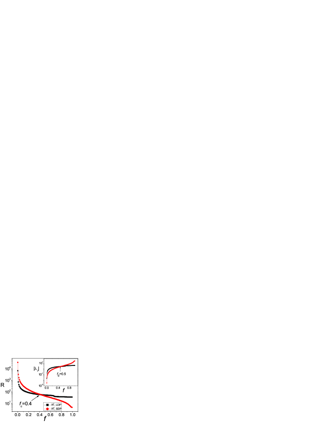
Figure 1: (Color online) With pinning strength $\eta=25$, the comparison of the performance between the LDP and SDP strategies in controlling a scale-free network. Inset: the variations of the largest non-zero eigenvalue as a function of the fraction of pinned nodes. Each data is averaged over $20$ network realizations.

Having specified the pinning model, we now compare the performance of the two pinning strategies, namely LDP and SDP, based on numerical simulations. Without loss of generality, we generate a complex network by the standard BA algorithm CN:REV , which consists of $N=1000$ nodes and has average degree $\left<k\right>=8$. The node degree of the generated network follows roughly a power-law distribution $p(k)\sim k^{-\gamma}$, with $\gamma=3$. The LDP and SDP strategies are implemented as follows. We first rearrange the nodes by a descending order of their degree, i.e. $k_{1}>k_{2}\ldots>k_{N}$. Then, in LDP the $n$ largest-degree nodes are pinned all together, i.e., nodes of index $1\leq m\leq n$ are pinned; while in SDP, the $n$ smallest-degree nodes are pinned i.e., nodes of index $N-n+2\leq m\leq N+1$ are pinned. The eigenratio of the two pinned networks are denoted by $R^{L}$ (LDP) and $R^{S}$ (SDP). The variations of $R^{L}$ and $R^{S}$ as a function of the fraction of pinned nodes, $f=n/N$, are plotted in Fig. 1. Interestingly, we find that, when the number of pinned nodes is large enough, $R^{S}$ is smaller than $R^{L}$, i.e., the SDP strategy has a higher performance than the LDP strategy. More specifically, there exists a critical fraction, $f_{c}\approx 0.4$, in the number of pinned nodes. When $f$ is small, as tacitly believed, the LDP strategy has the higher performance than the SDP strategy. However, as $f$ increases, the advantage of LDP over SDP is gradually narrowed and, at the critical value $f_{c}$, the two strategies give the same performance. After that, the SDP strategy will outperform the LDP strategy. Moreover, as $f$ increases from $f_{c}$, the advantage of SDP over LDP is gradually enlarged. The difference between the two strategies reaches its maximum at $f=1-1/N$, where only the small-degree (largest-degree) node is un-pinned in LDP (SDP). Of course, at the point $f=1$ the network is globally controlled, and the two strategies give the same performance again. (The switch of control performance is also observed in the variation of $\lambda_{2}$, which characterizes the system controllability for the situation of non-bounded MSF function HCLP:2009 .)

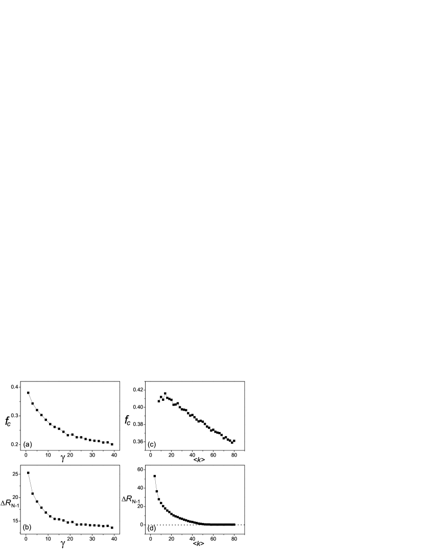
Figure 2: The other parameters are the same as in Fig. 1. By varying the degree exponent, the variations of (a) the critical fraction $f_{c}$ and (b) the performance difference between SDP and LDP at $n=N-1$. (b) and (c), the variations of $f_{c}$ and $\Delta R_{N-1}$ as a function of the network average degree. Each data is averaged over $20$ network realizations.

Is the above phenomenon general for complex networks? To answer this question, we have compared the performance of the two strategies on a variety of networks, including changing the degree exponent, the average degree, the network size and the pinning strength of the network model used in Fig. 1. In exploring the influence of the degree exponent $\gamma$, we have adopted the network model of Ref. DM:2002 , where $\gamma$ can be increased from $3$ to a large value by tuning a parameter. In doing this, the network topology is changing from heterogenous to homogeneous gradually. The variation of the critical fraction $f_{c}$ as a function of $\gamma$ is plotted in Fig. 2(a), where it is found that the value of $f_{c}$ is monotonically decreased. Meanwhile, with the increase of $\gamma$, the performance difference between the two strategies, $\Delta R=R^{L}-R^{S}$, is narrowed, e.g, the variation of $\Delta R$ at $n=N-1$ [Fig. 2(b)]. The narrowed difference in Fig. 2(b) seems to implies that, comparing to homogeneous networks, heterogeneous networks are more favorable for SDP. To check the influence of the average degree, we have increased the value of $\left<k\right>$ from 6 to 80. The variations of the critical fraction and the performance difference between the two strategies are plotted in Fig. 2(c) and (d), respectively. It is seen that, as $\left<k\right>$ increases, both $f_{c}$ and $\Delta R$ are decreased. Besides degree exponent and average degree, we have also checked the influence of the network size, and found that, as $N$ increases from 1000 to 5000, the values of $f_{c}$ and $\Delta R$ are decreased too (not shown). Noticing the fact that either the increase of $\left<k\right>$ or the decrease of $N$ leads to a homogeneous network structure, these additional simulations therefore confirm the finding of tuning $\gamma$, i.e., the SDP strategy for more favorable in controlling heterogeneous networks.

The existence of $f_{c}$ can be mathematically analyzed, based on the model of star networks. When not pinned, the star network has three distinct eigenvalues: $\lambda_{1}=0$, $\lambda_{N}=-N$, and $\lambda_{i}=-1$ for $i=2,\ldots,N-1$. When pinned, the eigenvalue spectrum will be modified, reflected as the decreases of $\lambda_{1}$, $\lambda_{N}$ and a few of other eigenvalues. Specifically, when $n$ nodes are pinned, in LDP the number of modified eigenvalues is $n+1$, while in SDP this number is $n+2$. Firstly, let us consider the case of $n=1$ and compare the performance of the two strategies. For LDP, only the central node is pinned, and the two modified eigenvalues, $\lambda^{L}_{1}$ and $\lambda^{L}_{N}$, are governed by equation

$$\lambda^{2}+(N+\eta)\lambda+\eta=0.$$ (2)

We thus have $\lambda^{L}_{1,N}=[-(N+\eta)\pm\sqrt{(N+\eta)^{2}-4\eta}]/2$. For SDP, the pinned node could be any of the $N-1$ peripheral nodes. The three modified eigenvalues, $\lambda^{S}_{1}$, $\lambda^{S}_{N-1}$ and $\lambda^{S}_{N}$, are governed by equation

$$-(\lambda^{2}+N\lambda+1)\eta=(\lambda+N)(\lambda+1)\lambda.$$ (3)

By Cardan formula, we have $\lambda^{S}_{1}=-(N+1+\eta+\omega_{1}p^{1/3}+\omega_{2}q^{1/3})/3$ and $\lambda^{S}_{N}=-(N+1+\eta+p^{1/3}+q^{1/3})/3$, where $p=(a+\sqrt{a^{2}-4b^{3}})/2$, $q=(a-\sqrt{a^{2}-4b^{3}})/2$, $a=2(N+1+\eta)^{3}-9N(N+1+\eta)(1+\eta)+27\eta$, $b=(N+1+\eta)^{2}-3N(1+\eta)$, and $\omega_{1,2}=-0.5\pm 0.5\sqrt{3}i$. Previous studies have shown that, to control the dynamics of a complex network successfully, the pinning strength should be sufficiently large, i.e., $\eta>>1$ XFW:2002 ; XL:2004 ; TC:2007 . Under this condition, the above eigenvalues are approximated as $\lambda^{L}_{1}\approx-1$, $\lambda^{L}_{N}\approx-(\eta+N)$, $\lambda^{S}_{1}\approx-1/N$, $\lambda^{S}_{N}\approx-(\eta+1)$. Apparently,

$$R^{S}=\lambda^{S}_{N}/\lambda^{S}_{1}>R^{L}=\lambda^{L}_{N}/\lambda^{L}_{1},$$ (4)

i.e., LDP has the higher performance than SDP when 1 node is pinned.

We next compare the performance of the two strategies for the situation of $n=N-1$, i.e. at the end of the comparison. For LDP, this means that except one peripheral node, all other nodes on the network are pinned. In this case, the eigenvalues $\lambda^{L}_{N-1}$ and $\lambda^{L}_{N-1}$ are governed by equation

$$-[(N+2\lambda)\eta+\eta^{2}](\lambda+1)+\eta=(\lambda+N)(\lambda+1)\lambda.$$ (5)

While for SDP, only the central node is un-pinned. In this case, the eigenvalues $\lambda^{S}_{N-1}$ and $\lambda^{S}_{N-1}$ are governed by equation

$$\lambda^{2}+(N+\eta)\lambda+N\eta=0.$$ (6)

Under the condition $\eta>>1$, these eigenvalues are approximated as $\lambda^{L}_{1}\approx-1$, $\lambda^{L}_{N}\approx-(\eta+1)$, $\lambda^{S}_{1}\approx-N$, $\lambda^{S}_{N}\approx-(\eta+1)$. So, when $N-1$ nodes are pinned, we have

$$R^{S}=\lambda^{S}_{N}/\lambda^{S}_{1}<R^{L}=\lambda^{L}_{N}/\lambda^{L}_{1},$$ (7)

i.e., SDP has the higher performance than LDP. Since the situations $n=1$ and $n=N-1$ stand as the two ends of the comparison [Fig. 1], Eqs. [4] and [7] thus guarantee the existence of at least one crossing in the performance curves.

The above phenomenon of performance switching can be physically explained as follows. Still take the star-network as the model. When only one node is pinned, by pinning the largest-degree node, the pinning signal can be efficiently propagated to the peripheral nodes, as the hub-node has the shortest average-node-distance. For this reason, LDP will have a higher performance than SDP (see Eq. [4]). However, this picture is changed when $N-1$ nodes are pinned. Under a strong pinning strength ($\eta>>1$), in LDP the $N-1$ pinned nodes have been well controlled to the target, and they will influence the un-pinned peripheral node via a coupling of strength $\varepsilon$; on the other hand, in SDP all the peripheral nodes have been controlled, and they influence the central node together via a joint coupling of strength $(N-1)\varepsilon$. Therefore in SDP the coupling between the pinned part (the peripheral nodes) and the un-pinned part is in fact amplified by $N-1$ times, therefore making SDP superior to LDP. Having understood this mechanism, we are able to predict that, as the size of the star network increases, the advantage that SDP over LDP will be enlarged. Actually, this point can be also drawn from Eq. [7], which implies that $\Delta R=R^{L}-R^{S}\propto N$. As the degree of heterogeneity of star networks can be characterized by the network size, this relation thus implies from another angle the superiority of SDP in controlling heterogeneous networks. It is worth noting that a similar phenomenon about the role of small-degree nodes has been also observed in network synchronization, where it is found that, to achieve global network synchronization, it is usually the smallest-degree nodes that are more important FMA:2006 .

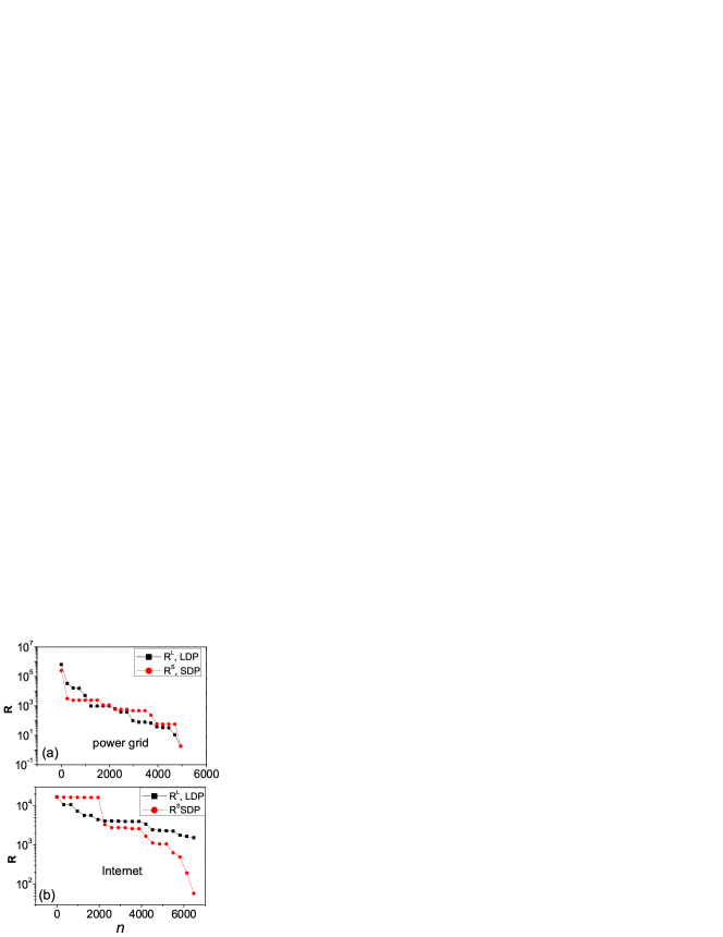
Figure 3: (Color online) Comparison of performance the two pinning strategies, LDP and SDP, for (a) the power-grid network of the western United States and (b) the Internet at the Autonomous level.

How about the realistic networks? The specific examples we have checked are the electrical power grid of the western United States USPOWER and the Internet at the autonomous level INTERNET . The power-grid network consists of $N=4941$ nodes and has average degree $\langle k\rangle\approx 2.67$. The variations of $R$ as a function of $n$ for both pinning strategies are plotted in Fig. 3(a). Interestingly, it is found that, different to the results of the ideal models [Fig. 1], the value of $R$ is decreased in a non-smooth fashion and the two curves are crossed at several places. We attribute this phenomenon to the inherent community structures in the power-grid network (a detail analysis on the non-smooth variation of $R$ will be presented elsewhere). The Internet we have employed consists of $N=6474$ nodes and having an average degree $\langle k\rangle\approx 3.88$. The variations of $R$ as a function of $n$ for both pinning strategies are plotted in Fig. 3(b). Again, we find a non-smooth decrease of $R$. For the Internet network, we find only one crossing between the two curves, which is located at about $n=2236$.

The finding that heterogenous networks can be better controlled by pinning the small-degree nodes might have some potential applications, say, for example, in synchronizing sensor networks or controlling the consensus of multi-agent systems. In a sensor network, due to terrain complexity the sensors are distributed in a non-uniform fashion: most of the sensors have very few neighbors, but a few sensors could have many neighbors SENSOR . That is, the sensor network has a heterogenous degree distribution. To synchronize the timers of the sensors, a general approach is to assemble a fraction of the sensors with a signal receiver, which receives signal from the satellite and reset the timer of the sensors accordingly. For those sensors without the receiver, their timers are updated by their neighbors. Here an important question is that, for the given number of sensors having signal receiver, how to place them properly in order of a higher performance for timer synchronization? The study of the current paper suggests that, if the number of receiver-assembled sensors are large enough, it may be better to place them in the areas of sparse sensors. Another application could be the control of consensus in multi-agent systems LS:2009 . To make the mobile agents move in a synchronous fashion, in engineering one practical approach is to introduce some “leading” agents into the system. Different to the normal agents, these leading agents have a predefined motion, but they will influence the motion of the normal agents via couplings (behave like the pinning controller). Our study suggests that, to control the multi-agent system more efficiently, we may choose to put the “leading” agents into the small swarms, instead of the tacitly believed large swarms. (From the network point of view, large and small swarms could be regarded as possessing large and small degree, respectively.)

In summary, we have compared the performance of two opposite pinning strategies in controlling complex networks. It is found that, when a significant fraction of the network nodes are pinned, the pinning of the small-degree nodes could have a higher performance than the large-degree ones. We have explained this phenomenon by a model of simplified network, and discussed the dependence of this phenomenon to the network parameters in detail. These findings, hopefully, will provide a new angle to the pinning control of complex networks, and apply to practical situations.

This work was supported by National Natural Science Foundation of China under Grant No. 10805038 and by Chinese Universities Scientific Fund.

References

- (1) G. Hu and Z. Qu, Phys. Rev. Lett. 72, 68 (1994).
- (2) G. Hu, Z. Qu, and K.F. He, Int. J. Bifurcation and Chaos 5, 901 (1995).
- (3) P.Y. Wang, P. Xie, J.H. Dai, and H.J. Zhang, Phys. Rev. Lett. 80, 4669 (1998).
- (4) G.N. Tang, K.F. He, and G. Hu, Phys. Rev. E 73, 056303 (2006).
- (5) M. D. Shrimali, Chaos 19, 033105 (2009).
- (6) R.O. Grigoriev, M.C. Cross, and H.G. Schuster, Phys. Rev. Lett. 79, 2795 (1997).
- (7) J.H. Xiao, G. Hu, J.Z. Yang, and J.H. Gao, Phys. Rev. Lett. 81, 5552 (1998).
- (8) S. Guan, G.W. Wei, and C.-H. Lai, Phys. Rev. E 69, 066214 (2004).
- (9) G. Tang and G. Hu, Phys. Rev. E 73, 056307 (2006).
- (10) G. Hu, J.H. Xiao, J.Z. Yang, F.G. Xie, and Z. Qu, Phys. Rev. E 56, 2738 (1997).
- (11) X.F. Wang and G. Chen, Physica A 310, 521 (2002).
- (12) X. Li, X.F. Wang, and G. Chen, IEEE, Trans. Circuits Syst. 51, 2074 (2004).
- (13) T. Chen, X. Liu, and W. Lu, IEEE, Trans. Circuits Sys. 54, 1317 (2007).
- (14) F. Sorrentino, CHAOS 17, 033101 (2007).
- (15) Y. Zou and G. Chen, Europhys. Lett. 84, 58005 (2008).
- (16) J. Zhao, J. Lu, and Q. Zhang, IEEE, Trans. Circuits Sys. 56, 514 (2009).
- (17) R. Albert and A.-L. Barabási, Rev. Mod. Phys. 74, 47 (2002).
- (18) A. Arenas, A. Diaz-Guilera, J. Kurths, Y. Moreno, and C. Zhou, Phys. Rep. 469, 93 (2008).
- (19) M. Zhan, J. Gao, Y. Wu, and J.H. Xiao, Phys. Rev. E 76, 036203 (2007).
- (20) L.M. Pecora and T.L. Carroll, Phys. Rev. Lett. 80, 2109 (1998).
- (21) G. Hu, J.Z. Yang, and W. Liu, Phys. Rev. E 58, 4440 (1998).
- (22) L. Huang, Q. Chen, Y.-C. Lai, and L.M. Pecora, Phys. Rev. E 80, 036204 (2009).
- (23) S.N. Dorogovtsev and J.F.F. Mendes. Adv. Phys. 51, 1079 (2002).
- (24) F. M. Atay, T. Biyikoglu, and J. Jost, Physica D 224,35 (2006).
- (25) ftp://ftp.santafe.edu/pub/duncan/power_unweighted
- (26) http://moat.nlanr.net/AS/Data/ASconnlist.20000102.946809601
- (27) F. Sivrikaya and B. Yener, IEEE Network 18, 45 (2004).
- (28) L. Wang and Y.-X. Sun, J. Stat. Mech. 11, 11005 (2009).