The extreme luminosity states of Sagittarius A*

We discuss mm-wavelength radio, 2.2-11.8$\mu$m NIR and 2-10 keV X-ray light curves of the super massive black hole (SMBH) counterpart of Sagittarius A* (SgrA*) near its lowest and highest observed luminosity states. We investigate the structure and brightness of the central S-star cluster harboring the SMBH to obtain reliable flux density estimates of SgrA* during its low luminosity phases. We then discuss the physical processes responsible for the brightest flare as well as the faintest flare or quiescent emission in the NIR and X-ray domain. To investigate the low state of SgrA* we use three independent methods to remove or strongly suppress the flux density contributions of stars in the central 2” diameter region around SgrA*. The three methods are: a) low-pass filtering the image; b) iterative identification and removal of individual stars; c) automatic point spread function (PSF) subtraction. For the lowest observed flux density state all 3 image reduction methods result in the detection of faint extended emission with a diameter of 0.5” - 1.0” and centered on the position of SgrA*. We analyzed two datasets that cover the lowest luminosity states of SgrA* we observed to date. In one case we detect a faint K-band (2.2$\mu$m) source of $\sim$4 mJy brightness (de-reddened with $A_{K}$=2.8) which we identify as SgrA* in its low state. In the other case no source brighter or equal to a de-reddened K-band flux density of $\sim$2 mJy was detected at that position. As physical emission mechanisms for SgrA* we discuss bremsstrahlung, thermal emission of a hypothetical optically thick disk, synchrotron and synchrotron self-Compton (SSC) emission, and in the case of a bright flare the associated radio response due to adiabatic expansion of the synchrotron radiation emitting source component. The luminosity during the low state can be interpreted as synchrotron emission from a continuous or even spotted accretion disk. For the high luminosity state SSC emission from THz peaked source components can fully account for the flux density variations observed in the NIR and X-ray domain. We conclude that at near-infrared wavelengths the SSC mechanism is responsible for all emission from the lowest to the brightest flare from SgrA*. For the bright flare event of 4 April 2007 that was covered from the radio to the X-ray domain, the SSC model combined with adiabatic expansion can explain the related peak luminosities and different widths of the flare profiles obtained in the NIR and X-ray regime as well as the non detection in the radio domain.

1 Introduction

Table 1: The brightest X-ray flares from SgrA*. For references see text.

label	date	Observatory	$\alpha=\Gamma-1$	X-ray flux	NIR L-band	11.8$\mu$m
				density	flux density	flux density
				($\mu$Jy)	(mJy)	(mJy)
$\alpha$	Oct. 26/27, 2000	Chandra	0.0$\pm$0.8	0.65$\pm$0.07	-	-
$\beta$	Oct. 3, 2002	XMM	1.2$\pm$0.3	2.7$\pm$0.4	-	-
$\gamma$	Apr. 4, 2007	XMM	1.3$\pm$0.3	1.7$\pm$0.3	20$\pm$2	$<$3$\sigma$=57

Table 2: Details on observing runs during which SgrA* was in a very low NIR luminosity state.

Telescope	Instrument	$\lambda$	UT and JD	UT and JD
Observing ID			Start Time	Stop Time
VLT UT 4	NACO	2.2 $\mu$m	2004 23 Sept. 23:20:45	2004 24 Sept. 01:45:11
			JD 2453272.47969	JD 2453272.57304
VLT UT 4	NACO	2.2 $\mu$m	2004 30 Aug. 23:49:36	2004 31 Aug. 01:28:19
			JD 2453248.48375	JD 2454466.50000

At the center of the Milky Way stellar motions and variable emission allow us to firmly associate Sagittarius A* (SgrA*) with a 4$\times$10⁶ M_⊙ super-massive black hole (Eckart & Genzel 1996, Genzel et al. 1997, 2000, Ghez et al. 1998, 2000, 2003, 2005a, 2008, Eckart et al. 2002, Schödel et al. 2002, 2003, 2009, Eisenhauer 2003, 2005, Gillessen et al. 2009).

Recent radio, near-infrared and X-ray observations have detected variable and polarized emission and give detailed insight into the physical emission mechanisms at work in SgrA*,which may include any or all of synchrotron, SSC, and bremsstrahlung emission (e.g. Baganoff et al. 2001, 2002, 2003, Eckart et al. 2003, 2004, 2006ab, 2008ab, 2009, Porquet et al. 2003, 2008, Goldwurm et al. 2003, Genzel et al. 2003, Ghez et al. 2004ab, Eisenhauer et al. 2005, Belanger et al. 2006, Hornstein et al. 2007, Yusef-Zadeh et al. 2006ab, 2007, 2008, 2009, Marrone et al. 2009, Dodds-Eden et al. 2009). Multi wavelength detections of the radio point source at sub-millimeter, X-ray, and infrared wavelengths have also been made, showing that the luminosity associated with SgrA* is on the order of 10^-9…-10 times below the Eddington luminosity L_Edd and many orders of magnitudes below that of SMBHs in active galactic nuclei (AGN) with comparable masses (of about 4$\times$10⁶M_⊙ ). The surprisingly low luminosity has motivated many theoretical and observational efforts to explain the processes that are at work in Sgr A*. For a recent summary of accretion models and variable accretion of stellar winds onto Sgr A* see Yuan (2006) and Cuadra & Nayakshin (2006, 2009).

Sgr A* is - in terms of Eddington luminosity - the faintest super-massive black hole known. However, due to its proximity it is bright enough to be studied in great detail. With the possible exception of the closest galaxies, no extragalactic super-massive black hole with a similar feeble Eddington rate would be observable. Motivated by the need to explain the variable luminosity of SgrA* we have analyzed data from it highest and lowest states. In order to separate the weak NIR emission of Sgr A* from the surrounding stars, the use of large telescopes and adaptive optics (AO) is required. Here we present the first attempt to do this with near-infrared data obtained with the VLT. Likewise, high resolution is needed in the X-ray regime to separate Sgr A* from the surrounding diffuse X-ray background.

The temporal correlation between the rapid variability of the near-infrared (NIR) and X-ray emission suggests that the emission showing 10^33-35 erg/s flares arises from a compact source within a few tens of Schwarzschild radii of the SMBH. For SgrA* we assume $R_{s}$=2$R_{g}$=2GM/c²$\sim$10¹⁰ $m$ for a $\sim$4$\times$10⁶M_⊙  black hole. Here $R_{s}$ is one Schwarzschild radius and $R_{g}$ the gravitational radius of the SMBH. One R_s then corresponds to an angular diameter of $\sim$8 $\mu$as at a distance to the Galactic center of $d=8\leavevmode\nobreak\ kpc$ (Reid 1993, Eisenhauer et al. 2003, Ghez et al. 2005ab). These observations can be explained in a model of an intrinsically faint accretion disk that is dominated by red-noise and temporarily harbors a bright orbiting spot possibly in conjunction with a short jet (Eckart et al. 2006b, Meyer et al. 2006ab, 2007). The phenomenon can best be studied through the brightest flares that allow us to derive high signal to noise light curves and multi wavelength observations throughout the electromagnetic spectrum.

In its lowest luminosity states SgrA* is difficult to detect though due to the presence of a strong diffuse background at X-ray wavelengths and the confusion with nearby stellar sources in the near-infrared. Here we discuss the relative importance of the bremsstrahlung and SSC process for the low state of SgrA* and investigate if the brightest flares of SgrA* can be explained via a SSC model involving up-scattered sub-millimeter photons from compact source components. In Sects. 2 and 3 we describe the observations, the data reduction and the algorithms we used to extract SgrA* in its low state from the background emission of the dense cluster of high velocity stars at angular separations of less than about 1” from the position of SgrA*. Below we will refer to this association of stars as the ’S-star cluster’. In Sect. 4 we present and discuss results. We start by summarizing the results of our deep Ks imaging in subsections 4.1 and 4.2. In the following subsections we then discuss various emission mechanisms for the low and high luminosity states of SgrA*. We show that the SSC process can successfully discribe both the low and high luminosity states and that - in particular for the high states - no extra mechanisms need to be involved (discussion in e.g. Dodds-Eden et al. 2009, Eckart et al. 2009). A brief summary and conclusions are presented in Sect. 5.

Throughout the paper we quote de-reddened infrared flux densities using a Ks-band (2.2$\mu$m) extinction correction of $A_{Ks}=2.8$ (Scoville et al. 2003, Schödel et al. 2007, Schödel et al. 2010 in prep., Buchholz, Schoedel, Eckart 2009). In Sect. 4.1 we use $\Gamma$ and $\gamma$ to describe the projected and three dimensional structure of the central stellar cluster respectively. In Table 1 and starting with subsection 4.4 we use $\Gamma$ and $\gamma$ as the bulk boosting factor and the relativistic electron Lorentz factor.

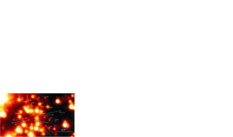
Figure 1: Identification of individual sources that were used for the iterative subtraction of the Ks-band datasets (Table 2). Here we show the image derived from the 23 September 2004 data. The nomenclature was taken from the deconvolved H-band image given in Fig.1 by Gillessen et al. (2006). Sources that are not contained in there have labels starting with ’N’. Relative positions and flux densities of the labeled sources are given in Table 3.

Table 3: Sources used for iterative source subtraction for the 23 September 2004 data.

name	other	$\Delta$$\alpha$	$\Delta$$\delta$	$R$	flux	Ks	K’-0.2	$\Delta$mag
	name	arcsec	acrsec	arcsec	mJy
S62		0.01	-0.02	0.03	1.52	17.0
S17	S0-17	0.02	-0.09	0.09	8.06	15.2	15.5	-0.3
S38?		-0.08	0.05	0.10	1.27	17.2
S55		0.07	-0.09	0.11	0.71	17.9
S40		0.12	0.00	0.12	1.88	16.8
S2	S0-2	0.02	0.13	0.13	22.00	14.1	13.9	0.2
S13?	S0-8	-0.11	0.09	0.14	7.04	15.4	?
S19		0.06	-0.15	0.16	1.79	16.9
S14		0.16	0.12	0.20	7.41	15.3
S18	S0-38	-0.20	-0.06	0.21	2.19	16.7	?
S44		-0.08	-0.23	0.24	1.13	17.4
S20		0.21	0.12	0.24	8.80	15.1
S39		-0.10	0.23	0.25	1.37	17.2
S1	S0-1	0.00	-0.25	0.25	14.00	14.6	14.5	0.1
S63		0.24	-0.13	0.28	1.20	17.3
S4	S0-3	0.29	0.12	0.31	14.02	14.6	14.3	0.3
S22		0.17	-0.27	0.32	2.39	16.6
S12		-0.06	0.31	0.32	8.04	15.2
S23		0.32	-0.08	0.33	1.01	17.5
S52		0.19	0.27	0.33	0.98	17.5
NS2		0.18	0.32	0.36	1.06	17.4
S21		-0.33	-0.14	0.36	2.03	16.7
S36		0.27	0.25	0.36	3.66	16.1
S60/59	S0-12	-0.29	0.24	0.37	6.70	15.4	14.2	1.2
S41		-0.23	-0.31	0.38	1.10	17.4
S10	S0-6	0.04	-0.38	0.38	21.99	14.1	14.0	0.1
S5		0.34	0.19	0.39	9.47	15.1
S42		-0.17	-0.37	0.40	1.62	17.0
S9	S0-5	0.18	-0.36	0.40	12.66	14.7	14.9	-0.2
S57		0.42	-0.14	0.44	0.89	17.6
S25	S0-18	-0.11	-0.43	0.44	10.71	14.9	?
S47		0.38	0.23	0.45	2.73	16.4
S28		-0.01	0.46	0.46	1.56	17.0
S6		0.47	0.09	0.48	8.02	15.2
S8	S0-4	0.39	-0.28	0.48	17.72	14.4	14.3	0.1
S32		0.33	-0.36	0.49	2.85	16.4
NS1		0.27	0.42	0.50	1.81	16.9
S37		0.33	0.38	0.50	2.74	16.4
S7	S0-11	0.51	-0.05	0.51	10.38	15.0	15.1	-0.1
S43		-0.51	-0.15	0.53	1.30	17.2
S29		-0.21	0.49	0.54	2.33	16.6
S27	S0-27	0.14	0.53	0.55	7.34	15.3	15.5	-0.2
S49		0.56	0.04	0.56	1.60	17.0
S45		0.19	-0.52	0.56	7.59	15.3
S24	S0-28	-0.16	-0.54	0.56	6.26	15.5	15.6	-0.1
S53		0.29	0.49	0.57	1.30	17.2
S34		0.32	-0.47	0.57	8.55	15.2
S11	S0-9	0.17	-0.58	0.60	23.79	14.1	14.2	-0.1
S46		0.24	-0.56	0.61	6.92	15.4
S48		0.44	0.45	0.63	3.21	16.2
S35	S0-13	0.54	-0.43	0.69	45.90	13.3	13.3	0.0

2 Observations and data reduction

Near-infrared (NIR) observations of the Galactic center (GC) were carried out with the NIR camera CONICA and the adaptive optics (AO) module NAOS (briefly “NACO”) at the ESO VLT unit telescope 4 (YEPUN) on Paranal, Chile. The data were taken on the night of 30 August and 23 September, 2004. The dataset taken on 23 September 2004 turned out to be the best available set in which SgrA* is in a quiet state. During the 30 August observations some weak activity at 2.2$\mu$m could be detected, making this dataset well-suited to determine the position of SgrA* with respect to neighboring stars. The combination of both datasets is ideally suited to obtain a flux density estimate or limit of SgrA* in its quiet state.

For all observations the infrared wavefront sensor of NAOS was used to lock the AO loop on the NIR bright (Ks-band magnitude $\sim$6.5) supergiant IRS 7, located about $5.6^{\prime\prime}$ north of Sgr A*. The pixel scale was 13.27 mas.

The atmospheric conditions (and consequently the AO correction) were stable during the observations. The seeing at the telescope measured in the optical was $\sim$0.6”. We used an integration time of DIT=2 seconds and a number of integrated images of NDIT=15. Details on start and stop times are listed in Table 2.

All observations in the Ks-band (2.2 $\mu$m) were dithered to cover a larger area of the GC by mosaic imaging. The sky background for the Ks-band observations was extracted from the median of stacks of dithered exposures of a dark cloud – a region practically empty of stars – about 400” north and 713” west of the target. All exposures were sky-subtracted, flat-fielded, and corrected for dead or bad pixels. The images were shifted and stacked in a cube with a mean average to get a mosaic image of the GC. All of these steps were performed with the DPUSER software for astronomical image analysis (T. Ott, MPE; see also Eckart & Duhoux 1990). Subsequently, PSFs were extracted from these images with StarFinder (Diolaiti et al. 2000) both for deconvolution with the Lucy-Richardson (LR Lucy 1974) algorithm and for PSF subtraction.

The flux densities of the sources were measured by aperture photometry with circular apertures of 40 mas radius and corrected for extinction, using $A_{K}=2.8$ (Scoville et al. 2003, Schödel et al. 2007, Schödel et al. 2010 in prep., Buchholz, Schoedel, Eckart 2009). Possible uncertainties in the extinction by a few tenths of a magnitude alter the infrared flux densities of SgrA* by a few 10%. These variations are easily compensated for by insignificant variations in the spectral indices or the boosting which do not influence the general results obtained in this paper.

The flux density calibration was carried out with the known Ks-band flux densities of IRS16C, IRS16NE, and IRS21 by Blum, Sellgren & Depoy (1996). Subsequently the relative photometry for Sgr A* was done using 10 sources within 1$\aas@@fstack{\prime\prime}$6 of Sgr A* as secondary calibrators (S67, S92, S35, S8, S76, S1, S2, S87, S65, S30; Gillessen et al. 2006). This results in a Ks-band flux density of the high velocity star S2 of 22$\pm$1 mJy, which compares well with the magnitude and flux for S2 quoted by Ghez et al. (2005b) and Genzel et al. (2003). The measurement uncertainties for Sgr A* were obtained on the nearby reference star S2. The background flux in the immediate vicinity of Sgr A* was obtained by averaging the measurements at six random locations in a field located about 0$\aas@@fstack{\prime\prime}$6 west of Sgr A* that is free of obvious stellar sources. A Ks-band image of the central 4.3”$\times$2.5” is shown in Fig. 1. This field is at the center of the stellar cluster of which we show a 15”$\times$15” overview in Fig. 2a). The source positions and relative astrometry was established via StarFinder. The positions in Table 3 are given relative to the position of SgrA* as determined from the 23 September 2004 data. We list the name following the nomenclature used by Gillessen et al. (2009) and in the second column the name used by Do et al. (2009b). Sources labeled with $N$ had not been identified before. Identifications with question marks are tentative and suffer most likely from the proper motion of faint sources between the present date and the date used for identification by Gillessen et al. (2009). Then we list in Table 3 the sky projected relative offsets $\Delta$$\alpha$, $\Delta$$\delta$ and radial distance $R$ from SgrA* in arcseconds. The uncertainties in the offsets are better than a third of a pixel i.e. 0.004” We then list in Table 3 the observed Ks magnitude derived in this paper and the observed K’ magnitude listed by Do et al. (2009b) corrected by an offset value of -0.2 magnitudes. The scatter between both values after correction for this offset is 0.2 magnitudes, so that the offset corresponds to 1$\sigma$ in magnitudes (20% in flux) and is well within the expected calibration uncertainties for faint stars in the crowded field. The difference between both mangitude values is listed in the last column. For sources S0-8, S0-18 and S0-38 no magnitudes are given by Do et al. (2009b). The large magnitude difference in the case of S0-12 is most likely due to the blend of S59 and S60. The two NIR filters $K_{s}$ and K’ (Do et al. 2009b) are very similar with Ks(NACO): $\lambda_{center}$=2.18$\mu$m and width $\Delta$$\lambda$=0.35$\mu$m and K‘(NIRC): $\lambda_{center}$=2.124$\mu$m and width $\Delta$$\lambda$=0.351$\mu$m. No transformation between magnitudes derived with these filters was applied. The 0.2 mag scatter relates to stars of different brightnesses at different epochs between which they are moving at different locations in the cluster with respect to different local backgrounds. The relative flux density uncertainty for the star S2 - which we use as an estimate for SgrA* - is determined within a single epoch at fixed position.

3 Subtracting stars

To investigate the low luminosity state of SgrA* we use three independent methods to remove or strongly suppress the flux density contributions of stars in the central 2” diameter region around SgrA*. All three methods give comparable results and allow us to clearly determine the stellar light background at the center of the Milky Way against which SgrA* has to be detected.

We assume that the PSF as determined from stars in the central few arcseconds of the image is uniform across the central S-star cluster. Investigations of larger images (e.g. Buchholz et al. 2009) show that on scales of a few arcesconds this is a reasonable assumption and that PSF variations have to be taken into account only for fields $\geq$10”. Whether the residual extended emission we find close to SgrA* is due to rsiduals from the subtracting algorithms or associated with additional stellar emission from the S-star cluster is discussed in Sect. 4.1.

3.1 Linear extraction of extended flux density

With the point spread function $P$ and the object distribution $O$ we can write the formation of an image $I$ as

$$I=O*P=(\Delta+E)*P=\Delta*P+E*P\leavevmode\nobreak\ .$$ (1)

Here the symbol $*$ denotes the convolution operator. The variable $\Delta$ denotes the distribution of stellar sources and $E$ the distribution of extended emission. Both types of sources are assumed to be ideally unresolved or resolved with respect to the point spread function. To produce a high-pass filtered image we can calculate a smooth-subtracted image $\Sigma$ as

$$\Sigma=I*G-I=(\Delta+E)*P*G-(\Delta+E)*P\leavevmode\nobreak\ .$$ (2)

Here we use a narrow Gaussian $G$ normalized to an integral power of unity. This can be rewritten as

$$\Sigma=\Delta*(P*G-P)+(E*P*G-E*P)\leavevmode\nobreak\ .$$ (3)

Since the width of the extended emission is expected to be much larger than the full width at half maximum of the PSF, and in particular since the Gaussian $G$ is narrow with respect to $P$, we can infer that $E*P*G\sim E*P$. Then the differential point spread function $P*G-P$ is the PSF of the high-pass filtered differential image

$$\Sigma\sim\Delta*(P*G-P)\leavevmode\nobreak\ .$$ (4)

Since $\Sigma$ is fully dominated by the contribution of the distribution of unresolved stellar sources, this distribution $\Delta$ can be retrieved via a linear deconvolution of the differential image with the differential PSF

$$\Delta\sim\Sigma\leavevmode\nobreak\ \%\leavevmode\nobreak\ (P*G-P)\leavevmode\nobreak\ .$$ (5)

Here the symbol $\%$ denotes the deconvolution operation. Consequently the distribution of extended flux (i.e. a low-passed filtered version of the image) $E*P$ can now be isolated via

$$E*P=I-\Delta*P$$ (6)

or

$$I-\Sigma*P\leavevmode\nobreak\ \%\leavevmode\nobreak\ (P*G-P)=\Delta*P+E*P-\Delta*P=E*P\leavevmode\nobreak\ .$$ (7)

The advantage of this new method is that it is independent of input models, i.e. it does not depend on the identification of individual stars or on assumptions on the existence or properties of a diffuse background flux density distribution. Also the method only uses linear operations, i.e. image subtraction and linear convolution and deconvolution (Fourier multiplications and divisions). Therefore it is not dependent on the flux density of sources and numbers of iterations, as is the case for many non-linear algorithms (e.g. the Lucy-Richardson or maximum entropy algorithm). In order to demonstrate the validity of the approach we show the results we obtained on the central 15”$\times$ 15” of the 23 September data in Fig. 2. For all the prominent extended Ks-band sources (Fig. 2) the extended Ks-band emission can be retrieved and its structure compares very well to the previously published results (e.g. Ott, Eckart & Genzel 1999, Tanner et al. 2002, 2005). (A comparison of different deconvolution algorithms used in the crowded Galactic center field is given in Ott, Eckart & Genzel 1999.) At a dynamic range of about 100:1 we show in Fig. 2b) a low-pass filtered version of the Ks-band image that was obtained by following the algorithm outlined above. The prominent sources have been labeled with their names. In Figs. 2c), d) and e) we show the extended flux density distribution of the following sources: IRS 1W, IRS 21, IRS 10W. These bow-shock structures are shown at the angular resolution of about 0.1” as delivered by the AO system. They compare very well with the source structures published by Tanner et al. 2005. Here the algorithm detects very bright sources like IRS 7 also as an extended object since the star is overexposed and not well described by the used PSF. In Fig. 3 we show results of the algorithm on the central 2”$\times$ 2”. In addition to residuals of the filter process around the position of bright stars, we see an increased flux density level within the dashed 0.5” diameter circle centered on the position of SgrA*. The disadvantage of this algorithm is that any point-like emission from SgrA* is also strongly suppressed. The residuals (ringing) still evident around the bright stars are a consequence of the choice of the apodization filter that needs to be defined in the case of linear deconvolution. This filter is used to suppress the usual high spatial frequency noise that arises due to small number division problems. We used a cosine-bell shaped filter that preserves the high angular resolution but results in some residual ringing. However, the result on the background emission is not strongly influenced by this, since the bright stars are sufficiently far away from the central position. The comparison to the results of the other two algorithms used to remove the contributions of stars near SgrA* shows that the result is also little affected by the much fainter stars close to SgrA*. Their contribution has been efficiently suppressed by the algorithm.

3.2 Iterative PSF subtraction

The iterative PSF subtraction was carried out within the central 2” to 3” around the position of SgrA*. This was performed by resizing, shifting and scaling the PSF to the position and the value of each star and then subtract it. The sources used for this process are listed in Table 3 and are shown in Fig. 1. A total number of 51 stars were subtracted so that the resulting background was as smooth as possible. In Fig. 4 we show the resulting subtracted image of the area of interest around SgrA*. All stars brighter than about 17.5^m (see KLF in Fig. 6) have been subtracted with a scaled version of the PSF. The thin lines in Figs. 4a) and b) are used to triangulate the position of SgrA*. Fig. 4a) shows the image obtained from a section of the 30 August dataset with SgrA* flaring. Compared to S2 with $\sim$22 mJy SgrA* has a brightness of about 4 mJy. Fig. 4b) shows the image obtained from a section of the 23 September dataset with SgrA* in a quiescent phase. Here SgrA* is clearly not detected and is fainter than about 2 mJy (de-reddened).

Figure 4 also reveals the presence of faint residual extended emission - centered on the position of SgrA*. This residual emission is most likely from the central S-star cluster of high velocity stars. We determined the position of SgrA* from the data with SgrA* in a flare state taken on 30 August, 2004. Taking an upper limit of the observed two dimensional projected stellar velocity dispersion of $\sim$1000 km/s and the fact that for the Galactic center proper motion of 1 mas/yr corresponds to about 39 km/s, the relative positional uncertainty for stars observed between both epochs is expected to be well below 2 mas. Thin lines in Figs. 4a) and b) are used to triangulate the position of SgrA*. Figure 4 shows that for the dataset taken on 23 September 2004 no NIR counterpart of SgrA* was detected. For 30 August 2004 we find a NIR counterpart of SgrA* with a dereddened flux density of about 4 mJy with a 3$\sigma$ uncertainty of about 2 mJy. Estimates of the flux density limits and uncertainties are given in Sect. 4.2.

3.3 Automatic PSF subtraction

We also analyzed the images with the StarFinder (Diolaiti et al. 2000) program package. It not only provides accurate point source photometry but also a reliable estimation of the diffuse background emission. With a point spread function (PSF) extracted from bright stars near the guide star (in this case IRS 7), we performed photometry and astrometry on the deconvolved image via PSF fitting with the StarFinder package. The resulting diffuse background emission is shown in Fig. 5. In addition to some residual emission from unresolved stars this method also reveals extended emission centered on the position of SrgA* within the dashed 0.5” diameter circle centered on the position of SgrA*. This finding agrees with the low-pass filtered image in Fig. 3.

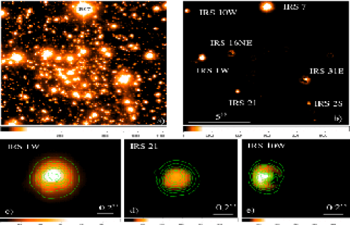
Figure 2: The Ks-band image of the Galactic center region (a) taken on 23 September 2004. The central 15”$\times$15” image was taken with the adaptive optics system NACO at the ESO VLT and the results of the low-pass filter algorithm. (b,c,d,e). The contour lines are separated by 8% of the peak brightness of IRS10W.

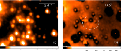
Figure 3: The inner 2”$\times$2” of the central stellar cluster (23 September 2004). The position of SgrA* is at the center of the images a) and b). In panel a) we show the corresponding image section taken out of the Ks-band image in Fig. 2 a). In panel b) we show the corresponding image section taken out of the low-pass filtered version in Fig. 2 b).

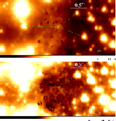
Figure 4: Results of the iterative star subtraction obtained for the 30 August (a) 23 September data (b) as described in Sect. 3.2.

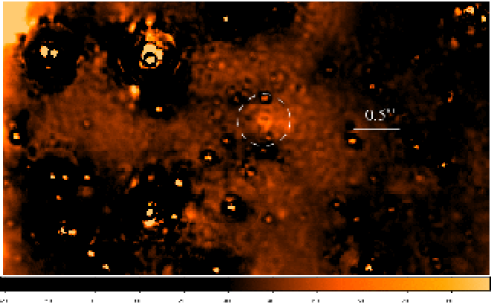
Figure 5: Result of the automatic PSF subtraction obtained for the 23 September 2004 data.

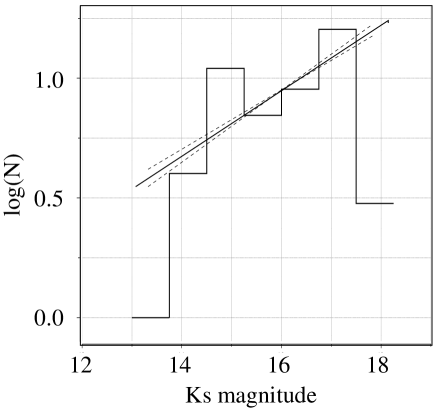
Figure 6: KLF histogram of the stars detected in the central field derived from the 23 September 2004 data. The straight full and dashed lines indicate the KLF slope of 0.21$\pm$0.02 found for radii of less than 6” by Buchholz et al. (2009).

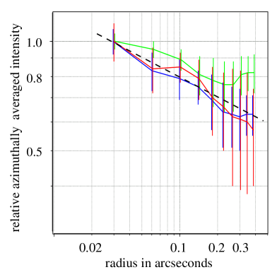
Figure 7: Azimuthal average of the diffuse background emission as derived from the three different methods applied: low pass filtering (red), manual PSF subtraction (green), and automatic PSF subtraction (blue). The curves (mean flux and 1$\sigma$ uncertainty per pixel) have been calculated in anuli of 39.8 mas (3 pixels) width and normalized to the value at 30 mas radius corresponding to one resolution element at 2.2$\mu$m. The black dashed line marks a profile with an exponential decrease of 0.2.

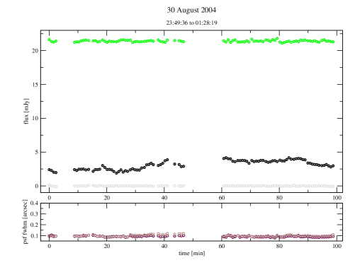
Figure 8: The 30 August 2004 light curve of the flux density measured in a 40 mas radius circular aperture centered on the position of SgrA* (black). We show the light curve of the reference star S2 in green. The bottom panel shows the FWHM seeing in arcseconds measured on the PSF extracted for the field. The grey points show the background counts near SgrA*. The width of the error bars is close to the size of the data points.

Figure 9: The same as Fig.8 but for 23 September 2004.

4 Results and discussion

First we analyze the properties of the central cluster of high velocity stars and compare them to the results of published investigations. We can then confidently derive the flux density limits on SgrA* and show that contributions to the lowest luminosity states from bremsstrahlung are unlikely. We then discuss the extreme luminosity states of SgrA* in the framework of a synchrotron self-Compton mechanism.

4.1 Imaging the S-star cluster and the detection of SgrA* in its low luminosity state

The detected number of 51 stars within a radial distance of about 0.5” from SgrA* results in a surface number density of 68$\pm$8 arcsec^-2, taking the square-root as the uncertainty of that value. This result agrees with the central number density of 60$\pm$10 arcsec^-2 given by Do et al. (2009b) in their Figs. 9 and 10.

Figure 6 shows the KLF histogram (K-band luminosity function) that can be derived for the stars detected in the central field. The binning of 0.75 magnitudes allows for a sufficient number of bins to clearly detect the linear slope in the double logarithmic plot and to have a sufficiently large number of sources per bin (about 10) at the same time. With d log(N)/d log(Ks)=0.3$\pm$0.1 the data compare well with the KLF slope of 0.21$\pm$0.02 found for the inner field ($R<6^{\prime\prime}$) by Buchholz et al. (2009).

Within the central 0.5 arcsecond radius region around SgrA* and in the magnitude interval ranging from Ks=16.75 to 17.50 no significant deviation from a straight powerlaw line can be detected - implying that the completeness is high and probably comparable to the $\sim$70% value derived for mag_K=17 by Schödel et al. (2007). In the interval ranging from Ks=17.50 to 18.25 the stellar counts drop quickly to about 20% of the value expected from the straight powerlaw line.

All three methods we used to correct for the flux density contribution of the stars in the central 2” reveal faint extended emission around SgrA* (see Figs. 3b, Fig. 4b and Fig. 5). For the iterative and automatic PSF subtraction the PSFs were extracted with a radius of 1”, which is about twice the FWHM of the S-star cluster. In case of a PSF misplacement a significant flux density contribution to the central position can only come from the about five stars that are located within one FWHM of SgrA*. They have a median brightness of about 2 mJy. To explain all of the $\sim$2 mJy at the center by this effect, each star would have to provide about 0.4 mJy or 20% of its flux density. This can only be realized by a systematic positional shift of these stars towards the center by about 1 pixel$\sim$13 mas each. Still, the positional accuracy which is typically reached is on the order of a few tenths of a pixel. Larger displacements result in a clearly identifiable characteristic plus/minus pattern in the residual flux distribution along the shift direction. However, allowing for a maximum positional uncertainty of 1 pixel and approximating the independent shifts of five stars by five shifts of a single star that follows a random walk pattern, the expected effective displacement is 1/$\sqrt{5}$ pixels for a single shift of each star. It will result in a 5% peak flux contribution of each of the 5 stars - assuming that the displacements are systematically towards the center, i.e. a total maximum contribution of 0.4 mJy. This implies that about one 20%-30% of the flux density detected at the center may be explained by a positional misplacement of the neighboring stars. Therefore we assume that the bulk (more than 2/3) of this extended emission toward the center can be associated with the $\sim$0.5”-1” diameter S-star cluster around SgrA* and is due to faint stars at or beyond the completeness limit reached in the KLF.

The extended residual emission is not distributed azimuthally uniform about the position of SgrA*. This is not expected either. The shape of the residual emission will always be dominated by the randomly distributed few brightest stars that contribute to it. Also the light of the central stellar cluster is not distributed azimuthally uniform on any scale: On scales larger than 0.5 pc it is affected by dust absorption (e.g. extinction map by Buchholz et al. 2009), on scales less than 0.5 pc the bright members of the IRS16 cluster are predominantly located to the east, and during the past decade in the central arcsecond most of the brighter S-stars have been located to the south and east of SgrA*.

The diffuse background emission can be compared to the projected distribution of stars $\Sigma(R)$$\propto$$R^{-\Gamma}$, with $R$ being the projected radius. Independent of the applied method we find that the azimuthally averaged residual diffuse background emission centered at the position of SgrA* decreases very gently as a function of radius (Fig. 7). The ratio between the brightness measured within or at the edge of the central resolution element (R$\sim$0.03”) and at a projected radius of e.g. R=0.2” is 1.5$\pm$0.15, corresponding to $\Gamma_{diffuse}$=0.20$\pm$0.05. This is consistent with the distribution of number density counts of the stellar populations in the central arcseconds derived from imaging VLT and Keck data. Buchholz et al. (2009) and Do et al. (2009b) find a $\Gamma$$\sim$1.5$\pm$0.2 for the young stars, but a much flatter distribution for the late-type (old) stars with $\Gamma$$\sim$0.17$\pm$0.09 or even $\Gamma$$\sim$-0.12$\pm$0.09, respectively. For pure imaging Do et al. (2009b) quote $\Gamma_{inner}$=0.19$\pm$0.06 inside a radius of R=3”.

In case of a relaxed stellar cluster around a supermassive black hole, stellar dynamics predicts to observe a cusp, i.e. a density increase toward the black hole with $\Gamma$ = $\gamma-1$ = 0.5 to 0.75 (Bahcall & Wolf 1976, Murphy 1991; Lightman & Shapiro 1977; Alexander & Hopman 2009). Here $\gamma$ denotes the exponent of the three dimensional distribution which does not suffer from projection effects but is harder to deduce from observed data. Only in the case of very extreme stellar densities collisions can lead to a $\Gamma$ as low as 0.5. But the required high densities are not reached in the Galactic center.

The observed values of $\Gamma$ are significantly lower than what is predicted by theory. The principal reason is probably to be sought in the stellar population in the central arcseconds, which towards Sgr A* becomes increasingly dominated by young massive stars that are too young to be dynamically relaxed. The small value of the projected diffuse light exponent $\Gamma_{diffuse}$$\sim$$\Gamma_{inner}$ may therefore imply the absence of a pronounced, relaxed cusp of stars.

However, there may in fact exist a deficit of late-type stars near Sgr A* (see also Genzel et al. 2003, Fig. 7). It may well be that most of the spectroscopically identified late type stars at small projected distances are at larger three dimensional radii $r$ $R$ from SgrA*. In this case the observed $\Gamma_{diffuse}$$\sim$$\Gamma_{inner}$ will be a mixture between the much steeper $\Gamma$_early for early type stars and the lower value $\Gamma$_late for late type stars. A detailed discussion is given in Do et al. (2009b), Buchholz et al. (2009), Schödel et al. (2007), and Genzel et al. (2003).

The main result for the present analysis of faint luminosity states of SgrA* is that the observed flat background light and number density distribution described by the exponent $\Gamma_{diffuse}$$\sim$$\Gamma_{inner}$ as well as the high degree of completeness reached around Ks=17.5 allows us to clearly distinguish the emission of SgrA* against the stellar light background at the center of the Milky Way. This also shows that SgrA* is ideally suited to perform a case study to investigate this super-massive black hole in its lowest activity state.

4.2 Observing SgrA* at low luminosities

High angular resolution images in the near-infrared allow us to unambiguously attribute bright dereddened flux levels to SgrA* (e.g. Genzel et al. 2003, Eckart et al. 2004, Ghez et al. 2004ab, Hornstein et al. 2006, Do et al. 2009a). The identification of fainter emission from SgrA* becomes increasingly difficult, since one can expect confusion from the $\sim$1” diameter S-star cluster that is centered on the location of Sgr A*. Due to the high proper motions of the stars within the S-star cluster this confusion also changes on the time scales of months to years. From the location of SgrA* Do et al. (2009a) find observed $0.082\pm 0.017$ mJy ($K^{\prime}=17.2$) or dereddened $1.75\pm$0.36 mJy (assuming their value of $A_{K^{\prime}}=3.3$) as the the faintest observed $K^{\prime}$ flux density (see also Hornstein et al. 2002 and Eckart et al. 2006). Using $A_{K^{\prime}}=2.8$ this results in a flux density of $1.1\pm$0.2 mJy

For the low flux density state Do et al. (2009a) reported red colors and variability compared to stellar sources. For the very low luminosity levels they report with an average power law exponent of -0.17$\pm 0.32$ a bluer spectrum than that reported earlier by Hornstein et al. (2002) with a power law slope of $0.6\pm 0.2$. The contamination from nearby (predominantly blue) stars is estimated to contribute a maximum of about 35% of the flux to account for this difference in the spectral slope. Do et al. (2009a) conclude that even when the emission is faint a large fraction of the flux arising from the location of SgrA* is likely non-stellar and can be attributed to physical processes associated with the black hole.

Our data allow us to provide a new independent estimate on the flux density of SgrA* in some of its lowest states based on VLT data.

In a circular aperture of a diameter of 66 mas diameter (5 pixels or about one resolution element) we measure dereddened flux densities (using $A_{K}=2.8$) 1.5$\pm$0.4 mJy, 1.3$\pm$0.3 mJy, and 1.3$\pm$0.2 mJy for the low-pass filtering, iterative, and automatic PSF subtraction method, respectively.

The uncertainties have been derived from the flux density measurements in the central 5$\times$5 pixel aperture and the upper limits of the measurement uncertainties per pixel as plotted in Fig. 7. These upper limits are 0.33 mJy, 0.24 mJy and 0.17 mJy for the three methods, respectively. Based on these data we derived an upper limit on the formal uncertainties in any random 5$\times$5 pixel aperture in the central 0.6” diameter field of 0.066 mJy, 0.048 mJy and 0.034 mJy for the three methods, respectively. We adopted these values for the central aperture. In order to obtain a conservative estimate we added in each case these values five times, so that the final uncertainty amounts to six times the value expected for an aperture of this size - based on the radial averages. There is no clear detection of a source at that position. If the observed flux density limit is fully attributed to SgrA* this corresponds to a clear non-detection of any point source at that position with a flux density limit of 2.4 mJy for SgrA* (K_s$\sim$16.3; observed reddened magnitude). If all of it is stellar, the upper limit is defined by the uncertainty of the measurement and the limit for a flux density from a non-stellar source at the position of SgrA* is 0.9 mJy (3$\sigma$, de-reddened and K_s$\sim$17.3 as an observed reddened magnitude). While our data do not allow us to confirm the existance of a constant quiescent state, our flux density limit is consistent with the flux given by Do et al. (2009a). This flux density limit is also consistent with the light curves of SgrA* shown in Figs.8 and 9. They were obtained in a 40 mas radius aperture centered at the position of SgrA*. The light curves were taken without removing any stars from the sourroundings and the aperture size of only 40 mas was chosen to minimize the contamination from neighboring stars. The bottom parts of Figs.8 and 9 show the FWHM of the PSF extracted on a nearby star. These graphs show that the seeing and AO performance were very stable and similar during the measurements on both dates. Especially in the second half of the 30 August light curve in Fig.8 SgrA* was sufficiently bright to be detected, while it was in a low state during the entire time during which the 23 September light curve in Fig.9 was taken. Our flux density limit for the 23 September data is consistent with the completeness limit we reached in the central star counts (see Sect.  4.1).

Figure 10: Sketch of the SgrA* surroundings within a 10⁵ Schwarzschild radius. The SMBH encloses the central 1 R_s volume surrounded by an edge on seen disk with indicated spots. The circles are logarithmically scaled and labeled with their radii in units of R_s. During and after flares the spots expand to meet the accretion flow density of about 10⁷cm^-3 at an approximate radius of 1000 R_s. The edge of the 1.4” FWHM size Bondi sphere is located at a radius of about $\sim$8$\times$10⁴R_S for a 4$\times$10⁶ M_⊙ (Baganoff et al. 2001, 2003).

4.3 Bremsstrahlung emission from SgrA*

4.3.1 The quiescent state X-ray emission from SgrA*

Baganoff et al. (2001, 2003) reported an extended (R$>$10³ R_s) thermal bremsstrahlung source co-spatial with the position of the strongly variable point source at the location of SgrA* (see also Quataert 2003). The authors derive 1.4”$\pm$0.14” for the intrinsic FWHM size of the source. This corresponds to $\sim$8$\times$10⁴R_S for a 4$\times$10⁶ M_⊙ black hole. The scale of the extended structure centered on SgrA* is consistent with the expected Bondi accretion radius (1”- 2”; Bondi 1952) for matter accreting hydrodynamically onto the SMBH. For the bright flare emission of the X-ray point source bremsstrahlung is not a likely mechanism to produce the observed NIR flux density excursions (Genzel et al. 2003, Yuan et al. 2003, Quataert, 2002). In part motivated by the blue spectrum reported by Do et al. (2009a) - assuming that not all of the blue character is due to stellar contamination - we investigate here if the lowest NIR flux density values can be explained by a bremsstrahlung contribution from a hot disk.

Table 4: Source component parameters for SSC models of the brightest X-ray flares from SgrA*.

model	$\gamma_{1}$	$\gamma_{2}$	Smax,	$\alpha_{synch}$	R0	$\nu_{max}$	B	SMIR,	SNIR,	SNIR,	SNIR,	SX-ray,
			obs			obs		synch	synch	synch	SSC	SSC
label			[Jy]			[GHz]	[G]	[mJy]	[mJy]	[mJy]	[mJy]	[$\mu$Jy]
								@11.8$\mu$m	@3.8$\mu$m	@2.2$\mu$m	@2.2$\mu$m	@2-10 keV
$1\leavevmode\nobreak\ \sigma$ $\rightarrow$			$\pm$0.1	$\pm$0.1	$\pm$0.1	$\pm$250	$\pm$10	$\pm$1.0	$\pm$1.0	$\pm$1.0	$\pm$1.0	$\pm$20
A$\alpha$	360	2900	1.9	1.19	0.3	1850	18	59	15	8.0	0	0.65
A$\beta$	360	2900	3.2	1.25	0.3	1850	12	82	20	10	0	2.6
A$\gamma$	360	2900	1.3	1.05	0.2	1850	11	58	18	10	0	1.8
B$\alpha$	6	1300	2.8	1.10	0.3	2190	26	133	20	0.0	11	0.65
B$\beta$	6	1300	4.3	0.98	0.3	2190	18	226	26	0.0	15	2.6
B$\gamma$	6	1300	3.3	1.01	0.3	2190	20	219	17	0	10	1.8
$\xi$	360	2900	11.5	1.40	20.5	480	6	0	0	0	0	$<$0.04
Alow	360	2900	0.5	1.10	0.1	2360	51	23	6.7	3.7	0	0.038
Blow	6	1300	0.8	1.30	0.2	1230	15	15	3.6	0	3.7	0.037
Qspot	70	2050	0.08	1.30	0.1	1080	44	0.58	0.18	0.1	$<$0.01	$<$0.010

Table 5: Model densities, lower SSC cutoff frequencies and lower limits on the source component masses

model	N0	c($\gamma_{1}^{2}\nu_{max,obs}$)-1	$\rho$	mass
	erg-1cm-3	$nm$	cm-3	M⊙
A$\alpha$	0.25	1.3	3$\times$107	3$\times$10-16
A$\beta$	0.22	1.3	6$\times$107	5$\times$10-16
A$\gamma$	14	1.3	2$\times$108	5$\times$10-16
B$\alpha$	0.74	4100	2$\times$1011	2$\times$10-12
B$\beta$	13	4100	3$\times$1011	3$\times$10-12
B$\gamma$	7	4100	2$\times$1011	2$\times$10-12
$\xi$	4$\times$10-4	4.8	1$\times$106	3$\times$10-12
Alow	0.39	1.0	1$\times$107	3$\times$10-18
Blow	0.013	7300	3$\times$1011	8$\times$10-13
Qspot	7$\times$10-4	56	3$\times$107	9$\times$10-18

4.3.2 Possible low state bremsstrahlung NIR luminosity?

We now estimate the possible contribution of the X-ray emitting gas that is associated with the compact disk or jet footpoint of SgrA* to its Ks-band luminosity. The frequency and temperature dependency of the volume emissivity for the bremsstrahlung is E_νd$\nu$ $\sim$ g($\nu$,T)$\times$exp(-$\frac{h\nu}{kT}$)d$\nu$. Here the Gaunt factor is g($\nu$,T)$\sim$0.54$\times$ln(4.7$\times$10¹⁰ T/$\nu$). For the X-ray luminosity in the 2-10 keV range of a H/He plasma this results in $L(\frac{erg}{s})\approx 10^{33}n_{e}^{2}T_{8}^{1/2}R^{3}$ with the source radius $R$ given in $pc$, the electron density $n_{e}$ given in $cm^{-3}$, and the temperature $T_{8}$ given in unity of 10⁸K. The Gaunt factor implies that for a change in the observing frequency from $\sim$10¹⁸Hz in the X-rays to $\sim$10¹⁴Hz in the NIR for constant T$>>$h$\nu$/k the Gaunt factor changes significantly by a factor of ln(10⁴)$\sim$10. So in total the Ks-band luminosity expected over this frequency range is about 1000 times lower than the X-ray luminosity. However, already for a $\sim$1 mJy Ks-band flux density contribution and high temperatures above 10⁸K the predicted X-ray flux would well exceed the measured values.

Substantial flux density contributions due to bremsstrahlung can only occur if a sufficient amount of ’cooler’ gas (i.e. $<<$10⁸ K) is mixed into the central accretion flow or disk. Such a two phase medium has already been discussed in the context of flares from SgrA* (Yuan et al. 2003, see also Page et al. 2004, Nayakshin & Sunyaev 2003). A possible quiescent phase at low infrared Ks-band flux density could in principle be provided through bremsstrahlung emission from a cooler denser phase embedded in the hot accretion flow or in the outer parts of a potential accretion disk. In luminous AGN a cool optically thick disk with T$\sim$10⁵K is believed to coexist with a hot optically thin corona with T$\sim$10⁹K. At the lower SMBH mass and luminosity of SgrA* such material could have an even lower temperature. However, a lower limit to the temperature of such cool inclosure is given by the fact that no strong recombination line emission is observed towards SgrA*. Only for temperatures above 10⁶K the contribution to the total luminosity from thermal bremsstrahlung is greater than that from recombination radiation. This implies for 10⁶K a Ks-band luminosity of $L(\frac{erg}{s})\sim 10^{29}n_{e}^{2}R^{3}$. At a distance of $\sim$8 kpc and a wavelength of 2.2$\mu$m 1 mJy of dereddened flux density corresponds to a luminostity of $\nu$L_ν=1.2$\times$10³⁴ ergs/s=3.1 L_⊙ .

In order to obtain 1 mJy Ks-band flux density the product $n_{e}^{2}R^{3}$ needs to be on the order of 8$\times$10⁴. This allows us to estimate the required densities: The Ks-band diffraction limit of the VLT UT4 corresponds to a projected linear size of 2.4$\times$10^-3pc$\sim$8000 R_S at the distance of SgrA*. Similarly, 1 R_S corresponds to 3$\times$10^-7pc.

For such an unresolved or even more compact source with sizes ranging from 1 to 8000 R_S we find electron densities from 2$\times$10¹²cm^-3 to 2$\times$10⁶cm^-3 and Thompson scattering optical depths on the order of 1 to 0.01, respectively. This implies that for an ’unresolved’ bremsstrahlung emitting Ks-band source the electron density is several orders of magnitude higher than the estimated density of 10⁷cm^-3 of hotter gas in the accretion flow (Yuan et al. 2003). Combined with the high optical depths this shows that a substantial bremsstrahlung contribution of a compact source to the Ks-band flux density even in the quiescent phase can therefore be regarded to be very unlikely (see also Yuan et al. 2003).

4.4 Synchrotron Self-Compton emission from SgrA*

Rapid variability on time scales of a few minutes and the strong indication of synchronous (polarized) NIR and X-ray flux density variations linked with time delayed sub-mm/mm flux excursions clearly suggests that a nonthermal emission mechanism is at work. Synchrotron emission from compact source components that unavoidably scatter electromagnetic power into the X-ray domain appear to be a prime choice for such a mechanism. Below we investigate the highest and lowest luminosity states to validate the applicability of the SSC mechanism.

4.4.1 Essentials of current SgrA* SED modeling

Generally the electron energy distribution $N(E)$ responsible for the overall SED of SgrA* is described by a power-law $N(E)=N_{0}E^{-p}=N_{0}(mc^{2}\gamma)^{-p}$ with a Lorentz factor $\gamma$ and an electron power-law index $p$. This power-law exhibits several breaks at

$$\gamma_{min}<\gamma_{cool}<\gamma_{max}\leavevmode\nobreak\ \leavevmode\nobreak\ \leavevmode\nobreak\ ,$$ (8)

where $\gamma_{min}$, $\gamma_{max}$ and $\gamma_{cool}$ are the minimum, maximum, and the ’cooling break’ Lorentz factors, respectively (Yuan et al. 2003, Quataert 2002, Mahadevan & Quataert 1997). Here $\gamma_{cool}$ marks the difference between the emission of a thermal distribution of electrons with $\gamma_{min,thermal}$=$\gamma_{min}$ and $\gamma_{max,thermal}$$\sim$$\gamma_{cool}$ and the synchrotron emitting, relativistic electron distribution with $\gamma_{min,synch}$$\sim$$\gamma_{cool}$ and $\gamma_{max,synch}$=$\gamma_{max}$. The spectral number density ratio of both distributions is assumed to be $\frac{N_{synch}}{N_{thermal}}\sim 1...5\%$ (e.g. Yuan et al. 2003). For values at and below $\gamma_{cool}$ the heating of the thermal electrons through synchrotron self-absorption is important. For values above $\gamma_{cool}$ a more efficient cooling through synchrotron radiation is important.

A further usually higher frequency break occurs due to a modification of the underlying relativistic electron distribution as a consequence of synchrotron cooling losses (Özel, Psaltis & Narayan 2000, Kardashev 1962). For an electron power-law index $p$ and for Lorentz factors larger than $\gamma_{min}$ the resulting optically thin electromagnetic spectrum will follow a power-law distribution with a spectral index $\alpha=(p-1)/2$. In the case of no further injection of fresh electrons with the powerlaw index $p$ the spectrum will steepen at the frequency $\nu_{break}$ towards a spectral index of $(2p-1)/3$. If fresh electron injection occurs the spectral index will only steepen towards $p/2$ and is therefore closer to the original index of $\alpha=(p-1)/2$.

At this frequency $\nu_{break}$ the synchrotron cooling time equals the time within which the relativistic electrons can escape the source. In the case of SgrA* and at about 3.5 R_s (approximate radius of the last stable orbit) it can be written as

$$\nu_{break}\sim 2.6\frac{B}{30\leavevmode\nobreak\ G}10^{14}\leavevmode\nobreak\ \leavevmode\nobreak\ Hz$$ (9)

(Kardashev 1962, Özel, Psaltis & Narayan 2000, Yuan et al. 2003, Dodds-Eden et al. 2009). The frequency $\nu_{break}$ is relevant if photons are emitted above that frequency, i.e.

$$\nu_{max}=2.8\times 10^{6}B\gamma^{2}\geq\nu_{break}$$ (10)

(e.g. Marscher 1983). For B$>$30$G$ and $\gamma_{max}\geq 1400$ both $\nu_{break}$ and $\nu_{max}$ lie just shortward of the NIR domain. Here the values for B and $\gamma_{max}$ result from model calculations that allow us to describe the NIR and X-ray flare emission in the framework of an SSC model. At frequencies above $\nu_{max}$ the inverse self-Compton emission dominates the overall spectrum.

In most cases modeling of the overall SED of SgrA* assumes that the synchrotron quiescent emission (see Fig.1 in Yuan et al. 2003) is dominated by the relativistic tail of the otherwise thermal Boltzmann distribution that describes the quiescent (bulk) of the radio to sub-mm/FIR spectrum. Flares are then attributed to a variation in the distribution of this relativistic part of the accretion flow. In addition the bulk of the quiescent X-ray spectrum is explained by thermal bremsstrahlung due to the extended X-ray bright Bondi sphere surrounding SgrA* (Baganoff et al. 2001, 2003, Liu et al. 2006, Yuan et al. 2003, Quataert 2002, Mahadevan & Quataert 1997).

Here we consider the following additional points: the flare spectrum of SgrA* can be explained independently of the steady, quiescent emission from the accretion flow. We consider ’fresh’ synchrotron components that become optically thick at THz frequencies and inverse Compton scatter into the X-ray domain. We also investigate synchrotron, bremsstrahlung, and thermal emission from the foot point of the accretion flow or a temporary disk as possible significant contributors for the unresolved source components seen in the NIR during the low luminosity states of SgrA*.

4.4.2 Description and properties of the SSC model

We have employed a simple SSC model to describe the observed radio to X-ray properties of SgrA* with the nomenclature given by Gould (1979) and Marscher (1983). Inverse Compton scattering models provide an explanation for both the compact NIR and X-ray emission by up-scattering sub-mm-wavelength photons into these spectral domains. These models are considered as a possibility in most of the recent modeling approaches and may provide important insights into some fundamental physical properties of the source. The models do not explain the entire low frequency radio spectrum and the bremsstrahlung X-ray emission that dominates the luminosity between X-ray flares. They do successfully account for the flare events observed in recent radio to X-ray campaigns though (Eckart et al. 2003, 2004, 2006ab, 2008ab, 2009, Yusef-Zadeh et al. 2006ab, 2007, 2008, Marrone et al. 2009).

We assume a synchrotron source of an angular extent $\theta$. The source size can be as big as a few Schwarzschild radii. The emitting source is assumed to become optically thick at a frequency $\nu_{m}$ with a flux density $S_{m}$ and has an optically thin spectral index $\alpha$ following the law $S_{\nu}$$\propto$$\nu^{-\alpha}$. This allows us to calculate the magnetic field strength $B$ and the inverse Compton scattered flux density $S_{SSC}$ as a function of the X-ray photon energy $E_{keV}$. The synchrotron self-Compton spectrum has the same spectral index as the synchrotron spectrum that is up-scattered i.e., $S_{SSC}$$\propto$$E_{keV}$^-α, and is valid within the limits $E_{min}$ and $E_{max}$ corresponding to the wavelengths $\lambda_{max}$ and $\lambda_{min}$ (see Marscher et al. 1983 for further details).

The emitting electrons follow a power-law distribution $N(E)=N_{0}E^{-(2\alpha+1)}$ with energies $\gamma_{1}mc^{2}<E<\gamma_{2}mc^{2}$. Here $\gamma_{1}$ and $\gamma_{2}$ are the electron Lorenz factors. Maximum Lorentz factors for the emitting electrons of the order of typically 10³ are required to produce a sufficient SSC flux in the observed X-ray domain.

A possible relativistic bulk motion of the emitting source results in a Doppler boosting factor $\delta$=$\Gamma$^-1(1-$\beta$cos$\phi$)^-1. Here $\phi$ is the angle of the velocity vector to the line of sight, $\beta$ the velocity v in units of the speed of light $c$, and $\Gamma$=(1-$\beta$²)^-1/2 Lorentz factor for the bulk motion. Relativistic bulk motion is not needed to produce sufficient SSC flux density, but we have used modest values for $\Gamma$=1.2-2 and $\delta$ ranging between 1.3 and 2.0 (i.e. angles $\phi$ between $10^{\circ}$ and $45^{\circ}$) since they will occur in cases of relativistically orbiting gas as well as relativistic outflows - both of which are likely to be relevant to SgrA*.

The electron spectral number density in units of $cm^{-3}keV^{-1}$ is given by

$$N_{0}=\kappa(\alpha,d)\theta^{-(4\alpha+7)}\nu_{m}^{-(4\alpha+5)}S_{m}^{2\alpha+3}\delta^{-(2\alpha+4)}\leavevmode\nobreak\ \leavevmode\nobreak\ .$$ (11)

Here S_m and and $\nu_{m}$ are given in units of Janskys and GHz, respectively. For $\kappa(\alpha,d)$ see Marscher (1983). With $E=\gamma mc^{2}$ this results in a total number density in $cm^{-3}$ of electrons that participate in the SSC emission process of

$$\rho=mc^{2}N_{0}\int^{\gamma_{2}}_{\gamma_{1}}N(\gamma)d\gamma=N_{0}\frac{(mc^{2})^{-2\alpha}}{2\alpha}(\gamma_{1}^{-2\alpha}-\gamma_{2}^{-2\alpha})\leavevmode\nobreak\ \leavevmode\nobreak\ .$$ (12)

This quantity can be used to validate the emission mechanism in comparison to other number density estimates obtained for different source regions.

The radio polarization data of SgrA* (Bower et al. 2004, Marrone et al. 2007) indicate that of the total available stellar mass loss of 10^-3M_⊙ yr^-1 only a small fraction of 10^-7M_⊙ yr^-1 is close to the central black hole and available for accretion. This applies a mean daily accretion of 3$\times$10^-10M_⊙ . Assuming a flare lasts for 100 minutes this corresponds to an accretion mass load of typically 2$\times$10^-11M_⊙ per flare. The SSC models in Table 5 result in estimates that lie one to five orders of magnitude below this upper mass limit per flare. Here models A$\alpha$ to A$\gamma$, in which the NIR fluxes are produced via optically thin synchrotron radiation, are favored since the required masses lie well below the available accretion mass load (as it is for the quiescent models).

4.4.3 SSC model of the bright flares of SgrA*

For X-ray flares of up to several times the quiescent emission the SSC models with source components that become optically thick in the few THz domain provide a successful description of the compact flare emission that originates from the immediate vicinity of the central black hole (e.g. Eckart et al. 2009 and references therein, Marrone et al. 2009; see also Fig 10). This description also allows the explanation of the correlation between NIR/X-ray flares and time delayed radio flares (e.g. Eckart et al. 2008ab, 2009, Yusef-Zadeh et al. 2008, Marrone et al. 2009). In order to validate the applicability of this emission mechanism it is useful to study the bright flare emission associated with SgrA*.

In Table 1 we list important properties of the three brightest X-ray flares that have been observed to date (Baganoff et al. 2001, Porquet et al. 2003, 2008). The NIR flare emission shows observed spectral indices of $\alpha$$\sim$0.6 (Ghez et al. 2005ab, Hornstein et al. 2006) or even steeper (Eisenhauer et al. 2005, Gillessen et al. 2006). If the X-ray flare flux density is due to the SSC spectrum of the synchrotron component that gives rise to emission in the NIR then the spectral indices should be the same. While a spectral index of $\sim$0.6 is consistent with the Chandra value, the XMM flares require a steeper spectral index. The spectral index averaged over several flares observed with Chandra results in $\alpha$=$\Gamma$-1=0.3$\pm$0.5 (Baganoff et al. 2001). This is consistent with both the XMM data and the index of $\alpha$$\sim$0.6 reported by Ghez et al. (2005ab) and Hornstein et al. (2006).

General modeling results: Our modeling results show that synchrotron flare components that become optically thick in the few THz domain stay optically thin throughout the MIR/NIR domain, and self-Compton scatter into the X-ray domain can fully account for the observed properties of the brightest flares from SgrA*. We use maximum electron Lorenz factors $\gamma_{2}$$\sim$10³ resulting in the fact that the X-ray emission is always inverse self-Compton scattered. This delivers synchrotron radiation up to near-infrared wavelengths and results in the fact that the X-ray emission is always inverse self-Compton scattered. Source component parameters for SSC models of the brightest X-ray flares from SgrA* are given in Tables 5 and 5.

Here model labels (col. 1) $\alpha$, $\beta$ and $\gamma$ indicate the bright flares listed in Table 1. Model labels A and B indicate models in which the the MIR/NIR flux densities are accounted for in different ways. In particular in models A$\alpha$-$\gamma$ the observed peak MIR/NIR flux densities are accounted for by the high frequency end of the synchrotron spectrum. In models B$\alpha$-$\gamma$ they are accounted for by the low frequency end of the inverse self-Compton scattered spectrum. Among themselves the A models (straight red line in Fig.11) and the B models (black long dashed line in Fig.11) look very similar for the different flares labeled with $\alpha$, $\beta$ and $\gamma$ in Fig.1. Within the uncertainties infrared and X-ray flux densities as well as the X-ray spectral indices are met by the required model spectral indices. As an example (and since it this model is discussed in more detail) we show the synchrotron flare spectra and the corresponding SSC spectra in Fig.11 for the models A$\alpha$ and B$\alpha$.

A global variation of a single parameter by the value listed in the first row and the corresponding column of Table 5 results in an increase of $\Delta\chi=1$. Here global variation means: adding the 1$\sigma$ uncertainty for a single model parameter but for all source components in a way that a maximum positive or negative flux density deviation is reached. Models with significantly different component fluxes, sizes, and cut-off frequencies fail to match the observed fluxes by more than 30%. A more detailed description of the modeling procedure is given in Eckart et al. (2009). Models A_low and B_low give the source component for a single and multiple spot (multiples of the dominant spot described by model Q_spot) quiescent state model.

There are two approaches to model the NIR/X-ray spectra: 1) The observed peak MIR/NIR flux densities can be accounted for either by the high frequency end and of the synchrotron spectrum (models A$\alpha$-$\gamma$, in Tables 5 and 5) or 2) by the low frequency end of the inverse self-Compton scattered spectrum (models B$\alpha$-$\gamma$). Here the upper cutoff frequency of the scatter spectrum $\gamma_{1}^{2}\nu_{max,obs}$ has a special importance. With $\nu_{max,obs}\sim 2.2\leavevmode\nobreak\ THz$ and $\gamma_{1}\sim 6$ we find that this cutoff lies in the few micrometer MIR/NIR domain. With $\gamma_{1}\sim 1300$ it lies at about 1keV just below the lower energy cutoff of the X-ray Chandra and XMM observatories. In general the models A$\alpha$ to A$\gamma$ are constrained by the synchrotron spectral index $\alpha_{synch}$ defined by the THz and NIR/MIR flux densities. Models B$\alpha$-$\gamma$ are constrained by the SSC spectral index (that equals $\alpha_{synch}$) defined by the NIR/MIR, the X-ray flux densities and spectral index. Therefore $\alpha_{synch}$ cannot be steeper than about unity in these SSC models.

Possible peculiarities in the relativistic electron spectrum: A modification in the upper cutoff of the relativistic electron spectrum (e.g. Lorentz factor $\gamma_{2}$) may also have a strong influence on the X-ray output of the emitting source component. An increase in $\gamma_{2}$ may reflect a more efficient acceleration mechanism. Synchrotron losses will lead to a decrease in $\gamma_{2}$ or to the involvement of a cooling break. The width of the relativistic electron distribution for flare models A$\alpha$ to A$\gamma$ is narrower than that of models B$\alpha$ to B$\gamma$ or even models which explain additionally the low frequency radio part of the SgrA* SED (Yuan et al. 2003, Quataert 2002, Mahadevan & Quataert 1997). Kardashev (1962) points out that the higher frequency synchrotron cooling break does not become displaced towards lower frequencies with time if the energy distribution of the injected relativistic electron spectrum has a very small width. A narrow relativistic electron spectrum may therefore support a less variable cooling break frequency during the main part of the flare.

For models A the lower energy cutoff $\gamma_{1}$ lies above the typical values for $\gamma_{cool}$ at which efficient cooling through synchrotron radiation sets in. This suggests that the electron spectra responsible for the brightest SgrA* flares may have a different origin from those in the lower energy Boltzmann distribution which explain the radio spectrum.

The April 4, 2007, flare: The flare event of April 4, 2007 (see Table 1), has also been simultaneously observed at the 11.8$\mu$m and 3.8$\mu$m wavelength. Dodds-Eden et al. (2009) discuss several emission mechanisms. They rejected a pure inverse Compton model because of too high magnetic fields and a pure power-law model due to a mismatch of the MIR/NIR flux densities and spectral index information. They strongly disfavor their SSC model in which the flare component becomes optically thick in the NIR with an exceptionally high magnetic field strength (see the comment in Sect. 4.1.3 of Eckart et al. 2009). Their favorite model for the flare consists of a power-law spectrum in combination with a cooling break in the NIR/optical wavelength domain. They do not discuss the unavoidable self-Compton contribution to the emission that must originate from the bulk of the photons at the self-absorption turnover scattered by the relativistic electrons. The lower cut-off frequency of this power-law solution remains unspecified as well. Previous strong X-ray or NIR flare events have been shown to be linked to delayed radio flares (Eckart et al. 2006a, 2008b, 2009, Yusef-Zadeh et al. 2007, 2008, 2009, Marrone et al. 2009). So the relation of the power-law flare solution to the mm/radio regime remains unclear.

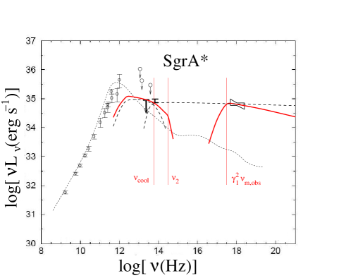
Figure 11: Two SSC models A (red) and B (black dashed) describing the April 4 2007, flare data (see Table 1, Tables 5 and 5).

Figure 12: A combined SSC and adiabatic expansion model compared to the SgrA* flare event on April 4, 2007. The data are described in Porquet et al. (2003), Dodds-Eden et al. (2009), Yusef-Zadeh et al. (2009). The 240 GHz and 43 GHz response of the NIR/X-ray flare is plotted as a solid and dashed red line, respecitvely. The probably unrelated 43 GHz response of the flare component $\xi$ with the parameters listed in Table 5 is plotted as a solid magenta line.

The SSC model that we present here for the the April 4, 2007, flare is not covered by Dodds-Eden et al. (2009). Here we cover it in more detail and take it as an example for the bright luminosity state of SgrA*. The results may be used to explain the properties of mm/sub-mm flux density variations that have been observed in several other cases (e.g. Eckart et al. 2008ab, 2009, Yusef-Zadeh et al. 2008, Marrone et al. 2009).

For the April 4, 2007 flare event our SSC model A$\gamma$ agrees with the simultaneous 3.8$\mu$m flux density, the 3$\sigma$ flux limit at 11.8$\mu$m and also the spectral index in the X-ray domain corrected for hydrogen absorption. A spectral decomposition is given in Fig. 11 and a comparison of the light curves with model A$\gamma$ and $\xi$ (see below) is displayed in Fig. 12. For the favored model A in Fig. 11 the relevant cutoff frequencies are labeled and marked with a vertical thin solid line. For model B these frequencies are all close to 7$\times$10¹³ Hz. The model data are compared to the SED of SgrA* in its quiet state. The radio to sub-mm measurements (Markoff et al. 2001; Zhao et al. 2003) are time averaged measurements, and the error bars include variable emission of up to 50%. As open black circles we show 30$\mu$m, 24.5$\mu$m and 8.6$\mu$m upper limits taken from Melia & Falcke (2001). The X-ray information is taken from Porquet et al. (2008). The short dashed line shows the quiescent model by Yuan et al. (2003).

With a magnetic field of 10 G the optically thin synchrotron spectrum extends up to $\nu_{break}$=c (3.4$\mu$m)^-1 with a spectral index of $\alpha_{synch}$=1.05. Above this the spectrum steepens until the upper synchrotron cutoff $\nu_{max}$=c (0.85$\mu$m)^-1. For a spectral index of unity, i.e. p$\sim$3, and with the assumption of a fresh injection of relativistic electroms the spectrum will steepen to a value of $p/2$$\sim$1.5. This value fully agrees with the spectral index between the infrared H- and Ks-band of $\alpha_{HK}$=1.4$\pm$0.2 which was used as an additional fitting criterion by Dodds-Eden et al. (2009).

The model can be further validated by comparing the involved electron spectral number density with values inferred from other data or different models. The value of 14$cm^{-3}keV^{-1}$ of the electron spectral number density results in number densities for the relativistic electrons of 2$\times$10⁸$cm^{-3}$. Part of the emitting particles may be due to electron/positron pairs. Integrating over the SSC source component volume of 0.2 $R_{0}$ diameter we obtain 5$\times$10^-16 M_⊙ as a lower limit to the total mass of this source component within a compact jet base that feeds an extended overall jet or outflow with a low surface brightness (Falcke & Markoff 2000, 2001, Markoff 2005, Markoff et al. 2007). If a structure of the size and density described above expands at highly relativistic velocities, it can reach the flow density of 10⁷cm^-3 (Yuan et al. 2003). This can happen on an orbital time scale of a spot which is close to the last stable orbit and on less than one flare time scale (see Fig. 10).

For the SSC model B$\gamma$ explains the NIR flux densities shortward of about 4$\mu$m through the self-Compton scattered spectrum the electron spectral number density and source component mass. This mass is four orders of magnitudes higher than for model A$\gamma$. Reaching the flow density of 10⁷cm^-3 in one flare time scale and matching the total estimated accretion rate onto SgrA* is possible as well. Still, the predicted 11.8$\mu$m flux density is well above the upper limit obtained for the April 4, 2007 flare. Therefore models in which the Ks- and L-band flux densities are produced via the self-Compton scattered spectrum are not favored.

Modeling the April 4, 2007 NIR/X-ray light curves: Dodds-Eden et al. (2009) report that the width of the X-ray flare is significantly smaller than the on of the corresponding overall L-band flare. This implies that the efficiency of producing X-ray emission was lower before and after the main part of the flare. In the framework of the evolving spot model presented in Eckart et al. (2008a) this may be explained by an evolution of the spot characteristics similar to the models presented by Hawley & Balbus (1991, 1998) and Yuan et al. (2008). The recent theoretical approach of hot spot evolution due to shearing is highlighted in Eckart et al. (2008a) and Zamaninasab et al. (2008, 2009; see also Pecháček et al., 2008). Yuan et al. (2008) explicitly solved the relativistic hydrodynamics and found initial expansion velocities of less than 0.01c close to the accretion disk followed by relativistic expansion towards the end of the flare. A compression of a single spot or merging of two spots due to differential rotation within a viscous disk may explain the different widths of the flares in the X-ray and L-band light curve. A variation of the source size $\theta$ or the peak flux density $S_{\nu}$ of the scattered synchrotron component by only 20% to 30% will result in the required significant increase or decrease in the SSC scattering efficiency, i.e. the scattered SSC X-ray flux density $S_{SSC,X-ray}$$\propto$$S_{m}^{2(\alpha+2)}$$\theta^{-2(2\alpha+3)}$. Similarly other differences between the NIR and X-ray light curves may be due to different or even varying flux density contributions and scattering efficiencies from a source component responsible for an underlying main flare and components responsible for the sub-structures.

Modeling the April 4, 2007 radio light curves: Yusef-Zadeh et al. (2009) report radio measurements that were carried out at 240 GHz (30m IRAM) during and at 43 GHz (VLA) following the April four NIR/X-ray flare. The 240 GHz data cover the entire NIR/X-ray flare event at a flux density level of about 1.2 Jy with no significant flux density variation. After a (’transatlantic’) gap in the data a strong increase and decrease of the 43 GHz flux density with a peak of about 0.4 Jy is detected. The entire 43 GHz flare has a full bottom width (at a level of about 1.1 Jy) of about 4 hours and peaks at 43 GHz about 6.5 hours past the NIR/X-ray peak.

Performing an adiabatic expansion calculation (van der Laan, 1966) based on models A$\gamma$ and B$\gamma$ using an expansion speed of 0.007c places the 43 GHz afterglow of the NIR/X-ray flare close to or even into the gap between the 100 GHz and 43 GHz measurements. We use 0.007c as a typical value close to the expansion speeds found for other SgrA* flare events for which adiabatic expansion models have been applied (see e.g. Eckart et al. 2008b, 2009, Yusef-Zadeh et al. 2008). As an example of such a calculation we show in Fig. 11 a combined SSC and adiabatic expansion model based on the data for A$\gamma$ given in Table 5. Here we assume that the 240 GHz and 43 GHz flux density level above which we have to consider the excess flare flux is at 1.08 Jy - which is at the minimum flux density level given by the data for this event. The predicted 240 GHz and 43 GHz peak brightnesses lie well within the noise of the IRAM measurements and the following 43 GHz data.

A lower expansion velocity like 0.002c gives the time delay needed to meet the bight 43 GHz flare peaking at about 12:30 UT but still fails to reproduce its high radio flux. Since measurements around this time have not given any hint for a possible NIR or X-ray counterpart for this event, it can only be explained by a low frequency flare that originated from a synchrotron component with low turnover frequency and no significant predicted NIR or X-ray flux density (like component $\xi$ given in Table 5). We therefore regard component $\xi$ as unrelated to the main NIR/X-ray flare which happened six hour earlier.

The SSC models listed in Table 5 have small source component sizes to provide a sufficient inverse Compton scattering efficiency to explain the large observed X-ray flux densities. This results in comparatively narrow light curves of the individual components and requires the observed broader flare profile to be modeled with six source components. This may explain the presence of substructure in the NIR and X-ray light curves. We place the components 1 through 6 at 5:24, 5:37, 5:51, 6:00, 6:15, and 6:21 UT with the flux ratios between them of 0.6:1:1:0.8:0.5:0.4. We also allowed components 1, 5, and 6 to be larger by $\sim 20\%$ compared to the central components. An increase in size or a decrease in flux density lowers the scattering efficiency (see above) in a way that the weaker components 1, 5, and 6 do not contribute significantly to the X-ray flare. With a spectral index of 1.05 and the dependency in scattering efficiency given above this results in an X-ray flux density ratio between the components of 0.01:1:1:0.3:0.003:0.001. This may explain the different widths of the flares in X-ray and L-band light curve and allows us to model the broader NIR flare profile.

Model B$\gamma$ in Table 5 is not well suited to explain the wings of the NIR light curve in comparison to the X-ray flare profile since the flux densities in both wavelength domains are described by the same SSC scattered spectrum. Involving steeper SSC spectra for the wings violates the 11.8$\mu$m flux density limit. Therefore the 4 April, 2007, flare event provides additional support for the assumption that - at least in this case - the NIR luminosity is due to optically thin synchrotron emission rather than SSC scattered flux.

4.4.4 SSC modeling of a weak X-ray flare

In Tables 5 and 5 we also list modeling results for the so far weakest statistically significant X-ray flare that was modeled (Eckart et al. 2002). This flare was also the first that was detected simultaneously in both the NIR and X-ray domain. The SSC model A_low which explains the NIR flux densities through the high frequency end of the associated synchrotron spectrum describes the flare successfully.

SSC models (B in Tables 5 and 5) that explain the NIR fluxes through the inverse Compton scattered part of the spectrum are strongly constrained by the NIR/X-ray spectral index determined by $\alpha_{synch}\sim 1.0$. While they do not result in a satisfactory fit of the observed data for the very bright X-ray flares (see Sect. 4.4.3), the situation for weak X-ray flares is different. Here $\alpha_{synch}$$\sim$1.3 and the corresponding electron spectral number density and source component masses are of the same order as for the SSC models A$\alpha-\gamma$. Therefore both model approaches, A_low and B_low, result in acceptable explanations for the NIR and X-ray fluxes and the spectral indices during weak flares.

4.4.5 SSC modeling of the lowest states of SgrA*

Eckart et al. (2006) have modeled the emission from SgrA* in its low flux density state. They find that the upper limits of the compact X-ray emission in the ’interim-quiescent’ (IQ), low-level luminosity states of SgrA* are consistent with a SSC model that allows for substantial contributions from both the SSC and the synchrotron part of the modeled spectrum. In these models the X-ray emission of the point source is well below 20$-$30 nJy and contributes considerably less than half of the X-ray flux density during the weak flare event reported by Eckart et al. (2004). The flux densities at a wavelength of 2.2$\mu$m are of the order of 1 to 3 mJy (see Table 2 and Figs. 8 and 9). Eckart et al. (2006) list representative SSC models for the low flux state. For their models IQ1-IQ3 the source component has a size on the order of 0.2 to 2 Schwarzschild radii with an optically thin radio/sub-mm spectral index ranging from $\alpha$$\sim$1.0 to 1.3, a value similar to the observed spectral index between the NIR and X-ray domain.

In Tables 5 and 5 we give the detailed model data for a single spot in which the MIR/NIR flux densities are accounted for by the high frequency end of the synchrotron spectrum (A_low) or by the low frequency end of the inverse self-Compton scattered spectrum (B_low). These models account for the quiescent source spectrum given by Yuan et al. (2003), as shown in Fig. 13. For model B_low the electron spectral number density value and total masses integrated over the SSC source component volume are large for a quiescent state compared to the flaring state ($\sim$3$\times$10¹¹$cm^{-3}$ and 8$\times$10^-13 M_⊙ ) and to the assumed accretion flow density of 10⁷cm^-3. Therefore model A_low is favored.

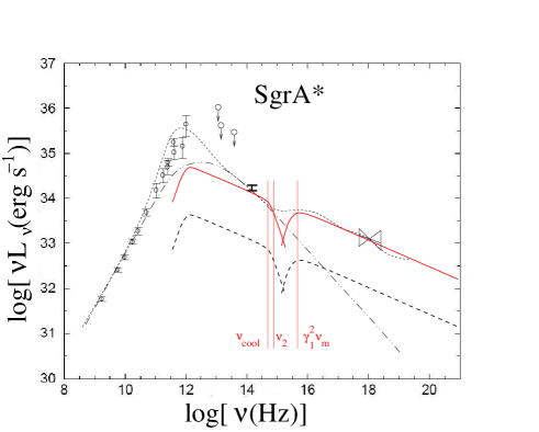
Figure 13: A single spot SSC quiescent spectrum (black dashed) and a corresponding multi-spot SSC quiescent spectrum.

As an alternative to a larger continuous disk component one may assume a continuous disk or a disk consisting of several spots with dominant source components that contribute only about 0.1 mJy (model Q_spot) to the Ks-band flux density each and have electron spectral number densities on the order of $\sim$10⁷$cm^{-3}$ and total masses integrated over small SSC source component sizes of 0.1 R_s with a diameter of a few times 10^-19 M_⊙ . Here the magnetic field strengths are comparable to those of the larger flare components, and the densities are comparable to the assumed accretion flow density of 10⁷cm^-3. In Fig. 13 - as an example - 20 spots as described by model Q_spot in Tables 5 and 5 produce a significant part of the quiescent spectrum of SgrA* in the Ks-band, as one would expect for a low level quiescent state of SgrA*. The 20 spots we used in Fig. 13 have different relativistic boosting factors as they would occur on an inclined circular orbit of a few Schwarzschild radii around the SgrA* SMBH (see Tables 5 and 5, and data in Eckart et al. 2004). In Fig. 13 relevant cutoff frequencies are labeled and marked with a vertical thin solid line. The quiescent X-ray information is taken from Baganoff et al. (2001, 2003). The short dashed line shows the quiescent model by Yuan et al. (2003). The double-dot-dashed line shows the contribution of the relativistic electrons to this quiescent model.

Therefore both a larger continuous synchrotron emitting disk or a faint disk spotted with SSC components are attractive models that may explain a possible low state of SgrA*. Any quiescent state flux density (e.g. measured in the NIR) would then be expected to be variable and polarized. High angular resolution and sensitivity - as it will be provided by the future large telescopes (ELTs) - are required to measure the quiescent state flux density contribution with sufficient precision.

4.5 Thin disk NIR luminosity

As another way to explain the Ks-band flux density especially in an assumed quiescent state of SgrA*, we explore the possible presence of a small permanent disk that radiates as a black body. Eckart et al. (2006) show that at least for the flaring state of SgrA* a disk may exist. For an optically thick disk seen at an inclination angle $i$ and radiating like a black body one finds a luminosity of

$$L_{\nu}=2.4\times 10^{-18}R_{S}^{2}cos(i)T^{8/3}\nu^{1/3}(erg/s)$$ (13)

(Peterson 1997, see also Ishibashi & Courvoisier 2009, Kishimoto et al. 2008). At infrared wavelengths and shorter the spectrum is dominated by the emission of the inner disk radii. In the NIR Ks-band 1 mJy corresponds to 3 L_⊙. For $cos(i)$$\sim$1, a Schwarzschild radius of $R_{S}$=10¹²cm, and an observing frequency of 136.364 THz for a wavelength of 2.2$\mu$m we obtain $L_{\nu}=1.235\times 10^{11}T^{8/3}(erg/s)$. So a minimum disk temperature of $T=2.6\times 10^{8}K$ is required to obtain $L_{\nu}=1L_{\odot}$. For higher temperatures one needs to introduce a surface filling factor of less than unity to explain the Ks-band emission in this model. However, one requires a high number density to have an optically thick disk. In addition the $\nu^{1/3}$ dependency is in contradiction with the steep infrared spectra that have also been observed during flares (Ghez et al. 2005ab, Eisenhauer et al. 2005, Gillessen et al. 2006, Hornstein et al. 2006, Krabbe et al. 2006). These facts make a geometrically thin and optically thick disk a very unlikely dominant contributer to explain a possible quiescent Ks-band luminosity of SgrA*.

5 Summary and conclusion

We have discussed the variable infrared and X-ray emission of SgrA* in its extreme luminosity states. We reported on Ks-band imaging of the SMBH counter part of SgrA* in its low state and investigated the structure and brightness of the central S-star cluster that surrounds the SMBH at the position of SgrA*. We have used three independent methods to remove or strongly suppress the flux density contributions of stars in the central 2” diameter region around SgrA*. All methods revealed faint extended emission around the SgrA* position. De-reddened with $A_{K}$=2.8 the peak emission of the extended S-star cluster is about 1.3 mJy within one resolution element, corresponding to a surface flux density of about 0.5 Jy (dereddened) per square arcsecond. For the dataset taken on 23 September 2004 no NIR counterpart of SgrA* was detected with a flux density limit of about 2 mJy (dereddened). For 30 August 2004 we find a NIR counterpart of SgrA* with a dereddened flux density of about 4 mJy. We find that the luminosity during the low state can most likely be accounted for by synchrotron emission from a continuous or spotted accretion disk. In this case we expect the possible quiescent source associated with SgrA* to be significantly polarized.

Steep spectral indices observed in the NIR wavelength domain may reflect the presence of typical cutoff frequencies. In addition to the cooling break $\nu_{break}$ as discussed in Sect. 4.4.1 there may be a cutoff in the relativistic electron spectrum at work (e.g. Eckart et al. 2006a, Liu et al. 2006). This will result in a modulation of the intrinsically flat spectra with an exponential cutoff proportional to $exp[-(\lambda_{0}/\lambda)^{0.5}]$ (see e.g. Bregman 1985, and Bogdan & Schlickeiser 1985) and a cutoff wavelength $\lambda_{0}$ in the infrared. If $\lambda_{0}$ lies in the 4-8$\mu$m wavelength range (Eckart et al. 2006a), the variation in the spectral index is on the order of $\Delta\alpha$$\sim$1.0. In a number of extragalactic jets these cutoffs have been observed to be relevant in the NIR wavelength domain (3C 293: Floyd et al. 2006, M87: Perlman et al. 2001; Perlman & Wilson 2005; 3C 273: Jester et al. 2001, 2005). In these sources the cutoff frequency at which synchrotron losses become dominant is $\nu_{jet,break}$=4$\times$10¹³Hz (or 7.5$\mu$m wavelength), which is remarkably similar to what may be required in the case of the Galactic center (Eckart et al. 2006a). For SgrA* such a cutoff can quite naturally explain the steep NIR spectral indices reported by (Eisenhauer et al. 2005, Gillessen et al. 2006, Krabbe et al. 2006) despite the low upper flux density limits in the MIR.

For the three brightest X-ray flares the SSC emission from THz peaked source components can fully account for the observed flux density variations observed in the NIR and X-ray domain. Here models in which the MIR/NIR flux density contributions are due to the high frequency tail of the associated synchrotron spectrum are favored (models A in Tables 5 and 5). Combined with the source component size of 0.2-0.3 $R_{0}$ and relativistic expansion within or towards the end of the flare, the spectral energy densities of relativistic electrons are compatible with the electron number density derived for the accretion flow at 10 R_s distance and the estimated upper limits of the mass accretion rate onto SgrA*. For the weak X-ray flare first discussed by Eckart et al. (2004) these boundary conditions are fulfilled for both model approaches (A and B). For model A_low we expect significant polarization of the NIR flux density, whereas for model B_low the scattering process should lead to a significantly lower degree of polarization.

For the 4 April 2007 flare our favored model A$\gamma$ of the peak fluxes meets the 11.8$\mu$m 3$\sigma$ limit and is only by 1$\sigma$ off the expected flux density at 3.8$\mu$m wavelength. In the X-ray domain it matches the mean flux exactly and the spectral slope by 0.8$\sigma$. Giving these four quantities the same weight we obtain a reduced $\chi^{2}_{red}$ value of $\chi^{2}_{red}$=10.7/d.o.f=3.7. The X-ray data cover a comparatively large and rather densely sampled spectral range. We get $\chi^{2}_{red}$$\leq$2 if the X-ray information is weighted higher by a factor of two or more (see Porquet et al. 2008, Dodds-Eden et al. 2009). A  $\chi^{2}$-based comparison of different single component emission models over a large wavelength range (radio or infrared till X-ray) is, however, only of limited value. More adequate physical models of the compact emission from SgrA* contain on some level contributions from several source components, like the hot-spot/disk (Eckart et al. 2006b, Broderick & Loeb 2006) or multi-spot models (Eckart et al. 2008a , see also Pecháček et al., 2008), the spiral arm models (Karas et al. 2007, Falanga et al. 2007), the more elaborate evolving hot-spot model by (Yuan et al. 2008), or the jet/jet-base models (Falcke & Markoff 2000, 2001, Markoff 2005, Markoff et al. 2007). This implies that in addition to a possible dominant emission component, secondary source or spectral components will contribute to the flux and spectral index information in the different wavelength bands across the electromagnetic spectrum. This complicates the comparison of different models. Distinguishing between emission mechanisms requires more work on detailed flare modeling, using time dependent dense flux density sampling across a broad frequency band, preferentially including polarization and spatial information.

Here we presented a new SSC model for the flare event on April 4, 2007 that accounts for the available simultaneous peak flux density and spectral index information. Variations in the SSC scattering explain that the flare profile in the X-ray domain is narrower than that at NIR wavelengths. This suggests at least for this flare event that models in which the NIR flares are due to optically thin synchrotron radiation rather than inverse Compton scattered light are preferred. In general models in which the MIR/NIR flux densities are explained through the low frequency tail of the inverse Compton scattered spectrum are disfavored. They result in higher masses for the emitting sources.

We conclude that both weak and bright flares from SgrA* can be explained by the synchrotron self-Compton mechanism. This emission mechanism may explain the flare activity over up to two orders in magnitude in the NIR or X-ray flux density and over six orders of magnitude in frequency. No other dominant emission mechanisms are required. Densities of relativistic electrons of a few times 10⁷ cm${}^{-}3$ (comparable to what is derived from X-ray data on a 1000 Schwarzschild radii scale) are also required close to the SgrA* black hole to explain the flare emission.

The variable synchrotron emission may be limited at short wavelengths by a NIR cutoff (cooling break) due to synchrotron losses. The self-Compton scattered spectrum may be limited at the longest wavelengths by the low energy cutoff in the relativistic electron distribution. If future sub-mm and X-ray obervations allow for a simultaneous detection of the THz turnover frequency ($\nu_{m}$) and a low energy cutoff of the SSC spectrum ($\nu_{SSC,upper}$), information on the low energy cutoff in the relativistic electron distribution can be obtained via $\gamma$₁²$\sim$$\nu_{SSC,upper}$$\nu_{m}^{-1}$. In a few years further polarimetric NIR observations at high angular resolution and sensitivity will help to distinguish between the importance of the different emission mechanisms in the low state of SgrA*. Interferometric observations in the near-infrared using GRAVITY at the VLTI (Eisenhauer et al. 2008, Straubmeier et al. 2008, Zamaninasab et al. 2009) and in the mm-wavelength domain (e.g. Fish et al. 2009, Doeleman et al. 2009) will be important to understand the emission from SgrA*.

Alexander, T.; Hopman, C., 2009, ApJ 697, 1861

Bondi, H., 1952, MNRAS 112, 195

Baganoff, F.K., Bautz, M.W., Brandt, W.N., et al. 2001, Nature, 413, 45

Baganoff, F. K., et al., 2002, 201st AAS Meeting, #31.08; Bulletin of the American Astronomical Society, Vol. 34, 1153

Baganoff, F. K., Maeda, Y., Morris, M., et al. 2003, ApJ 591, 891

Bahcall, J. N.; Wolf, R. A., 1976, ApJ 209, 214

Bélanger, G.; Terrier, R.; de Jager, O. C.; Goldwurm, A.; Melia, F., 2006, JPhCS 54, 420

Blum, R. D.; Sellgren, K.; Depoy, D. L., 1996, ApJ 470, 864

Bogdan, T.J., & Schlickeiser, R., 1985, å, 143, 23

Bower, G. C., Falcke, H., Herrnstein, R. M., Zhao, J., Goss, W. M., & Backer, D. C. 2004, Science, 304, 704

Bregman, J.N., 1985, AJ, 288, 32

Broderick, A.E., Loeb, A., 2006, MNRAS 367, 905

Buchholz, R. M.; Schödel, R.; Eckart, A, 2009, A&A 499, 483

Cuadra, J.; Nayakshin, S., 2006, JPhCS 54, 436

Cuadra, J.; Nayakshin, S.; Martins, F., 2008, MNRAS 383, 458

Diolaiti, E. Bendinelli, O., Bonaccini, D., Close, L., Currie, D., Parmeggiani, G., A&AS 147, 335-346, 2000

Do, T.; Ghez, A.M.; Morris, M.R.; Yelda, S.; Meyer, L.; Lu, J.R.; Hornstein, S.D.; Matthews, K., 2009a, ApJ 691, 1021.

Do, T.; Ghez, A.M.; Morris, M.R.; Lu, J.R.; Matthews, K.; Yelda, S.; Larkin, J., 2009b, 2009arXiv0908.0311D

Doeleman, S.S.; Fish, V.L.; Broderick, A.E.; Loeb, A.; Rogers, A.E.E., 2009, ApJ 695, 59D

Dodds-Eden, K.; Porquet, D.; Trap, G.; Quataert, E.; Haubois, X.; Gillessen, S.; and 19 coauthors, 2009, ApJ 698, 676

Eckart, A.; Duhoux, P. R. M. 1990, ASPC, 14, 336

Eckart, A. & Genzel, R. 1996, Nature 383, 415

Eckart, A., Genzel, R., Ott, T. and Schödel, R. 2002, MNRAS, 331, 917

Eckart, A.; Moultaka, J.; Viehmann, T.; Straubmeier, C.; Mouawad, N.; Genzel, R.; Ott, T.; Schödel, R.; Baganoff, F. K.; Morris, M. R, 2003, ANS 324, 557

Eckart, A.; Baganoff, F. K.; Morris, M.; and 11 coauthors, 2004, A&A 427, 1

Eckart, A.; Baganoff, F. K.; Schödel, R.; Morris, M.; Genzel, R.; Bower, G. C.; Marrone, D.; et al. 2006a, A&A 450, 535

Eckart, A.; Schödel, R.; Meyer, L.; Trippe, S.; Ott, T.; Genzel, R., 2006b, A&A 455, 1

Eckart, A.; Baganoff, F. K.; Zamaninasab, M.; Morris, M. R.; Schödel, R.; and 16 coauthors, 2008a, A&A 479, 625

Eckart, A.; Schödel, R.; Garcia-Marin, M.; Witzel, G.; Weiss, A.; Baganoff, F. K.; Morris, M. R.; Bertram, T.; Dovciak, M.; Duschl, W. J.; and 21 coauthors, 2008b, A&A 492, 337

Eckart, A.; Baganoff, F. K.; Morris, M. R.; Kunneriath, D.; Zamaninasab, M.; Witzel, G.; Schödel, R.; Garcia-Marin, M.; Meyer, L.; Bower, G. C.; and 10 coauthors, 2009, A&A 500, 935.

Eisenhauer, F.; Schödel, R.; Genzel, R.; Ott, T.; Tecza, M.; Abuter, R.; Eckart, A.; Alexander, T., 2003, ApJ 597, L121

Eisenhauer, F.; Genzel, R.; Alexander, T.; Abuter, R.; Paumard, T.; Ott, T.; ; and 15 coauthors, 2005, ApJ 628, 246

Eisenhauer, F.; Perrin, G.; Brandner, W.; Straubmeier, C.; Richichi, A.; Gillessen, S.; Berger, J. P.; Hippler, S.; Eckart, A.; Schöller, M.; and 38 coauthors, 2008, SPIE 7013, 69

Fish, V.L.; Doeleman, S.S.; Broderick, A.E.; Loeb, A.; Rogers, A.E.E., 2009, ApJ 706, 1353

Falanga, M., Melia, F., Tagger, M., Goldwurm, A., Belanger, G., 2007, ApJ 662, L15

Falcke, H.; Markoff, S.; Fender, R., 2001, AGM 18, 107

Falcke, H.; Markoff, S., 2000, A&A 362, 113

Floyd D.J.E., Eric Perlman, E., Leahy, J.P., and 5 coauthors, 2006, ApJ 639, 23

Genzel, T., Eckart, A., Ott, T. & Eisenhauer, MNRAS 1997, 291, 219

Genzel, R., Pichon, C., Eckart, A., Gerhard, O.E., Ott, T. 2000, MNRAS 317, 348

Genzel, R., Schödel, R., Ott, T., et al. 2003, Nature, 425, 934

Gezari, S., Ghez, A. M., Becklin, E. E., Larkin, J., McLean, I. S., Morris, M., ApJ 576, 790, 2002

Ghez, A., Klein, B.L., Morris, M. & Becklin, E.E. 1998, ApJ, 509, 678

Ghez, A., Morris, M., Becklin, E.E., Tanner, A. & Kremenek, T. 2000, Nature 407, 349

Ghez, A. M., Duchéne, G., Matthews, K., et al. 2003, ApJ, 586, L127

Ghez, A.M., Wright, S.A., Matthews, K., et al. 2004a, ApJ 601, 159

Ghez, A.M., Hornstein, S.D., Bouchez, A., Le Mignant, D., Lu, J., Matthews, K., Morris, M., Wizinowich, P., Becklin, E.E., 2004b, AAS 205, 2406

Ghez, A.M., Salim, S., Hornstein, S. D., Tanner, A., Lu, J. R., Morris, M., Becklin, E. E., Duchêne, G., 2005a, ApJ 620, 744

Ghez, A. M.; Hornstein, S. D.; Lu, J. R.; Bouchez, A.; Le Mignant, D.; van Dam, M. A.; Wizinowich, P.; Matthews, K.; Morris, M.; Becklin, E. E.; and 7 coauthors, 2005b, ApJ 635, 1087

Gillessen, S.; Eisenhauer, F.; Trippe, S.; Alexander, T.; Genzel, R.; Martins, F.; Ott, T., 2009, ApJ 692, 1075

Gillessen, S.; Eisenhauer, F.; Quataert, E.; Genzel, R.; Paumard, T.; Trippe, S.; Ott, T.; Abuter, R.; Eckart, A.; and 4 coauthors, 2006, ApJ 640, L163

Goldwurm, A., Brion, E., Goldoni, P. et al. 2003, ApJ, 584, 751

Gould, R.J., 1979, A&A 76, 306

Hawley, J.F.; Balbus, S.A., 1991, ApJ 376, 223

Hawley, J.F.; Stone, J.M., 1998, ApJ 501, 758,

Hornstein, S.D.; Ghez, A.M.; Tanner, A.; Morris, M.; Becklin, E. E.; Wizinowich, P., 2002, ApJ 577, L9

Hornstein, S.D., et al., 2006, JPhCS 54, 399

Hornstein, S. D., Matthews, K., Ghez, A. M., Lu, J. R., Morris, M., Becklin, E. E., Rafelski, M., & Baganoff, F. K. 2007, ApJ, 667, 900

Igumenshchev, I.V., 2002, ApJ 577, 31

Ishibashi, W.; Courvoisier, T. J.-L., 2009, A&A 495, 113

Jester, S., Röser, H.-J., Meisenheimer, K., & Perley, R. 2005, A&A, 431, 477

Jester, S., Röser, H.-J., Meisenheimer, K., Perley, R., & Conway, R. 2001, A&A, 373, 447

Karas, V., Dovciak, M., Eckart, A., Meyer, L., 2007, Proceedings of the Workshop on the Black Holes and Neutron Stars, eds. S. Hledik and Z. Stuchlik, 19-21 September 2007 (Silesian University, Opava), pp. 99-108, arXiv:0709.3836

Kardashev, N.S., 1962, SvA 6, 317

Kishimoto, M.; Antonucci, R.; Blaes, O.; Lawrence, A.; Boisson, C.; Albrecht, M.; Leipski, C., 2008, Nature 454, 492

Krabbe, A.; Iserlohe, C.; Larkin, J. E.; Barczys, M.; McElwain, M.; Weiss, J.; Wright, S. A.; Quirrenbach, A. 2006, ApJ 642, L145

Lightman, A. P., & Shapiro, S. L. 1977, ApJ, 211, 244

Liu, S.; Petrosian, V.; Melia, F; Fryer, C, 2006, ApJ 648, 1020

Lucy, L. B. 1974, AJ, 79, L745

Mahadevan, R. & Quataert, E. 1997, ApJ, 490, 605

Markoff, S., Falcke, H., Yuan, F. & Biermann, P.L. 2001, A&A, 379, L13

Markoff, S., 2005, ApJ 618, L103

Markoff, S.; Bower, G.C.; Falcke, H., 2007, MNRAS 379, 1519

Marrone, D.P.; Moran, J.M.; Zhao, J.-H.; Rao, R. 2007, ApJ 654, L57

Marrone, D. P.; Baganoff, F. K.; Morris, M.; and 14 coauthors, 2008, ApJ 682, 373

Marscher, A.P. 1983, ApJ, 264, 296

Melia, F. & Falcke, H. 2001, ARA&A 39, 309

Meyer, L., Eckart, A., Schödel, R., Dovciak, M., Karas, V., Duschl, W.J., 2007, A&A 473, 707

Meyer, L., Eckart, A., Schödel, R., Duschl, W. J., Muciz, K., Dovciak, M., Karas, V., 2006a, A&A 460, 15

Meyer, L., Schödel, R., Eckart, A., Karas, V., Dovciak, M., Duschl, W. J., 2006b, A&A 458, L25

Murphy, B. W., Cohn, H. N., & Durisen, R. H. 1991, ApJ, 370, 60

Nayakshin, S.; Sunyaev, R., 2003, MNRAS 343, L15

Özel, F., Psaltis, D., & Narayan, R. 2000, ApJ, 541, 234

Ott, T.; Eckart, A.; Genzel, R., 1999, ApJ 523, 248

Page, K.L.; Reeves, J.N.; O’Brien, P.T.; Turner, M.J. L.; Worrall, D.M., 2004, MNRAS 353, 133

Pecháček, T., Karas, V., Czerny, B., 2008, A&A 487, 815

Perlman, E. S., Biretta, J. A., Sparks, W. B., Macchetto, F. D., & Leahy, J. P. 2001, ApJ, 551, 206

Perlman, E. S., & Wilson, A. S. 2005, ApJ, 627, 140

Peterson, B.M., 1997, ’An introduction to active galactic nuclei’, p. 44, Cambridge University Press

Porquet, D., Predehl, P., Aschenbach, et al. 2003, A&A 407, L17

Porquet, D.; Grosso, N.; Predehl, P.; Hasinger, G.; Yusef-Zadeh, F.; and 11 coauthors; 2008, A&A 488, 549

Quataert, E. 2002, ApJ, 575, 855

Quataert, E., Astron. Nachr., Vol. 324, No. S1 (2003), Special Supplement ”The central 300 parsecs of the Milky Way”, Eds. A. Cotera, H. Falcke, T. R. Geballe, S. Markoff, p. 435 (astro-ph/0304099)

Reid, Mark J., 1993, ARA&A 31, 345

Straubmeier, Christian; Eisenhauer, Frank; Perrin, Guy; Brandner, Wolfgang; Eckart, Andreas, 2008, SPIE 7013, 93

Schödel, R.; Merritt, D.; Eckart, A., 2009, A&A 502 91

Schödel, R.; Eckart, A.; Alexander, T.; Merritt, D.; Genzel, R.; Sternberg, A.; Meyer, L.; Kul, F.; Moultaka, J.; Ott, T.; Straubmeier, C. 2007, A&A 469, 125

Schödel, R., Genzel, R., Ott, et al. 2003, ApJ, 596, 1015

Schödel, R., Ott, T., Genzel, R. et al. 2002, Nature, 419, 694

Scoville, N. Z.; Stolovy, S. R.; Rieke, M.; Christopher, M.; Yusef-Zadeh, F., 2003, ApJ 594, 294

Tanner, A.; Ghez, A. M.; Morris, M.; Becklin, E. E.; Cotera, A.; and 3 coauthors, 2002, ApJ 575, 860

Tanner, A.; Ghez, A. M.; Morris, M. R.; Christou, J. C., 2005, ApJ 624, 742

van der Laan, H., 1966, Nature 211, 1131

Yuan, F., Quataert, E., & Narayan, R. 2003, ApJ, 598, 301

Yuan, F., 2006, JPhCS 54, 427

Yuan, F., Lin, J.; Wu, K.; Ho, Luis C., 2008, MNRAS 395, 2183

Yusef-Zadeh, F., Roberts, D., Wardle, M., Heinke, C. O., Bower, G. C., 2006a, ApJ 650, 189

Yusef-Zadeh, F., et al., 2006b, ApJ 644, 198

Yusef-Zadeh, F.; Wardle, M.; Cotton, W. D.; Heinke, C. O.; Roberts, D. A., 2007, ApJ 668, L47

Yusef-Zadeh, F.; Wardle, M.; Heinke, C.; Dowell, C. D.; Roberts, D.; Baganoff, F. K.; Bower, G. C., 2008, ApJ 682, 361

Yusef-Zadeh, F.; Bushouse, H.; Wardle, M.; Heinke, C.; Roberts, D. A.; and 16 coauthors, 2009, 2009arXiv0907.3786Y

Zamaninasab, M., Eckart, A., Meyer, L., Schödel, R., Dovciak, M., Karas, V., Kunneriath, D., Witzel, G., Giessuebel, R., König, S., Straubmeier, C., Zensus, A., 2008, Proc. of a conference on ’Astrophysics at High Angular Resolution (AHAR 08)’ held 21-25 April 2008 in Bad Honnef, Germany, 2008, JPhCS 131, 12008

Zamaninasab, M.; Eckart, A.; Witzel, G.; Dovciak, M.; Karas, V.; Giessuebel, R. Schödel R.; Bremer, M.; Garcia-Marin, M.; Kunneriath, D.; Muzic, K.; and 4 coauthors 2009, arXiv0911.4659, A&A in press

Zhao, J.-H., Young, K.H., Herrnstein, R.M., Ho, P.T.P., Tsutsumi, T., Lo, K.Y., Goss, W.M. & Bower, G.C., 2003, ApJL, 586, L29.