First- and second-order phase transitions in Ising models on small world networks, simulations and comparison with an effective field theory

Abstract

We perform simulations of random Ising models defined over small-world networks and we check the validity and the level of approximation of a recently proposed effective field theory. Simulations confirm a rich scenario with the presence of multicritical points with first- or second-order phase transitions. In particular, for second-order phase transitions, independently of the dimension $d_{0}$ of the underlying lattice, the exact predictions of the theory in the paramagnetic regions, such as the location of critical surfaces and correlation functions, are verified. Quite interestingly, we verify that the Edward-Anderson model with $d_{0}=2$ is not thermodynamically stable under graph-noise.

I Introduction

Disordered systems represent one of the most important fields of statistical mechanics. Disorder is at the base of many interesting phenomena whose understanding is often far from being trivial or immediate. Its use varies from applications in condensed matter physics to computer science and, more recently, to the broad range of natural, artificial, and social networks. One of the most important analytical tool to study disordered systems is represented by suitable mean-field theories. Originally developed to understand spin glass models, the replica method (RM) and the cavity method (CM) are nowadays largely used in many other fields of statistical physics and computer science and represent the most powerful analytical methods to investigate the intricate nature of the spin glass and other disordered phases Parisi ; MezardP ; Diluted .

Among disordered models whose dimensionality - in a broad sense - can be considered infinite MOIII , one can single out a “hierarchical” family of models of increasing difficulty such as: fully connected models (corresponding to infinite connectivity in the thermodynamic limit) like the Sherrington-Kirkpatrick model SK , finite connectivity models like the Viana-Bray model VB , and models defined over small-world networks Watts ; Barrat . This latter class of models has been introduced in recent years and represents an important development in modeling more realistic situations in which the spins, besides interacting through a random finite connectivity, distributed according to some given distribution with average degree $c$, interact also through short-range connections. In other words, small-world models constitute an interplay between purely random and regular finite-dimensional models. It is known that, despite the underlying finite dimensionality $d_{0}$ present in these kind of graphs, in the thermodynamic limit, models defined on them manifest a mean field behavior. This fact, far from being trivial, to be rigorously proved, may lead to hope that the RM or the CM could be used to solve small-world models. Indeed such methods have been already successfully exploited in Niko ; Niko2 ; Bolle for $d_{0}=1$ small-world models defined upon adding a Poisson distributed random connectivity $c$ to the underlying regular one-dimensional chain. However, if we take a look at the mathematical structure of these methods we recognize the following. For what concerns the RM, we need to know analytically the two leading eigenvectors of the transfer matrix of the Ising model without the shortcuts but immersed in a random external field; whereas for what concerns the CM, it is essential that the underlying graph $\mathcal{L}_{0}$ had a tree-like structure, i.e., no loops, at least in the thermodynamic limit. As a consequence, both methods seem hardly applicable to small-world models if $d_{0}>1$. The effective field theory we have recently developed in SW , based on mapping a generic random model onto a non random one (the “pure model”) MOI ; MOII ; MOIII is instead applicable to these models. In fact, though this theory is able to give exact answers only in the paramagnetic (P) regions, there is no limitation in the underlying dimension $d_{0}$. Whereas the theory can be fully treated analytically for $d_{0}\leq 1$, for $d_{0}>1$, we can still apply it semi-analytically . All we need to apply the theory is to solve - analytically or numerically - the pure model in $d_{0}$ dimension in the absence of the random shortcuts and in the presence of a uniform external field. The values of a certain observable $\mathrm{O}_{0}$ so obtained una tantum will be then used to get the corresponding value $\mathrm{O}$ for the model in the presence of the shortcuts and for any choice of the disorder parameters (couplings and connectivity). This feature, together with the fact that the effective field equations of the theory have a very simple structure and a more immediate physical interpretation compared to the equations of the RM method (in which the introduction of several coupled auxiliary fields is necessary), makes this effective field theory particularly interesting to all those applications in which $d_{0}>1$ or else the number of parameters of the model is high. Of course one has to pay such an advantage with the impossibility to get exact results out of the P region. However, as we shall show in this paper, also in the other regions of the phase diagram the theory succeeds in giving effective approximations allowing us to obtain important insights on the frozen states, even if we do not have a direct access to them, as instead the RM or the CM could do, if they were applicable also to models with loops.

In this paper we consider random Ising models defined over small-world networks having an underlying regular lattice $\mathcal{L}_{0}$ of dimension $d_{0}=1,2,3$. Given the initial lattice $\mathcal{L}_{0}$ with $N$ sites, we build the small-world network by adding $cN/2$ links uniformly spread over $\mathcal{L}_{0}$. This implies that at each site, besides the $2d_{0}$ neighbors, there are additional long-range neighbors whose number is distributed according to a Poisson distribution with average $c$. Interactions act via a coupling $J_{0}$ for the $2d_{0}$ short-range neighbors and via a further coupling $J$ for the other long-range neighbors. This way of building a small-world network is different from the re-wiring method of Watts and StrogatzWatts (in which the number of shortcuts per site is also Poissonian distributed) and it is more convenient for analytical calculations. However, just by using the effective field theory at the base of this paper, it is possible to deal with the similar re-wiring small-world models as well, and to show rigorously that the critical behavior of the two kind of models is identical SF .

By using Monte Carlo (MC) simulations we check the predictions of the effective field theory for the critical surfaces, the susceptibility, the average magnetization and the two point connected correlation function as a function of the Euclidean distance $r$ defined on $\mathcal{L}_{0}$.

The ferromagnetic Ising model (both $J$ and $J_{0}$ positive) on small-world networks has been extensively studied Barrat ; gitterman ; pekalski ; lopes ; herrero2002 ; Hastings2 . However, of remarkable interest, for both its theoretical and practical implications, is the case with negative short-range antiferromagnetic coupling, $J_{0}<0$. The anti-ferromagnetic Ising model on small world networks was studied in herrero2008 for the case where there is only one antiferromagnetic coupling constant ($J_{0}=J$), but, apart from the fully connected case Skantzos , no attention has been paid to the fact that, in the more general situation, may exist multicritical points with first- and second-order phase transition. In fact, when $J_{0}<0$ and $J>0$, the effective field theory predicts two critical temperatures with first or second-order phase transitions separating two P regions. In this case, simulation results show large fluctuations and a rather slow approach to the thermodynamic limit, confirming the slow dynamics of the frustrated system and the importance to have analytical or semi-analytical frustrated-free tools to investigate these models. Quite interestingly, the model with given couplings $J_{0}$ and $J$, and slightly different values of the connectivity $c$, can show drastically different phase diagrams either showing two ferromagnetic (F) phase transitions or a single spin-glass (SG) phase transition. In the case of first-order phase transitions the magnetization discontinuity is not exactly predicted by the theory but simulation results show clearly the signature of a discontinuity for both the F and SG order parameters in correspondence of the theoretical P-SG critical temperature. Furthermore, we see good agreement of the susceptibility predictions in the P phase. We also consider a two-dimensional modified Edwards-Anderson modeledwards with added long-range shortcuts. This is a special case where besides the connectivity disorder there is also disorder on the value of the short-range coupling. As predicted by the theory, simulations confirm that any infinitesimal addition of shortcuts leads the system to have a finite temperature P-SG phase transition which coincides with the theoretical one.

The paper is organized as follows. In Secs. II and III we recall the definition of the small-world models and the method, which mainly consists in finding the solution of the self-consistent equation (13) and minimizing the effective free energy (31). In Sec. IV we report our MC simulations for several interesting cases selected for comparison with the theoretical predictions. Finally, in Sec. V some conclusions are drawn.

II Small world models

We consider random Ising models constructed by super-imposing random graphs with finite average connectivity onto some given lattice $\mathcal{L}_{0}$ whose set of bonds $(i,j)$ and dimension will be indicated by $\Gamma_{0}$ and $d_{0}$, respectively. Given an Ising model - shortly the pure model - of $N$ spins coupled over $\mathcal{L}_{0}$ through a coupling $J_{0}$ and with Hamiltonian

$$H_{0}{\buildrel\;def\;\over{=}}-J_{0}\sum_{(i,j)\in\Gamma_{0}}\sigma_{i}\sigma_{j}-h\sum_{i}\sigma_{i},$$ (1)

and given an ensemble $\mathcal{C}$ of unconstrained random graphs $\bm{c}$, $\bm{c}\in\mathcal{C}$, whose bonds are determined by the adjacency matrix elements $c_{i,j}=0,1$, we define the corresponding small-world model - shortly the random model - as described by the following Hamiltonian

$$H_{\bm{c};\bm{J}}{\buildrel\;def\;\over{=}}H_{0}-\sum_{i<j}c_{ij}{J}_{ij}\sigma_{i}\sigma_{j},$$ (2)

the free energy $F$ and the averages $\overline{\langle\mathop{O}\rangle^{l}}$ being defined in the usual (quenched) way as

$$-\beta F{\buildrel\;def\;\over{=}}\sum_{\bm{c}\in\mathcal{C}}P(\bm{c})\int d\mathcal{P}\left(\{{J}_{i,j}\}\right)\ln\left(Z_{\bm{c};\bm{J}}\right),$$ (3)

and (in the following a bar notation $\bar{\cdot}$ indicates the two independent averages over the graph and couplings realizations)

$$\overline{\langle\mathop{O}\rangle^{l}}{\buildrel\;def\;\over{=}}\sum_{\bm{c}\in\mathcal{C}}P(\bm{c})\int d\mathcal{P}\left(\{{J}_{i,j}\}\right)\langle\mathop{O}\rangle^{l},\quad l=1,2$$ (4)

where $Z_{\bm{c};\bm{J}}$ is the partition function of the quenched system

$$Z_{\bm{c};\bm{J}}=\sum_{\{\sigma_{i}\}}e^{-\beta H_{\bm{c};\bm{J}}\left(\{\sigma_{i}\}\}\right)},$$ (5)

$\langle\mathop{O}\rangle_{\bm{c};\bm{J}}$ the Boltzmann-average of the quenched system (note that $\langle\mathop{O}\rangle_{\bm{c};\bm{J}}$ depends on the given realization of the ${J}$’s and of $\bm{c}$: $\langle\mathop{O}\rangle=\langle\mathop{O}\rangle_{\bm{c};\bm{J}}$; for shortness we will often omit to write these dependencies)

$$\langle\mathop{O}\rangle{\buildrel\;def\;\over{=}}\frac{\sum_{\{\sigma_{i}\}}\mathop{O}_{\bm{c};\bm{J}}e^{-\beta H_{\bm{c};\bm{J}}\left(\{\sigma_{i}\}\right)}}{Z_{\bm{c};\bm{J}}},$$ (6)

and $d\mathcal{P}\left(\{{J}_{i,j}\}\right)$ and $P(\bm{c})$ are two product measures given in terms of two normalized measures $d\mu(J_{i,j})\geq 0$ and $p(c_{i,j})\geq 0$, respectively:

$$d\mathcal{P}\left(\{{J}_{i,j}\}\right){\buildrel\;def\;\over{=}}\prod_{(i,j),i<j}d\mu\left({J}_{i,j}\right),\quad\int d\mu\left({J}_{i,j}\right)=1,$$ (7)

$$P(\bm{c}){\buildrel\;def\;\over{=}}\prod_{(i,j),i<j}p(c_{i,j}),\quad\sum_{c_{i,j}=0,1}p(c_{i,j})=1.$$ (8)

The variables $c_{i,j}\in\{0,1\}$ specify whether a “long-range” bond between the sites $i$ and $j$ is present ($c_{i,j}=1$) or absent ($c_{i,j}=0$), whereas the $J_{i,j}$’s are the random variables of the given bond $(i,j)$. For the $c_{i,j}$’s, we shall consider the following distribution

$$p(c_{ij})=\frac{c}{N}\delta_{c_{ij},1}+\left(1-\frac{c}{N}\right)\delta_{c_{ij},0},$$ (9)

where $c>0$. This choice leads in the thermodynamic limit $N\to\infty$ to a number of long range connections per site distributed according to a Poisson law with mean connectivity $c$.

In this paper for the $J_{i,j}$’s we will assume the distribution

$$\frac{d\mu\left({J}_{i,j}\right)}{d{J}_{i,j}}=\delta\left({J}_{i,j}-J\right),$$ (10)

For the short-range nearest-neighbor coupling, $J_{0}$ we will consider the distribution,

$$\frac{d\mu\left(J_{0}\right)}{dJ_{0}}=\delta(J_{0}-a),$$ (11)

except in the last case studied, the modified Edwards-Anderson model, where we consider,

$$\frac{d\mu_{0}(J_{0})}{dJ_{0}}=\frac{1}{2}\delta(J_{0}-a)+\frac{1}{2}\delta(J_{0}+a).$$ (12)

III An effective field theory

Depending on the temperature T, and on the parameters of the probability distributions, $d\mu$ and $p(c_{i,j})$, the random model may stably stay either in the paramagnetic (P), in the ferromagnetic (F), or in the spin glass (SG) phase. In our approach for the F and SG phases there are two natural order parameters that will be indicated by $m^{(\mathrm{F})}$ and $m^{(\mathrm{SG})}$. Similarly, for any correlation function, quadratic or not, there are two natural quantities indicated by $C^{(\mathrm{F})}$ and $C^{(\mathrm{SG})}$, and that in turn will be calculated in terms of $m^{(\mathrm{F})}$ and $m^{(\mathrm{SG})}$, respectively. To avoid confusion, it should be kept in mind that in our approach, for any observable $\mathcal{O}$ there are - in principle - always two solutions that we label as F and SG, but, for any temperature, only one of the two solutions is stable and useful in the thermodynamic limit.

In the following, we will use the label $\mathop{}_{0}$ to specify that we are referring to the pure model with Hamiltonian (1). Let $m_{0}(\beta J_{0},\beta h)$ be the stable magnetization of the pure model with coupling $J_{0}$ and in the presence of a uniform external field $h$ at inverse temperature $\beta$. Then, the order parameters $m^{(\Sigma)}$, $\Sigma$=F,SG, satisfy the following self-consistent decoupled equations

$$m^{(\Sigma)}=m_{0}(\beta J_{0}^{(\Sigma)},\beta J^{(\Sigma)}m^{(\Sigma)}+\beta h),$$ (13)

where the effective couplings $J^{(\mathrm{F})}$, $J^{(\mathrm{SG})}$, $J_{0}^{(\mathrm{F})}$ and $J_{0}^{(\mathrm{SG})}$ are given by

$$\beta J^{(\mathrm{F})}=c\int d\mu(J_{i,j})\tanh(\beta J_{i,j}),$$ (14)

$$\beta J^{(\mathrm{SG})}=c\int d\mu(J_{i,j})\tanh^{2}(\beta J_{i,j}).$$ (15)

For a constant short-range coupling distributed as in (11)

$$\begin{array}[]{l l l}J_{0}^{(\mathrm{F})}&=&a\\ &&\\ \beta J_{0}^{(\mathrm{SG})}&=&\tanh^{-1}(\tanh^{2}(\beta a)).\end{array}$$ (19)

and for the bimodal distribution (12),

$$\begin{array}[]{l l l}J_{0}^{(\mathrm{F})}&=&0\\ &&\\ \beta J_{0}^{SG}&=&\tanh^{-1}(\tanh^{2}(\beta a))\end{array}$$ (23)

For the correlation functions we have ${{C}}^{(\Sigma)}$, $\Sigma$=F,SG, where

$${{C}}^{(\Sigma)}={{C}}_{0}(\beta J_{0}^{(\Sigma)},\beta J^{(\Sigma)}m^{(\Sigma)}+\beta h)+\mathop{O}\left(\frac{1}{N}\right),$$ (24)

where ${{C}}_{0}(\beta J_{0},\beta h)$ is the correlation function of the pure model. For the corrective $\mathop{O}(1/N)$ term in Eq. (24) we remind the reader to Eq. (33) of SW . Let us indicate by $C^{(\mathrm{1})}$ and $C^{(\mathrm{2})}$ the averages and the quadratic averages over the disorder of the correlation function of degree, say $k$. Then, $C^{(\mathrm{1})}$ and $C^{(\mathrm{2})}$, are related to $C^{(\mathrm{F})}$ and $C^{(\mathrm{SG})}$, as follows

$$C^{(\mathrm{1})} = C^{(\mathrm{F})},\quad\mathrm{in~{}F},$$ (25)

$$C^{(\mathrm{1})} = 0,\quad k~{}\mathrm{odd},\quad\mathrm{in~{}SG},$$ (26)

$$C^{(\mathrm{1})} = C^{(\mathrm{SG})},\quad k~{}\mathrm{even},\quad\mathrm{in~{}SG},$$ (27)

and

$$C^{(\mathrm{2})} = \left(C^{(\mathrm{F})}\right)^{2},\quad\mathrm{in~{}F},$$ (28)

$$C^{(\mathrm{2})} = \left(C^{(\mathrm{SG})}\right)^{2},\quad\mathrm{in~{}SG}.$$ (29)

In particular, for the susceptibility $\tilde{\chi}^{(\Sigma)}$ of the random model we have:

$$\tilde{\chi}^{(\Sigma)}=\frac{\tilde{\chi}_{0}\left(\beta J_{0}^{(\Sigma)},\beta J^{(\Sigma)}m^{(\Sigma)}+\beta h\right)}{1-\beta J^{(\Sigma)}\tilde{\chi}_{0}\left(\beta J_{0}^{(\Sigma)},\beta J^{(\Sigma)}m^{(\Sigma)}+\beta h\right)},$$ (30)

where $\tilde{\chi}_{0}$ stands for the susceptibility $\chi_{0}$ of the pure model divided by $\beta$ (we will adopt throughout this dimensionless definition of the susceptibility) and similarly for the random model. For the case $\Sigma=$F without disorder ($d\mu(J^{\prime})=\delta(J^{\prime}-J)dJ^{\prime}$ and $d\mu_{0}(J_{0})=\delta(J_{0}-a)dJ_{0}$), Eq. (30) was already derived in Hastings2 by series expansion techniques at zero field ($h=0$) in the P region (where $m=0$).

Among all the possible stable solutions of Eqs. (13), in the thermodynamic limit, for both $\Sigma$=F and $\Sigma$=SG, the true solution $\bar{m}^{(\Sigma)}$, or leading solution, is the one that minimizes $L^{(\Sigma)}$ where

$$L^{(\Sigma)}(m){\buildrel\;def\;\over{=}}\frac{\beta J^{(\Sigma)}\left(m\right)^{2}}{2}+\beta f_{0}\left(\beta J_{0}^{(\Sigma)},\beta J^{(\Sigma)}m+\beta h\right),$$ (31)

$f_{0}(\beta J_{0},\beta h)$ being the free energy density in the thermodynamic limit of the pure model with coupling $J_{0}$ and in the presence of an external field $h$, at inverse temperature $\beta$. A necessary condition for a solution $m^{(\Sigma)}$ to be the leading solution is the stability condition:

$${\tilde{\chi}_{0}\left(\beta^{(\Sigma)}J_{0}^{(\Sigma)},\beta J^{(\Sigma)}m^{(\Sigma)}+\beta h\right)}\beta^{(\Sigma)}J^{(\Sigma)}<1.$$ (32)

For the localization and the reciprocal stability between the F and SG phases we remind the reader to Sec. IIID of SW . We recall however that, at least for lattices $\mathcal{L}_{0}$ having only loops of even length, the stable P region is always that corresponding to a P-F phase diagram, so that in the P region the correlation functions must be calculated only through Eqs. (25) and (28).

The inverse critical temperature $\beta_{c}^{(\Sigma)}$ is solution of the following exact equation

$${\tilde{\chi}_{0}\left(\beta_{c}^{(\Sigma)}J_{0}^{(\Sigma)},0\right)}\beta_{c}^{(\Sigma)}J^{(\Sigma)}=1,\quad\beta_{c}^{(\Sigma)}<\beta_{c0}^{(\Sigma)},$$ (33)

where $\beta_{c0}^{(\Sigma)}$ is the inverse critical temperature of the pure model with coupling $J_{0}^{(\Sigma)}$. When $J_{0}>0$, the constrain in Eq. (33) ensures the uniqueness of the solution. However, if $J_{0}<0$, Eq. (33) in general admits either 0 or at least 2 solutions (in principle also 4, 6, etc…).

We end this section by stressing that this method is exact in all the P region and, at least for second-order phase transitions, provides the exact critical surface, behavior and percolation threshold, and that, in the absence of frustration, the order parameters $m^{(\Sigma)}$ become exact also in the limit $c\to 0^{+}$, in the case of second-order phase transitions, and in the limit $c\to\infty$ (see Sec. IIIC of SW ). Note also that the order parameters $m^{(\Sigma)}$, and then the correlation functions, are by construction always exact in the zero temperature limit.

IV Simulations and comparison with the theory for given couplings

The Monte-Carlo simulations presented in this work were made using a local spin-flip dynamics with a Metropolis acceptance probability metropolis .

Throughout this work we estimate the susceptibility, in the P phase by $\tilde{\chi}=N\overline{\left<m^{2}\right>}$, and in the ferromagnetic phase by $\tilde{\chi}=N\left(\overline{\left<m^{2}\right>}-\overline{\left<|m|\right>}^{2}\right)$, where $m=\frac{1}{N}\sum_{i=1}^{N}\sigma_{i}$ is the magnetization of the system and $N=L^{d_{0}}$ is the total number of spins in the lattice of side $L$. The Binder cumulantBinder , defined by

$$U_{L}=1-\frac{\overline{\left<m^{4}\right>}}{3\overline{\left<m^{2}\right>}^{2}},$$ (34)

was used to locate the critical points. The cumulants $U_{L}$ and $U_{L^{\prime}}$, for two systems of different sides $L$ and $L^{\prime}$, plotted as a function of temperature, cross at the critical point at a value, $U^{*}$ that characterizes the universality class of the model.

To study spin-glass phases we calculate the overlap order-parameter, $q=\sum_{i=1}^{N}\sigma_{i}^{(1)}\sigma_{i}^{(2)}$ obtained from two replicas of the system with spins $\sigma_{i}^{(1)}$ and $\sigma_{i}^{(2)}$. The observed distribution of the values of $q$ is measured for a given realization of the disorder which corresponds to taking a thermal average. Subsequently, by considering different samples, an average over disorder is done:

$$P(q)=\overline{\frac{1}{M}\sum_{j=1}^{M}\delta_{q_{j},q}}$$ (35)

where $q_{j}$ is the value of the overlap parameter at time step j, $\delta_{i,j}$ is the Kronecker delta, $M$ is the number of simulation Monte Carlo steps (MCS) after thermal equilibration is reached, and the bar denotes averaging over disorder. The Binder cumulant for the overlap order parameter can be defined by

$$U_{q,L}=1-\frac{\overline{\left<q^{4}\right>}}{3\left(\overline{\left<q^{2}\right>}\right)^{2}},$$ (36)

We study the small-world model with the distribution of random bonds defined in Eq. (9) and a fixed positive long-range coupling constant as in Eq. (10). We start in subsection IV.1 to study the ferromagnetic case with $J_{0}>0$ and the location of the critical points for different values of $c$ and $d_{0}=1,2$ and 3. In subsection IV.2 we analyze the spin-spin correlation function above the critical temperature for $d_{0}=2$. In subsection IV.3 for the special case $J_{0}=0$ we study the magnetization and susceptibility at non-zero external field above the critical temperature. In subsection IV.4 we consider a one dimensional system with $J_{0}$ negative where two second-order phase transitions are predicted. In subsection IV.5 we analyze the same one-dimensional model for couplings and connectivity such that either two first-order phase transitions or a spin-glass phase are predicted. Finally in subsection IV.6 we study a two dimensional Edwards-Anderson model with added long-range shortcuts.

IV.1 The Paramagnetic-Ferromagnetic line of critical points

From the susceptibility of the pure Ising model in a hypercubic lattice of dimensionality $d_{0}$ and Eq. (33) we obtain the location of the P-F line of critical points in the c-T plane. For $d_{0}=1$ we use the known analytical expression for the susceptibility, $\tilde{\chi}_{0}\left(\beta J_{0},0\right)=\exp(2\beta J_{0})$, that applied to Eq. (33) reproduces the same formula of Niko for the P-F and P-SG lines. For higher dimensions we use numerical results obtained from Metropolis Monte-Carlo simulations.

For $d_{0}=2$ the pure model susceptibility was determined for several systems sides up to $L=128$ to check for finite-size effects. The pure model was simulated for 40 temperatures, in the range $0.1<\beta J_{0}<=\beta_{c0}J_{0}=0.44068...$. For $d_{0}=3$ we studied systems of side $L=8$ and $L=16$ also for 40 temperatures in the range $0.05<\beta J_{0}<=\beta_{c0}J_{0}=0.2216546(10)$ Ising3d . In all of the simulations reported we neglected the first $10^{5}$ MCS/N and made measurements in the remaining $10^{6}$ MCS/N steps. In Fig. 1 we plot the critical lines for $d_{0}=1$ with $J/J_{0}=3/5$, and for $d_{0}=2$ and 3 with $J/J_{0}=1$. Note that in the figure, for $d_{0}=2$ and $3$, there are several lines corresponding to the use of susceptibility estimates obtained from systems of different size. Nevertheless, in the scale of the plot no finite size effects can be seen. This is a consequence of the fact that only very near $c=0$ the solution of Eq. (33) uses values of the pure model susceptibility near the critical point. Far from the critical point of the pure model the susceptibility and consequently the estimates of the critical line in the disordered model do not show finite-size effects.

Figure 1: (Color online) Lines of critical points in the $\beta-c$ plane for $d_{0}=1$ ($\bigcirc$) with $J/J_{0}=3/5$, and for $d_{0}=2$ ($\square$) and $d_{0}=3$ ($\star$) with $J/J_{0}=1$ as obtained from the pure model susceptibility and Eq. (33). The symbols are estimates of the critical points obtained from simulation and by using the Binder cumulant intersection technique.

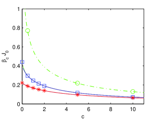
In order to compare the predictions based on Eq. (33) we measured by direct simulation the location of the critical points for several values of the average connectivity, $c=0,0.5,1,1.5,2,5$ and $10$ and the results, for each spatial dimension, are plotted in Fig. 1. The average over disorder was done by considering averages over 10 samples.

Table 1: (Color online) Results of Binder cumulant crossings for $d_{0}=2$ and $J_{0}>0$. In the column $\beta_{L,L^{\prime}}J_{0}$ we list the crossing inverse temperatures between the cumulants for systems of side $L$ with $L^{\prime}=128$. In the column $\beta_{c}J_{0}$ we list the critical parameters obtained from Eq. (33). The crossing values of the cumulant are listed in the column $U^{*}_{L,L^{\prime}}$.

$c$	$L$	$\beta_{L,L^{\prime}}J_{0}$	$\beta_{c}J_{0}$	$U^{*}_{L,128}$
	16	0.4410		0.612
0	32	0.4409	$0.440686...$	0.612
	64	0.4411		0.615
	16	0.2968		0.33
0.5	32	0.2964	0.2963	0.30
	64	0.2960		0.27
	16	0.2466		0.32
1.0	32	0.2461	0.2461	0.28
	64	0.2460		0.28
	16	0.2139		0.30
1.5	32	0.2137	0.2134	0.29
	64	0.2136		0.28
	16	0.1894		0.30
2.0	32	0.1891	0.1897	0.27
	64	0.1888		0.24
	16	0.1173		0.28
5.0	32	0.1174	0.1167	0.29
	64	0.1173		0.27
	16	0.0730		0.28
10.0	32	0.0730	0.0728	0.28
	64	0.0731		0.30

For the case $d_{0}=2$ we present in Table 1 detailed numerical results. For the cumulant crossing $\beta_{L,L^{\prime}}J_{0}$ (third column) listed for several values of $c$ we estimate a statistical error $0.0005$ which allows us to claim a good agreement between the simulations and the theoretical prediction obtained from Eq. (33) (fourth column). The values of the cumulant at the critical point for the pure model ($c=0$) are close to the value $0.61069$ calculated in CumulantIsing . The long-range links introduced by the disorder change the universality class from 2d Ising to mean-field.

The mean-field value of the Binder cumulant at criticality for an infinite system is predicted to be $0.2705$Luijten1995 ; Parisi2 ; Luijten1999 which is close to our estimates of Binder cumulant intersections listed in table 1 (fifth column) for which we estimate an error equal to $0.02$. In three dimensions we simulated only systems of side $L=8$ and 16. For $c=0$ the two cumulants intersect at the value $U_{L}=0.486$ close to the estimation $0.46521$ reported in Ising3d . For the other values of $c$ studied, $c=0.5,1,1.5,2,5$ and $10$ the intersection was measured near $U_{L}=0.31$. In one dimension we studied only $c=0.5,5$ and $c=10$ and also the Binder cumulant intersections were found to be near $0.3$ for intersections of $L=128,256,512,1024$ with $L^{\prime}=2048$.

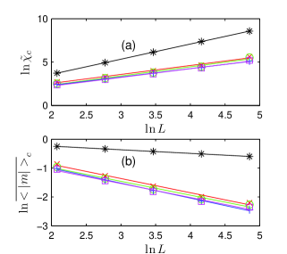
Furthermore, for $d_{0}=2$, we measured the scaling with system size of the average value of the absolute value of the magnetization $\overline{\left<|m|\right>}(\beta_{c}J_{0})$ and the susceptibility, $\tilde{\chi}(\beta_{c}J_{0})$ at the critical point. For a mean-field universality class these quantities are expected to scale at criticality like $\overline{\left<|m|\right>_{c}}\sim N^{-1/4}\sim L^{-d_{0}/4}$ and $\tilde{\chi}_{c}\sim N^{1/2}\sim L^{d_{0}/2}$ where $N$ is the total number of spins Luijten1995 ; Parisi2 ; Luijten1999 . In Fig. 2 we show these quantities plotted in bi-logarithmic scale as a function of system size for the different $c$ values studied. For the magnetization, the slope of the straight line fit for $c=0$ is $-0.125(1)$ and for the susceptibility is $1.752(1)$, consistent with the known exact exponents of the pure $d_{0}$=2 Ising model. For $c=0.5,1,1.5$ and $2$ we got, respectively, for the magnetization exponents $-0.49(3),-0.48(3),-0.52(2)$ and $-0.48(3)$ close to the expected value $-0.5$; whereas for the susceptibility we obtain the exponents $1.03(5),1.06(7),0.97(2)$ and $1.01(5)$, also close to the expected result for mean-field behavior.

Figure 2: (Color online) In (a) we plot the susceptibility, $\tilde{\chi}_{c}$, and in (b) the magnetization, $\overline{\left<|m|\right>}_{c}$, at the critical point for the $d_{0}=2$ model with $J/J_{0}=1$ as a function of the system side $L$. Both in (a) and (b) the data are for $c=0(\star),0.5(\times),1(\bigcirc),1.5(+),2(\square)$.

IV.2 Correlation functions above the critical temperature

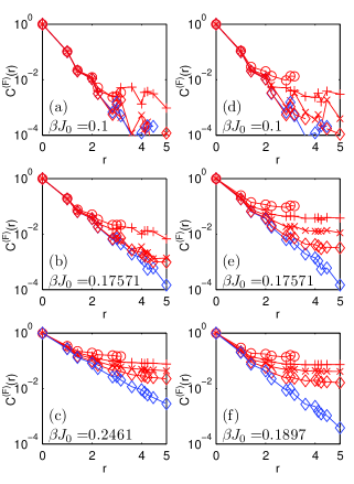
From Eq. (24) we see that the effective field theory, in the P region and zero external field, predicts the spin-spin correlation function of the random model $C^{(F)}$ to be, in the thermodynamic limit, equal to the correlation function of the pure model calculated at the same temperature. In order to check this result we calculated, from simulation,

$$C^{(F)}(r)=\overline{\left<\sigma_{0}\sigma_{r}\right>},$$ (37)

where $\sigma_{0}$ is an arbitrary spin and $\sigma_{r}$ is one spin at Euclidean distance $r$ from the spin $\sigma_{0}$, measured on the lattice $\mathcal{L}_{0}$. We considered the case $d_{0}=2$ with $J=J_{0}$ and $c=1$ and $2$ and the inverse temperatures $\beta J_{0}=0.1,0.17571$. These temperatures are above the critical temperatures for the two values of $c$ studied. We studied also the correlation function at the critical inverse temperatures $\beta_{c}J_{0}=0.2461$ and $\beta_{c}J_{0}=0.1897$ for $c=1$ and $c=2$, respectively (see Table 1). These calculations were done for system sides $L=8,16,32$ and $64$. In Fig. 3 we can see that, as the system size increases, the curves $C^{F}(r)$, for $c>0$, approach the data points for $c=0$ calculated for a system of size $L=64$. Note that, as we approach the critical temperature, the correlation function at large $r$ reaches a finite value that decreases as the system size increases. This finite constant is just due to the finite size of the system and it is predicted by the theory to vanish as $1/N$, in the thermodynamic limit, but at the same time it is responsible for the divergence, with system size, of the susceptibility at the critical point (see Eq. (33) and subsequent comments of Ref. SW ).

Figure 3: (Color online) Correlation functions $C^{(F)}(r)$ as a function of Euclidean distance $r$ for $J=J_{0}$ and $c=1$ (in (a), (b) and (c)) and $c=2$ (in (d), (e) and (f)) at different temperatures, $\beta J_{0}=0.1$ ((a) and (d)), $0.17571$ ( (b) and (e)). In (c) with $\beta_{c}J_{0}=0.2461$ and in (f) with $\beta_{c}J_{0}=0.1897$ (the critical temperatures for $c=1$ and $c=2$, respectively). The lower line (which is blue in the online version of this paper) is $C^{(F)}(r)$ for the pure model $c=0$ and for a system side $L=64$ ($\Diamond$). Data for four system sides are plotted, $L=8$ ($\bigcirc$), $L=16$ ($+$), $L=32$ ($\times$), $L=64$ ($\Diamond$).

IV.3 Susceptibility and Magnetization at non-zero external field above the critical temperature

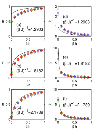
In the P phase at zero external magnetic field the effective field theory prediction for the susceptibility is exact, consistently with the exact predictions for the critical temperatures. The question remains whether the susceptibility prediction is a good approximation for non-zero field. To verify this we made simulations for the case $J_{0}=0$ with a positive long-range coupling (as in Eq. (10)) (in other words the simplest version of Viana-Bray model). For this particular case the magnetization is predicted to be given by the solution of the following equation

$$m=\tanh\left(c~{}m~{}\tanh(\beta J)+\beta h\right)$$ (38)

and the susceptibility (divided by $\beta$) is given by,

$$\tilde{\chi}(\beta J,\beta h)=\frac{1-m^{2}}{1-c(1-m^{2})\tanh\beta J}$$ (39)

In Fig. 4 we compare the results of the above predictions for the magnetization and susceptibility with simulation results for $c=2$. For averaging purposes we considered $10$ samples. The plots correspond to three temperatures $(\beta J)^{-1}=1.2903$ (first row), $(\beta J)^{-1}=1.8182$ (middle) and $(\beta J)^{-1}=2.1739$ (bottom). The critical temperature is $(\beta_{c}J)^{-1}=1.8205$. By construction, in the limit of strong field the magnetization prediction becomes exact and similarly in the limit of small field above the critical temperature. In the intermediate field range we see that the magnetization prediction and simulation results in general do not agree. However, above the critical temperature, the susceptibility obtained from simulation and the theoretical prediction given by Eq. (39) are very close to each other over the full range of field values studied. Note that for $(\beta J)^{-1}=1.8182$, close to the critical temperature, the simulation susceptibility shows, as expected, a strong finite-size effect at zero field.

It is worth to observe that with respect to our effective field theory, the Viana-Bray model represents the worst, i.e., the most difficult, case. The theory in fact, by construction, takes exactly into account all the effects due to the short-range couplings and to the short-loops present in the given lattice $\mathcal{L}_{0}$, and the greater is $d_{0}$, the greater is the level of accuracy of the theory also out of the P region (at least in the absence of frustration), while in the Viana-Bray model topologically we have $d_{0}=0$.

Figure 4: (Color online) Magnetization ( (a), (b) and (c) ) and Susceptibility ( (d), (e), (f)) for the Viana-Bray model and $c=2$ for three temperatures as a function of the external magnetic field. The lines are the theoretical predictions ( see Eqs. (38) and (39)) and the data points are simulation results for $N=128(.),256(\circ),512(+),1024(\times)$ and $2048(\Diamond)$. For the case studied here the critical temperature is, $(\beta_{c}J)^{-1}=1.8205$.

IV.4 Negative short-range coupling and second order phase transitions

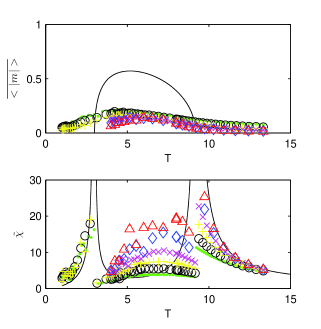
In the case $J_{0}<0$ the theory allows for the occurrence of two second-order phase transitions. At low and high temperatures the system is disordered and in the intermediate temperatures a ferromagnetic phase arises. The simulations confirm this phase diagram picture. We made simulations at $d_{0}=1$, for $J_{0}=-0.5$, $J/J_{0}=-20$ and $c=1.4$. We made averages over disorder by considering 50 samples and we studied system sizes $L=512,1024,2048,4096,8192$ and $16384$. In Fig, 5 we plot the magnetization and the susceptibility as a function of temperature, $T$. The two critical points are predicted to occur at $T_{c,1}=2.985$ and $T_{c,2}=9.207$. The predicted values of the magnetization in the intermediate temperature range, $T_{c,1}<T<T_{c,2}$, are different from the simulation results (see Fig. 5). However, the theoretical predicted susceptibility, in both P phases, is very close to the simulation susceptibility approaching each other as the system size increases.

Note that this model is a frustrated system so that large fluctuations and strong finite size effects are present, especially close to the lower temperature critical point where we do not perform high precision simulation as it requires averaging over a large number of samples. We have studied, in detail, the high temperature critical point where we applied the cumulant crossing technique.

Figure 5: (Color online) Magnetization (top) and susceptibility (bottom) as a function of temperature for a $d_{0}=1$ system with $J_{0}<0$. The average connectivity is $c=1.4$ and $J_{0}=-0.5$, $J/J_{0}=-20$. The line is the theoretical prediction and the data points correspond to different system sizes, $L=512(.),1024(\circ),2048(+),4096(\times),8192(\diamond),16384(\triangle)$.

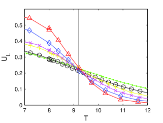
The intersection temperatures of the cumulants for $L=512,1024,2048,4096$ with the system of size $L=16384$ were, $9.24,9.35,9.23,9.32$, respectively, from which we can estimate a critical temperature equal to $9.29(6)$. This estimate is close but slightly higher than the predicted critical temperature, $T_{c,2}=9.207$. However, considering the statistical error and the finite size corrections we cannot exclude a convergence toward the theoretical value in the thermodynamic limit. The corresponding intersection values of the cumulant were, $0.23,0.21,0.23,0.21$. These values are smaller than the values in the range $0.27-0.3$ that we measured in section IV.1 for $J_{0}>0$. In the Fig. 6 we plot the Binder cumulant as a function of temperature for the system sizes studied.

Figure 6: (Color online) Binder cumulant $U_{L}$ as a function of temperature for a $d_{0}=1$ system with $J_{0}<0$. The average connectivity is $c=1.4$ and $J_{0}=-0.5$, $J/J_{0}=-20$. The vertical line is the theoretical prediction for the critical temperature and the data points correspond to different system sizes, $L=512(.),1024(\circ),2048(+),4096(\times),8192(\diamond),16384(\triangle)$.

IV.5 Negative short-range coupling, first-order and spin-glass phase transitions

We considered the case for $c=10$, $J_{0}=-0.9$ and $J=0.5$ at $d_{0}=1$. From the theory it turns out that for temperatures above $2.38$ only the zero magnetization solution is stable but for temperatures lower than this value there are always two stable solutions, one with non-zero magnetization and another with zero magnetization. For temperatures $T<2.34$ the nonzero magnetization solution has the lower free-energy so that a first-order phase transition is predicted at this temperature. The theory also predicts a possible spin-glass phase transition at a temperature, $T_{c,SG}=1.88$. Note that the theory always predicts continuous spin-glass phase transitions.

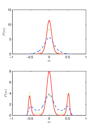
We made simulations for systems of size $L=512$, $1024$, $2048$, $4096$ and $8192$ and as before we neglected $10^{5}$ MCS/N for equilibration purposes and we made measurements for $10^{6}$ MCS/N. The averaging over disorder was made by considering 50 samples. The results show a first order phase transition occurring at slightly lower temperatures than the one predicted by the theory. The probability distribution of the magnetization clearly exhibits (see Fig. 7) the behavior characteristic of first-order phase transitions vollmayr1993 namely the emergence, at temperatures close to the transition, of two maximum located at symmetric nonzero values together with a third maximum near zero magnetization.

Figure 7: (Color online) Simulation results for the magnetization probability distribution, $P(m)$, for the model with $c=10$, $J_{0}=-0.9$ and $J=0.5$ at $d_{0}=1$. In (a) we plot curves for $L=8192$ (solid line), $L=4096$ (dotted line) at $T=2.05$ and $L=2048$ (dashed line) at $T=2$ and in (b) we plot the corresponding data for $L=8192$ and $L=4096$ at $T=1.86$ and $L=2048$ at $T=1.83$.

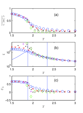
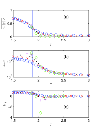
In Fig. 8(a) we show the simulation results for the average magnetization, the magnetic susceptibility (b), and the magnetization Binder cumulant (c). The simulation susceptibility follows very closely the zero magnetization theoretical susceptibility up to temperatures lower than the predicted $T_{c}$. Note that, in the case under study, the zero magnetization solution is a stable solution at any temperature and the theoretical prediction of the phase transition is based on comparison of the value of free-energies of the solutions. The theory does not predict correctly the location of the transition since values of the free-energy of the non-zero magnetization solution are not given exactly by the theory. The simulation Binder cumulant shows, near the transition temperature, the expected increasingly negative values, as the system size increases vollmayr1993 . Interestingly, the simulation data give a transition temperature close to the theoretically predicted spin-glass transition temperature.

We also studied the overlap order parameter distribution and the results are shown in Fig. 9. Here, also, the behavior expected for a first-order transition temperature was observed. The negative value minima of the Binder cumulant for the overlap order parameter are steeper and occur at slightly higher temperatures, for the same system sizes, as compared with the corresponding quantity for the magnetization.

Figure 8: (Color online) Simulation results for the average magnetization (a), magnetic susceptibility (b) and Binder cumulant $U_{L}$ (c) as a function of temperature for the model with $c=10$, $J_{0}=-0.9$ and $J=0.5$ at $d_{0}=1$. In (b) we have used $\tilde{\chi}=N\overline{<m^{2}>}$ at any temperature. The vertical lines are at $T_{c}=2.34$ and $T_{c,SG}=1.88$. In (b) the line is the theoretical susceptibility for the zero magnetization solution. The simulation data points are for $L=512(\bigcirc),1024(\times),2048(.),4096(+),8192(\diamond)$.

Figure 9: (Color online) Simulation results for the average overlap order parameter, $\overline{<|q|>}$ (a), $\tilde{\chi}_{SG}=N\overline{<q^{2}>}$ (b) and Binder cumulant, $U_{q}$ (c), as a function of temperature for the model with $c=10$, $J_{0}=-0.9$ and $J=0.5$ at $d_{0}=1$. The data points are simulations for $L=512(\bigcirc),1024(\times),2048(.),4096(+),8192(\diamond)$.

Quite interestingly for $c=4.5$ and the values of the coupling constants, $J_{0}=-0.9$ and $J=1$, the theory predicts the absence of ferromagnetic phase transitions and only a continuous P-SG phase transition located at $T_{c}^{(SG)}=2.29$.

Figure 10: (Color online) Results for the model with $c=4.5$, $J_{0}=-0.9$ and $J=1$ at $d_{0}=1$. In the top plot we show the temperature dependence of the Binder cumulant for the overlap order-parameter. The lines are fits made for each system size. The vertical line is the location of the predicted spin-glass critical temperature. The inset shows the average values of the overlap order parameter together with the effective field theory prediction for this quantity. In the bottom plot we show the temperature dependence of the magnetic susceptibility. The inset shows the average magnetization as a function of temperature. For all the plots the data points correspond to simulations for systems of sides, $L=512(\bigcirc),1024(\times),2048(.),4096(+)$.

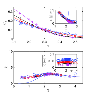
The obtained simulation results are shown in Fig. 10. The number of samples was 100 and the simulation times considered here were the same as for the case $c=10$. In the top plot we see that $U_{q,L}$ for different system sizes intersects very near the theoretically predicted critical temperature. The inset of the top plot shows the average overlap order parameter that decreases with system size above the spin-glass critical temperature. In the lower plot we see that the magnetic susceptibility is almost independent of system size and it agrees with the theoretical prediction for temperatures above the spin-glass phase transition while it deviates at lower temperatures.

IV.6 Bimodal Edwards-Anderson model

The bimodal Edwards-Anderson modeledwards is a disordered spin model where the nearest neighbor coupling $J_{0}$ of Ising type spins has the bimodal distribution in (12). Here, we consider the two dimensional square lattice version of the model with additional long-range couplings. The pure model (without long range shortcuts) is known to show a P-SG phase transition only at zero temperature being the lower critical dimension of the model equal to two Hartmann ; katzgraber .

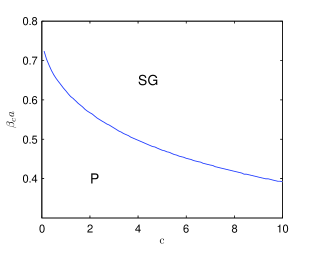
To apply the effective field theory, for each phase $\Sigma=$F or SG, we have to consider the pure Ising model magnetization (13) and susceptibility (30) calculated by using the definitions of the effective long- and short-range couplings $J^{(\Sigma)}$ and $J_{0}^{(\Sigma)}$, from Eqs. (14)-(23), respectively. By using the numerical two-dimensional Ising model magnetic susceptibility, we can obtain the expected location of the spin-glass phase transition. The result of this calculation is shown in Fig. 11. We stress that theory predicts that the inclusion of an arbitrary small number of long-range shortcuts in the Edwards-Anderson model leads always to a finite temperature phase transition. In fact, in the limit of an infinitesimal addition of short-cuts, the theory predicts a P-SG transition at the finite value given by $\beta_{c}\,a=\tanh^{-1}[\sqrt{\tanh(0.44068...)}]=0.7642...$,where $0.44068...$ is the critical inverse temperature of the regular two-dimensional Ising model with a unitary positive coupling. This implies that the EA model with short-cuts, in the limit $c\to 0^{+}$, is not equivalent to the original EA model without short-cuts. In other words, the EA model is not thermodynamically stable under graph noise.

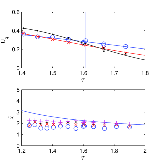
We made simulations for the EA model with $a=1$, $J=1$ and $c=1$ to compare with the predictions of the theory. The average over disorder was done by considering 100 samples. We neglected the first $10^{5}$ MCS/N for equilibration and made measurements for $10^{6}$ MCS/N. For $c=1$ the expected critical temperature is $T_{c}^{(SG)}=1.6057$. In Fig. 12 (top panel) we obtained crossings of the overlap parameter Binder cumulant for system sizes $L=8,16$ and $32$. The statistical error of the Binder cumulant, as expected, increases with system size and we excluded from the Binder cumulant intersection calculations the data for $L=64$. Our numerical estimate of the critical temperature is $T_{c}^{(SG)}=1.6(1)$ still consistent with the expected critical temperature.

Since, for an Ising model with zero coupling and zero external magnetic field $\tilde{\chi}_{0}=1$, the prediction for the magnetization and the magnetic susceptibility is $<|m|>=0$ and $\tilde{\chi}=[1-c\tanh(\beta J)]^{-1}$. In Fig. 12 (lower panel) we plot the magnetic susceptibility simulation results together with this theoretical prediction. We see that in the P phase the numerical estimates of the susceptibility approach the theoretical curve as the system size increases.

Figure 11: (Color online) Phase diagram for the $d_{0}=2$ Edwards-Anderson model with long-range connections and coupling constant $J=1$ . The curve is the value of $\beta_{c}a$ for the SG phase transition as obtained from equation (32) and our numerical results for the pure Ising model susceptibility for a system of side $L=128$.

Figure 12: (Color online) Results for the $d_{0}=2$ Edwards-Anderson model with long-range connections with $a=J=1$ at $c=1$. The top plot shows values of the Binder cumulant as a function of temperature and the bottom plot shows the temperature dependence of the magnetic susceptibility. The simulations were done for $L=8$ ($\bigcirc$), $L=16$ ($\times$), $L=32$ (.) and $L=64$ ($+$). In the top plot the vertical line is the theoretical prediction of the spin-glass critical temperature and the lines are polynomial fits of the Binder cumulants for each system size. In the lower plot the line is the theoretical prediction for the magnetic susceptibility.

V Conclusions

In this work we have compared the predictions of an effective field theory for several Ising models on small world networks with Monte Carlo simulation results. All the predictions of the theory, where it is known to be exact, namely in the P region at zero external field, were confirmed by the simulation results. In particular we have checked the critical surfaces $(T,c)$, the temperature dependence of the susceptibility, and the spin-spin correlation function.

Furthermore, for the simplest version of the model, i.e., the Viana-Bray model (where $d_{0}=0$), we studied the effect of a non-zero external field. Although the theory is not exact in this case, there is a reasonable agreement between the predicted field dependence of the magnetization and susceptibility specially above the critical temperature. For the case of $J/J_{0}=-20$ and $c=1.4$ at $d_{0}=1$ we verified the existence of two second order phase transitions. A good agreement between the theoretical temperature dependence of the susceptibility in the P phases and simulation results was observed. The location of the high temperature critical point was explicitly verified using the cumulant crossing technique.

For a one-dimensional model with $J_{0}=-0.9$, $J=0.5$ and $c=10$, we observed a first order phase transition as predicted by the theory but at a lower temperature. This may be a consequence of the fact that in this case, unlike the second-order phase transitions cases, the zero magnetization solution does not become unstable at the transition temperature and - consistently with the fact that the theory does not give exact results out of the pure P regions - the critical point obtained as the point where the two free-energy values equal is not exactly predicted. Quite interestingly, we find that also the P-SG phase transition turns out to be first-order and, furthermore, its critical point seems to coincide with the theoretical one.

With the couplings $J_{0}=-0.9$, $J=1$ and a smaller average connectivity, $c=4.5$ the theory predicts that only a P-SG transition is present. We studied by simulation this spin-glass critical behavior and we found the critical temperature very close to the theoretical prediction.

We also introduced a model not previously studied, the two dimensional Edwards-Anderson model with added long-range shortcuts, where we confirmed that even an infinitesimal inclusion of shortcuts makes the spin-glass phase transition to occur at a finite non-zero temperature. In other words, as the theory predicts, we find that the two dimensional Edwards-Anderson model is not thermodynamically stable under graph-noise.

The class of disordered models for which the theory is applicable is very wide and its application just relies on the availability of numerical or analytical results for the susceptibility of non disordered models in arbitrary $d_{0}$ dimensions. When there is strong frustration, simulations are difficult to perform requiring large simulation times and averages over many samples. Our results clearly confirm the usefulness of the effective field theory proposed in SW by giving accurate predictions for the models phase diagram. The possibility to improve the theory out of the P region opens a new interesting challenge.