The QUaD Galactic Plane Survey 1: Maps And Analysis of Diffuse Emission

Abstract

We present a survey of $\sim 800$ square degrees of the galactic plane observed with the QUaD telescope. The primary product of the survey are maps of Stokes I, Q and U parameters at 100 and 150 GHz, with spatial resolution 5 and 3.5 arcminutes respectively. Two regions are covered, spanning approximately $245-295^{\circ}$ and $315-5^{\circ}$ in galactic longitude $l$, and $-4<b<+4^{\circ}$ in galactic latitude $b$. At $0.02^{\circ}$ square pixel size, the median sensitivity is 74 and 107 kJy/sr at 100 GHz and 150 GHz respectively in I, and 98 and 120 kJy/sr for Q and U. In total intensity, we find an average spectral index of $\alpha=2.35\pm 0.01\mathrm{(stat)}\pm 0.02\mathrm{(sys)}$ for $|b|\leq 1^{\circ}$, indicative of emission components other than thermal dust. A comparison to published dust, synchrotron and free-free models implies an excess of emission in the 100 GHz QUaD band, while better agreement is found at 150 GHz. A smaller excess is observed when comparing QUaD 100 GHz data to WMAP 5-year W band; in this case the excess is likely due to the wider bandwidth of QUaD. Combining the QUaD and WMAP data, a two-component spectral fit to the inner galactic plane ($|b|\leq 1^{\circ}$) yields mean spectral indices of $\alpha_{s}=-0.32\pm 0.03$ and $\alpha_{d}=2.84\pm 0.03$; the former is interpreted as a combination of the spectral indices of synchrotron, free-free and dust, while the second is attributed largely to the thermal dust continuum. In the same galactic latitude range, the polarization data show a high degree of alignment perpendicular to the expected galactic magnetic field direction, and exhibit mean polarization fraction $1.38\pm 0.08\mathrm{(stat)}\pm 0.1\mathrm{(sys)}$% at 100 GHz and $1.70\pm 0.06\mathrm{(stat)}\pm 0.1\mathrm{(sys)}$% at 150 GHz. We find agreement in polarization fraction between QUaD 100 GHz  and WMAP W band, the latter giving $1.1\pm 0.4$%.

1. Introduction

Radio and sub-mm observations of the galactic plane yield important insights into many astrophysical processes associated with galaxies like our own, from the large scale properties of magnetic fields, to smaller scale phenomena associated with star formation.

These properties can often be inferred from low resolution observations of diffuse galactic components, or large samples of representative objects distributed through the galaxy. Three mechanisms contribute to the diffuse galactic emission in total intensity in the radio and sub-mm: Synchrotron radiation, which dominates below $\sim 60~{}\mathrm{GHz}$ and is caused by relativistic electrons spiralling in magnetic fields; free-free emission, which is generated by non-relativistic electron-ion interactions; and radiation from vibrational modes of thermal dust, whose emission dominates above $\sim 100~{}\mathrm{GHz}$. Of these, synchrotron and dust are appreciably polarized, with typical polarization fractions close to the galactic plane of $\sim 2-4\%$ and $\sim 1\%$ respectively (Kogut et al., 2007); both result in polarized light aligned perpendicular to the magnetic field.

The polarization of dust is due to prolate grains aligning with their long axis perpendicular to the local magnetic field (Lazarian, 2003), with the polarization fraction dependent on the grain size distribution and their overall alignment (e.g. Prunet et al., 1998). Observations of polarized starlight via dust absorption have indirectly demonstrated a large degree of coherence of the magnetic field in our galaxy and others (Heiles, 1996; Zweibel & Heiles, 1997). However, these measurements can be biased by lines of sight with low column densities (Benoît et al., 2004) and therefore more direct probes of the galactic dust are desirable, not only for the study of dust in its own right, but as a probe of the magnetic field responsible for most large-scale polarized emission in the galaxy (e.g. Hildebrand et al., 2000). Sub-mm polarization vectors can be reasonable tracers of the magnetic field structure even for relatively dense clouds, and are therefore an attractive option for this line of study.

The emissive properties of dust in the sub-mm have also attracted attention from the CMB community, since diffuse galactic polarization poses a challenging obstacle to the detection of primordial gravitational waves via the ‘B-mode’ polarization signal (e.g. Hu & White, 1997; Dunkley et al., 2009). As the B-mode power spectrum is predicted to peak on angular scales $\sim 1^{\circ}$, characterization of dust as a foreground is essential to account for this ‘contaminant’ from surveys over large areas of sky, such as that expected from the Planck satellite (Villa et al., 2002).

Observational constraints on diffuse galactic polarization from dust are currently limited to a small number of experiments, including WMAP from $23$–$94$ GHz at resolution up to $\sim 0.25^{\circ}$ (Kogut et al., 2007; Gold et al., 2009), and Archeops at $353$ GHz smoothed to $\sim 1^{\circ}$ resolution (Benoît et al., 2004; Ponthieu et al., 2005). While a variety of models exist for estimating the unpolarized contribution of dust (e.g. Finkbeiner et al., 1999, hereafter FDS), the limited number of experiments at dust-dominated frequencies has prevented detailed comparison to observations. Furthermore, the lack of angular resolution of such experiments means emission from diffuse and discrete sources cannot be separated, particularly in the plane of the galaxy ($|b|<10^{\circ}$).

The study of discrete sources at and above $100$ GHz yields insights into the process of star formation. In star forming regions, thermal dust efficiently absorbs UV light from star formation, and re-radiates in the sub-mm where dust is optically thin. Observations near the spectral peak can therefore probe the centers of dense cores and constrain the stellar core mass function (e.g. Netterfield et al., 2009; Schuller et al., 2009; Olmi et al., 2009).

In this paper we report an $\sim 800$ square degree survey of the galactic plane with the QUaD telescope, which operated at 100 and 150 GHz with angular resolution of $5^{\prime}$ and $3.5^{\prime}$ respectively, in Stokes I, Q and U parameters. A survey of this size, frequency and angular resolution can be used to investigate the polarized and unpolarized properties of both diffuse emission and discrete sources. The mapmaking and properties of the diffuse emission form the core of this paper; a companion publication (hereafter the “Source Paper” — Culverhouse et al. in prep.) contains analysis of the compact source distribution in the survey.

2. Instrument Summary and Observations

Here we summarize the features of the QUaD experiment — a detailed description can be found in (Hinderks et al., 2009), hereafter referred to as the “Instrument Paper”. QUaD was a 2.6 m Cassegrain radio telescope on the mount originally constructed for the DASI experiment (Leitch et al., 2002), and enclosed in an extended reflective ground shield. The receiver consisted of 31 pairs of polarization sensitive bolometers or PSBs (Jones et al., 2003), 12 at 100 GHz, and 19 at 150 GHz, with each PSB pair located within a single feed. The PSB pairs were split into two orientation groups to allow simultaneous measurement of Stokes Q and U. QUaD operated from February 2005 to November 2007; the observations reported in this paper were taken over 40 days between July and October 2007.

As with the QUaD CMB observations (Ade et al., 2008; Pryke et al., 2009; Brown et al., 2009), the second of which we refer to as “P09”, a lead-trail field differencing scheme was employed to allow subtraction of contaminating ground pickup. Each day, nine lead-trail pairs of fields were observed, with the lead field tracking center aligned with the plane of the galaxy $b=0$. For each lead field, the companion trail field repeated exactly the same azimuth (az) and elevation (el) scan pattern with respect to the ground, but with the tracking center 1hr later in RA. In order to minimize the possibility of temporal variation in ground signal, each trail field was observed immediately after its companion lead field, resulting in a lead 1, trail 1, lead 2, trail 2 etc ordering — see Figure 1 for a plot of this scheme. Though the signal levels in trail fields are generally much smaller than the lead field, some spurious signal is introduced into the lead field due to field-differencing. A discussion of this effect is presented in Appendix A.3, while Appendices B.1 and B.2 demonstrate that the recovery of global parameters of the diffuse emission are unaffected by field-differencing or filtering.

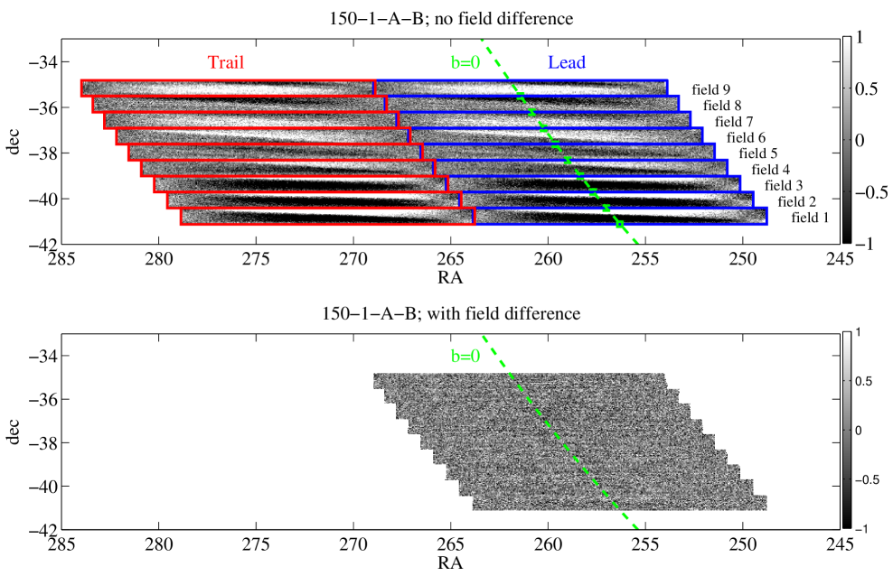
Figure 1.— Top: Coadded PSB pair difference map of a single 150 GHz  feed from one day of observations, with no field difference. The nine rectangular lead-trail pairs of fields observed on this day are shown in blue and red respectively. Note the strongly polarized ground pickup which repeats between lead-trail pairs. The colour scale is MJy/sr, with the green line indicating the plane of the galaxy. Green squares indicate the starting point of the scan pattern for each field. Bottom: As above, but with field differencing applied — the ground signal is now heavily suppressed.

Whilst tracking each field center, the telescope scanned forward and backward in az with a total az range of 15^∘ at a rate of 0.4^∘/s, followed by a step of -0.02^∘ in elevation. This was repeated 35 times to build up a raster map of the sky, before slewing to the next field where the same scanning pattern was repeated. Each field took approximately 1hr observing time, and covered 0.7^∘ in dec, a total of 6.3^∘ per day. Figure 1 shows a graphic representation of the scanning strategy, and demonstrates that ground signal is cleanly removed by field-differencing.

The entire survey coverage is shown in Figure 2, and was limited in declination range by two factors. First, the beams intersect the ground shield at elevations lower than $\sim 25^{\circ}$ ($\mathrm{dec}>-25^{\circ}$). Second, at $\mathrm{dec}<-60^{\circ}$ the galactic plane is nearly parallel to the horizon — filtering the scans, necessary to remove atmospheric contamination, would remove the bulk of the diffuse galactic emission unless the scan length was massively increased, resulting in a loss of sensitivity.

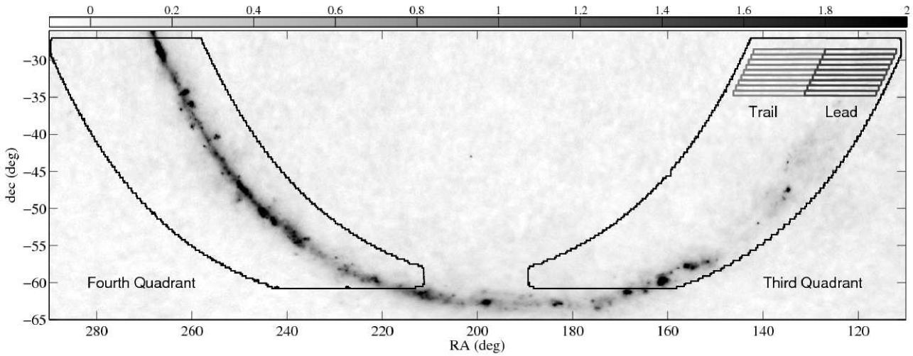
Figure 2.— Total QUaD galactic survey area at 150 GHz (black lines) plotted over WMAP 5yr W band total intensity map (Hinshaw et al., 2009). The color scale is in MJy/sr. For one day of data, lead field coordinates for center pixel are plotted in dark gray; trail fields are in light gray. This lead-trail observing strategy is repeated over the rest of the survey region within the black locus.

Two portions of the galaxy are available between $-60$ and $-25^{\circ}$ in dec, between $110^{\circ}<\mathrm{RA}<190^{\circ}$ and $210^{\circ}<\mathrm{RA}<290^{\circ}$. In galactic longitude and latitude ($l$,$b$) these correspond to a latitude range approximately $-4^{\circ}<b<4^{\circ}$, and $240^{\circ}<l<295^{\circ}$ and $315^{\circ}<l<5^{\circ}$ — hereafter, these two regions are loosely termed the ‘third quadrant’ and ‘fourth quadrant’. With our coordinate constraints, the third and fouth quadrant regions each spanned $32^{\circ}$ in dec; the 40 days of observations were equally divided between the two regions, allowing four complete passes over each.

3. Low Level Data Processing

Low-level processing of the raw timestream is performed using the same steps described in P09. The timestream is deconvolved to remove the effect of the bolometer timeconstants, deglitched, and downsampled. Between observations of each field, relative gains between PSB pairs in a feed, and between feeds in each frequency group, are determined using ‘el-nods’. In this calibration procedure, the telescope is moved first up then down by one degree in elevation — this injects a large signal into the timestream due to the common-mode atmospheric gradient; further details are given in the Instrument Paper.

As seen in Figure 1, the ground pickup is strong compared to the sky signal of interest. A misalignment between absolute lead and trail field azimuth coordinates $\delta\mathrm{az}$ causes ground signal to cancel imperfectly, and can lead to significant contamination for $\delta\mathrm{az}>0.1^{\circ}$. This is carefully corrected by using the pointing information to realign the lead and trail fields on a scan-by-scan basis, at the expense of a small quantity of data where there is no overlap between lead and trail scans. Approximately one out of nine lead-trail pairs require correction of up to $0.4^{\circ}$, leading to a loss of data of order 0.1%.

Further data is rejected from visual inspection of field-differenced maps, made using sum and difference data from each feed. Maps of the same fields taken on different days are compared to distinguish the repeatable sky signal from spurious contamination. The pair difference maps in particular are useful because the amplitude of the contamination, which appears as spurious $1/f$ noise, is considerably larger than that of the polarized galactic signal. Typical rejection rates are one out of nine fields for four bolometer pairs, a loss of data of $\sim 0.75\%$.

4. Mapmaking

The map-making scheme used here is a multi-stage adaptation of the ‘naive’ mapping used in P09, and requires information on telescope pointing (both absolute and the relative offsets of each PSB in the focal plane), and the PSB angles and efficiencies to construct the Stokes I, Q and U maps. As in P09 and unless stated otherwise, the pixelization for all maps in this paper is in RA and dec, using 0.02^∘ square pixels. Further details of constructing I, Q and U maps from timestream may be found in P09; here we summarize the basic points.

4.1. Pointing, PSB Angles and Efficiencies

Absolute pointing was determined from a nine parameter online pointing model, derived from optical and radio observations as described in the Instrument Paper. This was shown to have an absolute accuracy over the hemisphere of $\sim 0.5^{\prime}$ rms from pointing checks on RCW38 and other galactic sources, taken over two seasons of CMB observations.

The scatter in the centroid positions for a given detector relative to the boresight was consistent with the overall pointing wander of $\sim 0.5^{\prime}$ rms, and the offset angles of each detector around the focal plane showed no evidence for systematic changes with time. The detector offset angles used in mapmaking are the mean of the values observed from RCW38, with an estimated uncertainty of $\sim 0.15^{\prime}$.

PSB polarization angles and efficiencies were determined using a chopped thermal source placed behind a polarizing grid and observed at many angles — further details are given in P09 and the Instrument Paper. From these observations we also measure our mean cross polar leakage (the response of a single PSB to anti-aligned radiation) as $\epsilon=0.08\pm 0.015$. This mean value is applied to all channels when constructing maps, and all simulations include the scatter about the mean.

For an experiment of this type cross polar leakage does not imply leakage from total to polarized intensity — it is simply a small loss of efficiency, which is corrected by an additional calibration factor applied to the polarization data.

4.2. Mapmaking Algorithm

Before binning into maps, the data is first field-differenced to remove ground contamination — this operation is performed directly in the timestream. For each feed the sum and difference of the data is then taken for each pair of PSBs. To construct the I maps, we coadd the pair-sum data for each feed on each day. For polarization, a $2\times 2$ matrix inversion is required for each map pixel to convert from the pair difference data to Q and U maps. This matrix expresses the polarized sky intensity projected onto each PSB, which is measured in the pair-difference timestream. To invert such a matrix we require each pixel be measured at two PSB angles — this is achieved with the two orientation groups in the QUaD focal plane. However, before coadding the data into maps, timestream filtering is required to reduce the low-frequency noise, which causes striping in the scan direction in the maps.

4.2.1 Initial Filtering

In addition to detector noise, bolometer drifts and atmospheric $1/f$ noise are a large contribution to the sum data (since the atmosphere is largely unpolarized, its contribution is common-mode and is thus heavily suppressed in the difference data). The CMB analysis of P09 subtract a third-order polynomial from the timestream to limit the effects of this $1/f$ noise; though this filtering removes sky signal, the effect is accounted for in simulations, which is a feasible method for a power spectrum analysis. However, we are interested in the spatial distribution of the galactic signal, and the timestream may not simply be filtered in the same way. For example, in the sum data the bright galactic emission will dominate the polynomial fit, leading to regions of unphysical negative signal when the polynomial is subtracted from the data; a minimal level of filtering is therefore desirable. Here, the end portions of each scan — the most distant parts of the scan from the galactic plane — are used to determine a DC level and slope, which is then subtracted over the entire scan. The same procedure is used for total and polarized intensity data. This choice of filtering scheme effectively forces the maps to be zero at the edges, a consequence of our inability to measure the DC level of the sky brightness.

The amount of scan ends used is a trade off between better determination of the $1/f$ noise, which requires an increasing fraction of the scan, and larger regions of negative intensity in the final maps. The second of these effects arises because the DC level subtracted from the timestream is influenced more by the bright galactic signal as more of the scan is used.

After some experimentation, using a scan fraction $f_{s}=25\%$ (i.e. $\sim 12.5\%$ at either end) was found to result in total intensity maps with few negative regions, while keeping residual $1/f$ noise to a minimum. The quantitative results on the diffuse emission, presented in Section 5, are not significantly changed by adopting a different fraction of the scan, or using a mask of fixed width either side of the galactic plane.

From the sum/difference data we construct a minimally-filtered map, termed the ‘initial map’ or $m_{0}$: scans are filtered by removing a DC-level and linear slope, as described above. The timestream is then coadded into the map using the pointing information for each pair of PSBs, and weighted by the inverse scan variance as determined from the scan end data after filtering. A section of the $m_{0}$ survey map is shown in the top panel of Figure 3. Scan variances are coadded into a ‘variance map’, which produces an estimate of the pixel variance over the survey area.

4.2.2 Secondary Filtering

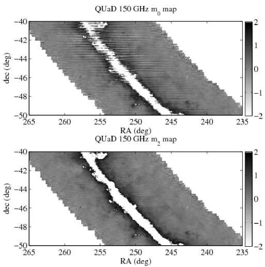
Figure 3.— Maps illustrating the destriping process on QUaD 150 GHz  data. All color scales are in MJy/sr, with saturated pixels within the survey region shown in white. Top: DC + slope filtered ($m_{0}$) map. Bottom: Destriped map $m_{2}$.

Small-scale noise between rows of map pixels (visible in the top panel of Figure 3) is further reduced by a destriping algorithm as follows. After the $m_{0}$ map is constructed, compact sources are located using the source extraction code described in the Source Paper, which is based on the SExtractor routine (Bertin & Arnouts, 1996). A second map ($m_{1}$) is generated identically to $m_{0}$, with the exception that sources located in the scan ends are masked during filtering. This process prevents discrete sources lying far from the bulk of the diffuse emission from influencing the inital polynomial filtering.

The simple removal of a DC-level and slope from each scan produces a map which still exhibits striping due to atmospheric $1/f$ noise. To suppress this noise, we construct a template for the sky signal, which is simply a smoothed version of the $m_{1}$ map. This template is then subtracted from the raw timestream, leaving data which is dominated by atmospheric noise. A 6th-order polynomial is then fit to the signal-subtracted timestream, and then subtracted from the original data. The timestream still contains the galactic signal of interest, but with the $1/f$ noise much suppressed compared to the simple DC+slope filtering described above.

Maps made with the secondary-filtered data are termed the $m_{2}$ maps — these exhibit improved noise properties without a heavy penalty in signal loss, as may be seen in Figure 3. A detailed discussion of the algorithm and its implementation is presented in Appendix A.

4.3. Absolute Calibration

Absolute calibration is applied using conversion factors from Brown et al. (2009). The maps used in the QUaD CMB analysis were cross-calibrated with the Boomerang experiment (Masi et al., 2006) to produce factors which convert from detector units of volts to thermodynamic units of $\mu$K. These are estimated to be uncertain at the 3.5% level. The galactic maps are calibrated using the same conversion factors, and then rescaled to brightness units using

$$dI=(dB/dT)_{2.73}\times dT,$$ (1)

where $B$ is the Planck function, and $dT$ and $dI$ represent thermodynamic and brightness fluctuations respectively. Througout the analysis in this paper, the central frequencies $\nu_{0}$ of the QUaD bands are loosely referred to as 100 and 150 GHz. Assuming a spectrally flat source, numerical integration of the QUaD bandpass presented in the Instrument Paper results in central frequencies of 94.5 and 149.6 GHz.

4.4. Final Maps

Calibrated, destriped survey maps of Stokes $I$, $Q$, and $U$ are shown in Appendix C, Figures 19–21 in celestial coordinates (the native coordinate system for map processing) . The 100 GHz maps are hereafter referred to as $I_{100}$, $Q_{100}$, and $U_{100}$, and likewise at 150 GHz. All polarization maps follow the IAU convention, in which $+Q$ is parallel to N-S and $+U$ parallel to NE-SW (Hamaker & Bregman, 1996). Converting to galactic coordinates (galactic longitude $l$ and latitude $b$) results in the maps shown in Figure 5. Total intensity maps are transformed from the native celestial coordinates to galactic $l$ and $b$ by linear interpolation of the map pixel values between the respective coordinate grids calculated with standard astronomical software packages. For polarization, we compute the angles between unit (RA,dec) vectors in the ($l$,$b$) basis at each point in the map — these angles are then used to project the polarized intensity onto the ($l$,$b$) basis.

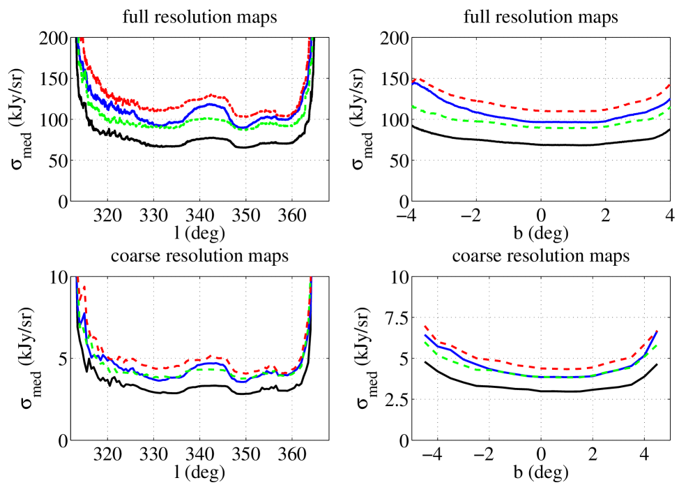
Figure 4.— Plots showing median sensitivity of the survey as a function of $l$ and $b$ for the fourth quadrant region data; plots for the third quadrant region are very similar. In all panels, black represents 100 GHz I, blue 150 GHz I, green 100 GHz Q, and red 150 GHz Q. The sensitivity to U is comparable to Q. Top row is for the full resolution (pixel size $0.02^{\circ}$) maps, while bottom row is for the coarse resolution ($0.5^{\circ}$ pixels) maps used for the analysis of diffuse structure in Section 5.

The median sensitivity of the survey as a function of $l$ and $b$ is plotted in Figure 4 for the fourth quadrant region, where the rms values are determined from the variance maps; the sensitivity is almost identical for the third quadrant. The QUaD galactic plane survey is fairly uniform over $\sim 50^{\circ}$ in $l$ and $|b|\leq 4^{\circ}$ in each region, allowing detection and characterization of diffuse and localized emission over $\sim 800$ square degrees of the low-latitude galaxy.

At the native map resolution of $0.02^{\circ}$, much of the diffuse emission and hundreds of compact sources are detected to high significance; particularly bright regions such as the galactic center reach signal-to-noise ratios $S/N>500$ in total intensity, with the bulk of the diffuse emission (within $\sim 3^{\circ}$ of the galactic plane) detected with $S/N>10$ per map pixel. In Figure 4 we also show the sensitivity for ‘coarse’ resolution maps with pixel size of $0.5^{\circ}$; in these maps, the equivalent brightness sensitivity is a factor $\sim 25$ higher than the full resolution maps. In polarization, there is significant diffuse polarized emission in the 150 GHz  fourth quadrant data at this resolution, while polarized signal at 100 GHz  becomes apparent when degrading to 0.5^∘ pixels. Note that when constructing coarse resolution maps, all timestream operations such as field-differencing, filtering and destriping are performed exactly as above. Locating point sources, which forms part of the destriping process, is done on the native $0.02^{\circ}$ resolution $m_{0}$ and $m_{1}$ maps as above — the only difference between making the coarse and full resolution maps is the map pixel size which the processed timestream is binned into when constructing the final $m_{2}$ maps.

The fainter diffuse 100 GHz signal implies that we are observing emission with a positive spectral index $\alpha$ ($I\propto\nu^{\alpha}$), likely dominated by polarized thermal dust. As reported in the Source Paper, a small number of discrete sources are detected in the polarization maps, along with a polarized arc near the galactic center, and an extended polarized cloud.

In addition to the signal maps, we also generate ‘jackknife’ maps in an idential manner to P09. The timestream data is split evenly in two ways, scan direction and time (i.e. first half of data against second half). For each jackknife, maps are constructed from each split of the data exactly as for the signal maps; the difference of pairs of maps from each split is then taken. These jackknife maps provide useful tests of possible systematics in the data or mapmaking process, and are generated for $I$, $Q$ and $U$ maps at both frequencies.

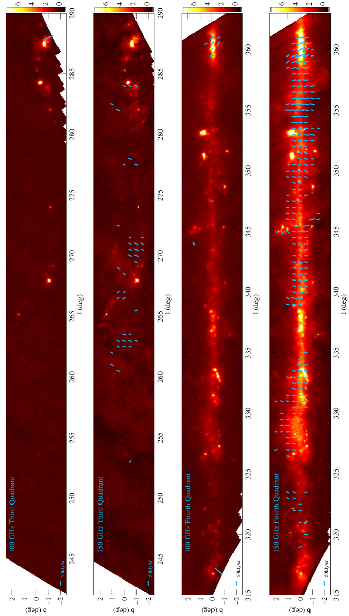
Figure 5.— Total intensity and polarization vector maps for third quadrant 100 GHz (first) and 150 GHz (second), and fourth quadrant 100 GHz (third) and 150 GHz (fourth). The total intensity maps are full-resolution maps smoothed to the beam scale; the color scale is in MJy/sr. The polarization vectors are derived from coarse resolution maps with $0.5^{\circ}$ pixels. Only polarization vectors for which $P/\sigma_{P}>5$ are shown.

5. Properties of Diffuse Emission

The QUaD data can be used to place constraints on interesting properties of the bulk galactic emission, namely the total intensity spectral index, the polarization fraction, and the angle of polarization. Due to the low signal-to-noise of polarization, we use the coarse resolution maps described above for the analysis; for convenience, the maps are interpolated to galactic coordinates as described in Section 4.4. On the coarse pixel grid, the effects of differing beam sizes between the two frequency bands become negligible compared to the effects of pixelization.

Figure 5 shows polarization vectors from the coarse maps overlaid on full resolution total intensity maps for the $|b|<2.5^{\circ}$ region of the survey. Pixels with polarized intensity signal-to-noise $P/\sigma_{P}>5$ have been excluded, with the polarized intensity

$$P^{2}=Q^{2}+U^{2}$$ (2)

and its error given by

$$\sigma_{P}^{2}=\sigma_{Q}^{2}+\sigma_{U}^{2}+2\sigma^{2}_{QU},$$ (3)

where $\sigma_{Q}^{2}$ and $\sigma_{U}^{2}$ are the variances in Q and U, and $\sigma_{QU}$ is the covariance between Q and U map pixels. The 150 GHz  data in particular show a high degree of alignment between the polarization (pseudo) vectors. In the statistical analysis that follows, pixels from the third and fourth quadrant maps are combined. Throughout, we ignore the contribution of primordial CMB anisotropies; the bulk of the analysis is performed within $-1^{\circ}<b<1^{\circ}$, where the galactic emission is expected to be overwhelmingly dominant in both total and polarized intensity. In addition, pixels whose polarized emission is dominated by discrete sources rather than the diffuse background are also excluded. This flagging only includes the galactic center and a polarized cloud at $l\sim 345^{\circ}$, $b\sim 1.75^{\circ}$. To determine bulk emission properties, the analysis which follows makes use of the formalism presented in Weiner et al. (2006), who define a generalised $\chi^{2}$ statistic $L$ which accounts for errors in both coordinates $e_{x}$ and $e_{y}$, and intrinsic scatter $\sigma_{y}$ in a linear model $y=A+Bx$:

$$L=\sum_{i}-\frac{1}{2}\ln 2\pi\left(B^{2}e^{2}_{x,i}+e^{2}_{y,i}+\sigma^{2}_{y}\right)+\frac{\left(y_{i}-\left(A+Bx_{i}\right)\right)^{2}}{B^{2}e^{2}_{x,i}+e^{2}_{y,i}+\sigma^{2}_{y}}.$$ (4)

$L$ is minimized using standard routines that return errors on the fit parameters $A$, $B$ and $\sigma_{y}$; these errors are also verified by using bootstrap realizations of the data. Pixel values are the $x_{i}$ and $y_{i}$, with their errors $e_{x,i}$ and $e_{y,i}$ determined from the variance maps. The intrinsic scatter term accounts for the variation in sky signal above that expected from the instrumental noise alone. For the purposes of quick reference, a summary of the diffuse analysis is presented in Table 1.

Table 1Average Diffuse Emission Properties

Property	100 GHz		150 GHz
	$\bar{x}$	$\sigma_{x}$	$\bar{x}$	$\sigma_{x}$
$\alpha_{I}$	$2.35\pm 0.01\pm 0.02$	$0.158\pm 0.004$	…	…
$P/I$ (%)	$1.38\pm 0.08\pm 0.1$	$0.74\pm 0.03$	$1.70\pm 0.06\pm 0.1$	$1.83\pm 0.06$
$\phi$ (deg)	$4.1\pm 1.3\pm 5$	$33.7\pm 1.0$	$7.0\pm 1.1\pm 2$	$29.7\pm 0.9$

Note. — Summary of average diffuse emission properties from QUaD data. The symbols $\bar{x}$ and $\sigma_{x}$ represent the mean and intrinsic scatter of each quantity in the leftmost column; where quoted, the first error is statistical and the second systematic.

5.1. Total Intensity Spectral Index

The spectral index in total intensity is calculated by minimizing Equation 4 to find the slope $B$ (with the intercept $A$ held fixed) between the $y_{i}=I_{150,i}$ and $x_{i}=I_{100,i}$ pixels. Pixels used in this analysis are restricted to those with $|b|\leq 1^{\circ}$, where the effects of data processing are smallest — see Appendix A.3. The slope is simply related to the spectral index as

$$\alpha_{I}=\frac{\ln B}{\ln(150/100)},$$ (5)

where the spectral index is calculated at the nominal QUaD center frequencies. These are assumed fixed, regardless of the spectral index of the underlying emission mechanisms — a more rigorous analysis would involve integrating each source model over the bandpass and re-calculating the central band frequencies, as the source spectral index can cause $\nu_{0}$ to shift. We determined that for reasonable values of the source spectral index, $\nu_{0}$ varies by only a few percent, changing our results insignificantly compared to absolute calibration errors. Converting to spectral index via Equation 5, the best fit parameters are $\alpha_{I}=2.38\pm 0.01\pm 0.02$, and $\sigma_{\alpha{I}}=0.158\pm 0.004$. The first error on $\alpha_{I}$ is statistical, while the second is systematic as estimated from signal-only simulations (see Appendix B.1).

To test for spectral index variations as a function of galactic latitude, the pixels are subdivided into rows of constant $b$, and the analysis above repeated. Figure 6 shows the results: The spectral index appears to flatten between $+1^{\circ}$ and $-1^{\circ}$, moving from $\alpha_{I}\sim 2.4$ to $\alpha_{I}\sim 1.8$. In principle, the field-differencing, filtering and destriping processes could cause this measurement to be biased due to systematic effects. However, signal-only simulations described in Appendix B.1 show that these processes introduce a systematic shift of $<1\%$ and a scatter of $\sim 7\%$ to the spectral index measurement. Variation of $\alpha_{I}$ with $b$ in the QUaD data is therefore likely a real property of the galaxy.

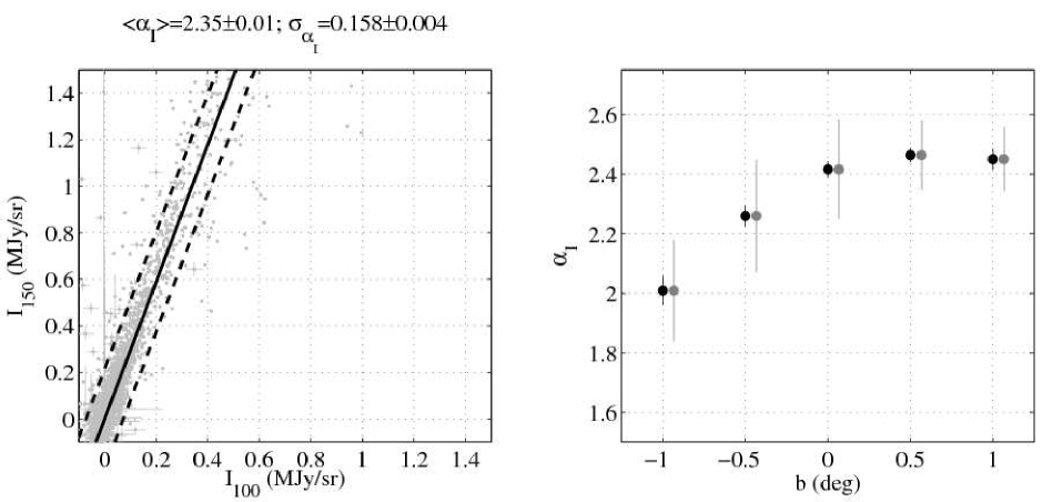
Figure 6.— Left: scatter plot of 150 GHz vs 100 GHz I pixels. The solid black line is the best fit mean slope $B=I_{150}/I_{100}$, with the broken black lines indicating the $\pm 1\sigma_{B}$ regions described by the intrinsic scatter of the data. $B$ and $\sigma_{B}$ are converted to spectral index $\alpha_{I}$ and intrinsic scatter $\sigma_{\alpha_{I}}$, with the best fit values and errors for these parameters shown above the plot. Right: $\alpha_{I}$ as a function of galactic latitude $b$. The black dots show the mean value and its error, while the gray error bars indicate the intrinsic scatter $\sigma_{\alpha_{I}}$.

The QUaD value of the spectral index between 100 and 150 GHz is lower than that expected for dust alone ($\alpha_{d}\simeq 4$), implying one (or more) additional emission component is present. Possible candidates for the extra component are synchrotron, free-free or spectral line emission. Synchrotron has a steeply falling spectral index ($\alpha_{s}\sim-0.7$), but is not expected to dominate near the plane on account of its large scale height. Alternatively, free-free emission has a flatter spectral index ($\alpha_{ff}\sim-0.1$) and is concentrated towards $b=0$ due to the collisional nature of the process. Given the expected spectral indices of these components, it is likely an excess of emission in the 100 GHz band (rather than a 150 GHz deficit) that causes the relatively flat QUaD spectral index. Spectral line emission is a further possibility, with several authors reporting large line contributions to the bolometric flux, though at higher frequencies  (e.g. Groesbeck, 1995; Comito et al., 2005; Wyrowski et al., 2006). The two QUaD bands alone are insufficient to separate these components; a discussion of spectral fitting in conjunction with the WMAP data is deferred to Section 5.3, while Section 5.4 discusses the relative contributions of synchrotron, dust and free-free as predicted from models.

5.2. Polarization

Two quantites are of interest from the polarization data: the polarization fraction, and the angle of polarization. The analysis of polarization fraction proceeds similarly to the spectral index. This time, we search for the gradient and intrinsic scatter in a plot of Q or U  against I via minimization of Equation 4; the intercept is fixed at zero as before. Appendix B.2 demonstrates that field-differencing, filtering and mapmaking processes bias the recovery of $Q/I$ or $U/I$ by $\sim 0.1\%$.

For the polarization fraction analysis, the jackknife maps are also used to test for contamination; the analysis is identical to the signal data. Note that the polarization fraction for jackknife pixels is defined as

$$\left(\frac{Q}{I}\right)_{jack}=\frac{Q_{jack}}{I_{signal}},$$ (6)

and likewise for U, where $I_{signal}$ is the un-jackknifed total intensity map. Ideally there is no sky signal in the jackknife maps, and hence Equation 6 represents the polarization fraction that would have been observed if the sky had a true polarization fraction of zero.

The average 100 GHz polarization fractions are $Q/I=1.38\pm 0.06$% with $\sigma_{Q/I}=0.54\pm 0.02$% for the intrinsic variance, and $U/I=-0.12\pm 0.05$% with $\sigma_{U/I}=0.51\pm 0.02$%. At 150 GHz, $Q/I=1.68\pm 0.04$% with $\sigma_{Q/I}=1.37\pm 0.04$%, and $U/I=0.27\pm 0.04$% with $\sigma_{U/I}=1.22\pm 0.04$%. Combining these results and subtracting the noise bias in $P$ (i.e. $P_{debias}=\sqrt{P^{2}-\sigma^{2}_{P}}$), we find average polarization fractions of $P/I=1.38\pm 0.08\pm 0.1$% at 100 GHz and $P/I=1.70\pm 0.06\pm 0.1$% at 100 and 150 GHz respectively, where the first error is random and the second due to systematic effects as determined from signal-only simulations (Appendix B.2). The corresponding intrinsic scatter is simply computed as the quadrature sum of that from $Q/I$ and $U/I$, and is $0.74\pm 0.03$ and $1.83\pm 0.06$ at 100 and 150 GHz respectively.

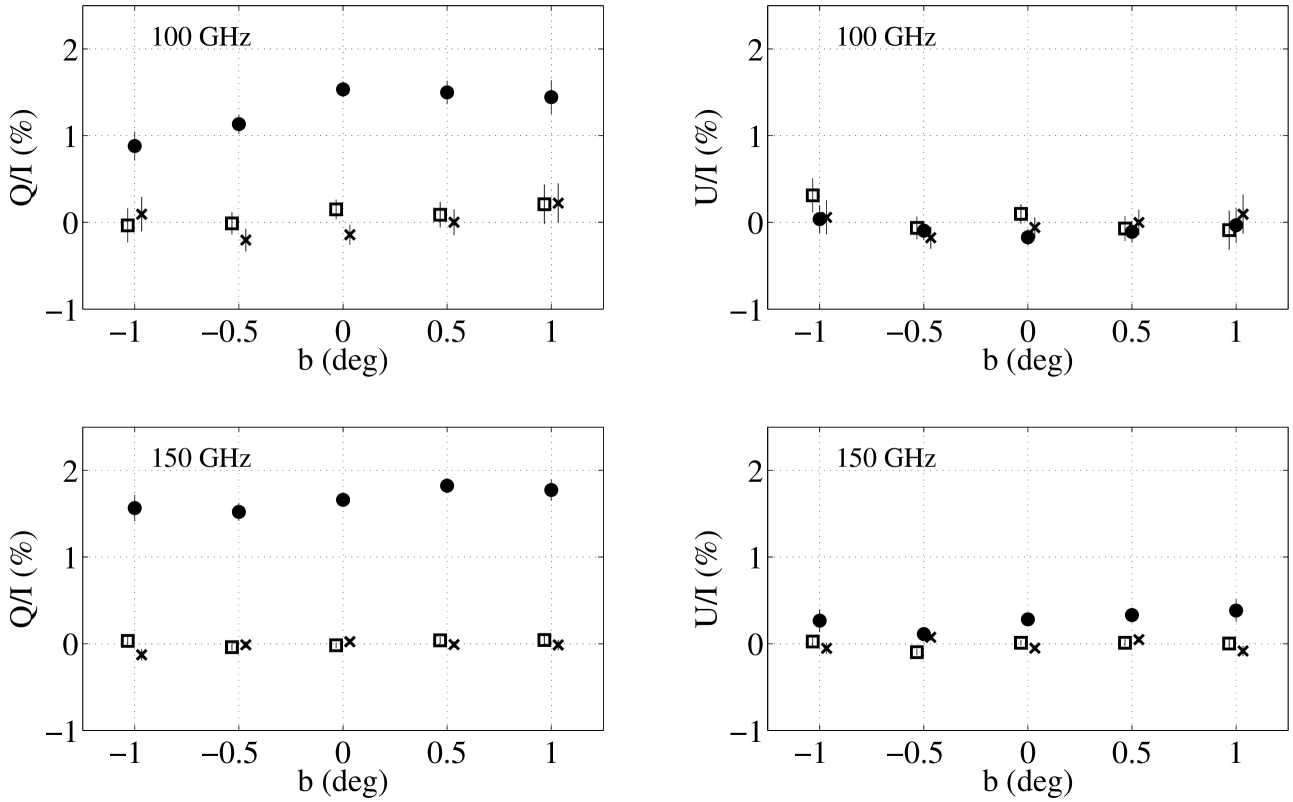
Figure 7.— QUaD measurement of galactic-longitude averaged polarization fraction as a function of galactic latitude. Top row is 100 GHz $Q/I$ (left) and $U/I$ (right); the QUaD signal data are black points, with the scan direction and time jackknife are squares and crosses respectively (the jackknife data are offset in $b$ from the signal data for clarity). Bottom row is for 150 GHz.

Figure 7 displays the average $Q/I$ and $U/I$ polarization fraction of diffuse emission as a function of galactic latitude for the QUaD signal and jackknife data. The signal data shows polarization fractions which are close to constant with $b$. The mean value in each jackknife $b$ bin is expected to be consistent with zero for both $Q/I$ and $U/I$, with the variance due to pixel noise only — Figure 7 shows that this is largely the case, with the jackknife data in each bin consistent with zero at the $2\sigma$ level or better.

The $P/I$ values of polarization fraction are somewhat lower than the Archaeops result (Benoît et al., 2004), who found a 4-5% polarization fraction for $|b|<2^{\circ}$ over the galactic longitude range 297 to 85^∘ at 350 GHz. Conversely, using WMAP 3 year data, Kogut et al. (2007) found a 94 GHz polarization fraction closer to $\sim 1\%$ averaged over a region including the QUaD survey between galactic latitudes $-10<b<10^{\circ}$, rising to 3.6% outside the P06 mask used in their analysis. A direct comparison of QUaD to the WMAP data is presented in Section 5.3.

If the large-scale magnetic field is largely aligned in the plane of the galaxy, in the galactic coordinate system this translates to polarized emission predominantly in $+Q$. Figure 7 demonstrates that this is observed by QUaD, though the $U/I$ data at 150 GHz shows detected signal. This observation may be alternatively quantified by directly computing the polarization angle $\phi=0.5\mathrm{tan}^{-1}\left(U/Q\right)$ and its error $\mathrm{d}\phi=0.5(1+U^{2}/Q^{2})^{-1}\mathrm{d}(U/Q)$, where

$$\mathrm{d}\left(U/Q\right)=\left(U/Q\right)\sqrt{\left(\frac{\mathrm{d}Q}{Q}\right)^{2}+\left(\frac{\mathrm{d}U}{U}\right)^{2}}.$$ (7)

The effective $\chi^{2}$ function in Equation 4 is then minimized — this time, since we wish to know the mean and intrinsic variance of the $\phi$ distribution, the gradient term $B$ is fixed at zero. The analysis is performed on the same pixels as polarization fraction, with the mean and intrinsic variance calculated for all pixels and in rows of constant $b$. Figure 8 shows the results. The mean polarization angles are $\phi_{100}=4.1\pm 1.3^{\circ}\pm 5^{\circ}$ and $\phi_{150}=7.0\pm 1.1^{\circ}\pm 2^{\circ}$, with intrinsic variance $\sigma_{\phi,100}=33.7\pm 1.0^{\circ}$ and $\sigma_{\phi,150}=29.7\pm 0.9^{\circ}$. For $\phi$, the second error is the estimated systematic uncertainty in the polarization angle using signal-only simulations (see Appendix B.2). In bins of constant galactic latitude, $\phi$ and its intrinsic variance do not vary significantly. A weighted probability distribution of $\phi$ is also shown at each frequency for the signal data, and all jackknife data combined. At both frequencies, a distinct peak is observed in the distribution close to the mean values calculated above, while the jackknifes are consistent with random numbers distributed uniformly between $-90^{\circ}<\phi<90^{\circ}$, as expected in the presence of no signal.

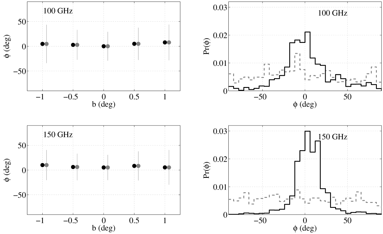
Figure 8.— QUaD polarization angle; top and bottom are 100 and 150 GHz respectively. Left: $\phi$ vs $b$ in 0.5^∘ bins of galactic latitude. Black points show the mean $\phi$ in each bin, while black and gray error bars indicate the statistical error on the mean and the intrinsic scatter respectively. Right: weighted probability distribution $Pr(\phi)$ of the pixel values as a function of $\phi$. The black solid line corresponds to the data, while the broken gray line shows Pr($\phi$) for the combined jackknife maps. The QUaD data clearly show a peak in Pr($\phi$) compared to the jackknife data, indicating the presence of coherent polarized galactic signal.

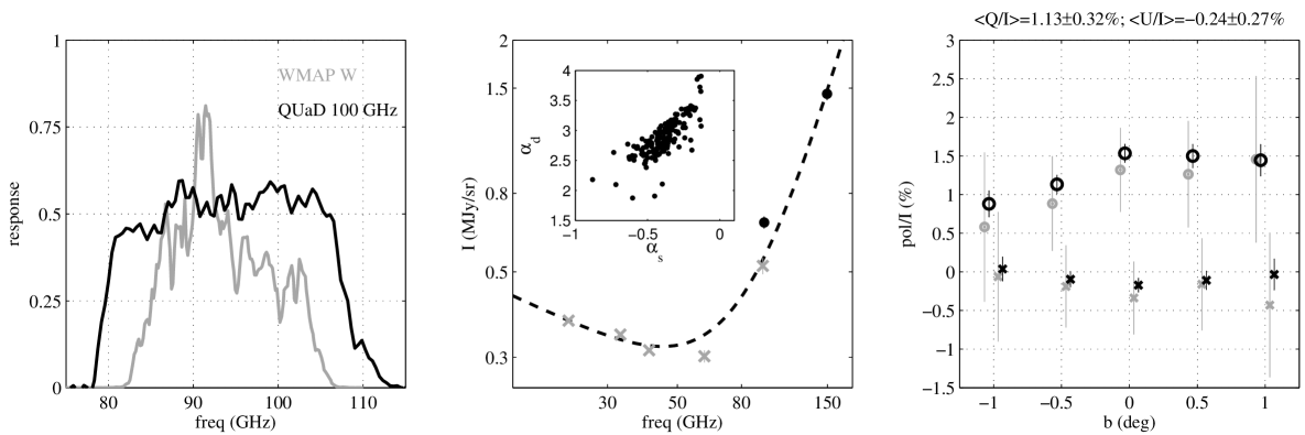
Figure 9.— Left: QUaD 100 GHz and WMAP W bandpass spectral response in black and gray respectively. The QUaD band is substantially wider, with $\Delta\nu=27$ GHz compared to $\Delta\nu=20$ GHz for WMAP W band. Center: Example data points and spectral fit for a representative pixel in the WMAP and QUaD maps. WMAP data are gray crosses, QUaD data are black dots, and the broken black line indicates the best-fit two-component spectrum. The inset shows the distribution of spectral indices taken over map pixels used in the analysis. Right: Average polarization fraction as a function of galactic latitude. Gray is WMAP, black is QUaD 100 GHz for comparison; circles are Q, crosses are U. The points have been offset in $b$ for clarity.

The QUaD data indicate that while the galactic magnetic field is preferentially aligned parallel to the plane, there is significant additional scatter present. However, signal-only simulations (Appendix B.2) show that a substantial contribution to the scatter in the angle may be present due to filtering and processing and effects. At 100 GHz this systematic scatter is comparable to the observed scatter, indicating we cannot reliably constrain $\sigma_{\phi}$ at this frequency.

5.3. Comparison to WMAP

The closest comparison to the QUaD 100 GHz data is from WMAP W band, centred on 94 GHz. For the following analysis, the 5-year WMAP data (Hinshaw et al., 2009) are used to generate simulated timestream in the regions observed by QUaD. The timestream is processed in the same manner as the signal-only simulations described in Appendix A, in which the field-differencing and filtering operations are performed exactly as for the QUaD data.

The combination of QUaD and WMAP total intensity data allows constraints on the spectral index of emissive components in the galaxy. Using the QUaD and WMAP beam and pixelization functions, the WMAP Ka, Q, V and W band maps, and the QUaD survey, are convolved to the WMAP K-band resolution of $0.93^{\circ}$, and binned into the $0.5^{\circ}$ pixels used in the coarse resolution QUaD maps. Pixel noise in the WMAP maps are determined from regions well away from the galactic plane, but are much smaller than the absolute calibration uncertainties of the smoothed maps. Using the same pixel from each map, the data from each of the seven bands are fit to a two-component continuum model, the sum of two power laws in frequency $\nu$:

$$I(\nu)=A_{s}\nu^{\alpha_{s}}+A_{d}\nu^{\alpha_{d}}.$$ (8)

In this expression, $\alpha_{s}$, and $\alpha_{d}$ are the synchrotron and dust spectral indices respectively. Note that the first component is only loosely termed as due to synchrotron; as discussed previously, free-free is likely the second most dominant emission mechanism after dust at 60–100 GHz. To fit the data, the model is convolved across each bandpass to yield the average intensity in that band:

$$\tilde{I}_{\nu}=\frac{\int I(\nu)T(\nu)d\nu}{\int T(\nu)d\nu},$$ (9)

where $T(\nu)$ is the bandpass response as a function of frequency, as shown for WMAP W band and QUaD 100 GHz in the left panel of Figure 9. The $\chi^{2}$ against the data is calculated and minimized to find the best-fit parameters for the model in Equation 8, with Equation 9 evaluated for every set of trial parameters used in the minimization.

The QUaD data is $\sim 25\%$ brighter than WMAP at similar frequencies, indicating a discrepency between the two experiments which is further discussed in Section 5.4. The center panel of Figure 9 shows the fit spectrum for a single representative pixel in the data, and a scatter plot of $\alpha_{s}$ against $\alpha_{d}$ for the spectral fit to each map pixel. Taken over all pixels, the average spectral indices are $\alpha_{s}=-0.32\pm 0.03$ and $\alpha_{d}=2.84\pm 0.03$. The former is flatter than might be expected for pure synchrotron ($\alpha\sim-0.7$), indicating the presence of free-free and/or dust, while the latter is lower than that predicted by the FDS dust model 8 ($\alpha_{d,FDS}=3.5$; see Appendix B.1). It is clear that the simple two-component model used is inadequate to describe the data; this statement remains true if the QUaD 100 GHz data is excluded. In fact, Gold et al. (2009) find that inside the plane (interior to the WMAP 5 year KQ95 mask), a ten-parameter model is insufficient to fully describe their data, and therefore it may be optimistic to expect simple models to account for all emission along lines of sight close to the plane.

The right panel of Figure 9 compares the polarization fraction, averaged along galactic longitude, between the unsmoothed WMAP W band maps, and QUaD 100 GHz— both maps are binned at $0.5^{\circ}$ resolution. The plot demonstrates that QUaD is consistent with the WMAP observations to within $1\sigma$, in both Q and U, with WMAP mean values of $Q/I=1.13\pm 0.32\%$ and $U/I=-0.24\pm 0.27\%$ ($P/I=1.1\pm 0.4\%)$, compared to $1.38\pm 0.06\%$ and $-0.12\pm 0.05\%$ for QUaD ($P/I=1.38\pm 0.08\%)$; agreement between the two datasets is also found as a function of galactic latitude.

5.4. Comparison to Emission Models

Synchrotron and dust models are provided by Finkbeiner (2001) and Finkbeiner et al. (1999) (we use dust model 8 in the latter case); these can be extrapolated into the QUaD bands and compared to the observations. At frequencies $\sim$100 GHz, free-free emission is also expected to contribute. The H$\alpha$ sky template provided by Finkbeiner (2003) is used to generate a free-free emission map at the QUaD frequencies; we follow Schäfer et al. (2006), who convert the H$\alpha$ template from Rayleigh units into $\mu$K using the formula provided by Valls-Gabaud (1998):

$$\frac{T_{free-free}(\mu\mathrm{K})}{A_{H\alpha}(R)}\simeq 14.0\left(\frac{T_{p}}{10^{4}K}\right)^{0.317}10^{\frac{290}{T_{p}}}g_{ff}\left(\frac{\nu}{\mathrm{10GHz}}\right)^{-2},$$ (10)

where $A_{H\alpha}$ are the template pixel values in Rayleighs, $T_{p}$ is the plasma temperature (assumed to be $10^{4}$K), $\nu$ is the central observing frequency of the QUaD bands, and $g_{ff}$ is the free-free Gaunt factor as calculated in Finkbeiner (2003). The temperature maps are converted to brightness units as in Equation 1.

Signal-only simulations of synchrotron, dust and free-free are used to generate field-differenced and filtered maps of these components, which are then summed to produce a model sky at QUaD frequencies. The limiting factor in resolution is the synchrotron model, which is derived from 405 MHz maps of Haslam et al. (1981, 1982) with a beam FWHM of $\sim 1^{\circ}$. QUaD and model maps are binned into $0.5^{\circ}$ pixels and smoothed to $1^{\circ}$ resolution to match the synchrotron model.

In Figure 10 we plot the pixel values between QUaD and the model predictions against each other (left panels), and the mean ratio of pixel values between QUaD and the models $R=I_{QUaD}/I_{model}$ in bins of $b$ (right panels). $R$ is the gradient in a plot of $I_{QUaD}$ against $I_{model}$; this is calculated for all pixels and as a function of $b$ by minimizing Equation 4, holding the intercept fixed as in Section 5.1 with intrinsic scatter fitted simultaneously. The models are split into three compositions: dust alone, dust+synchrotron, and dust+synchrotron+free-free, with comparisons to QUaD data made for each.

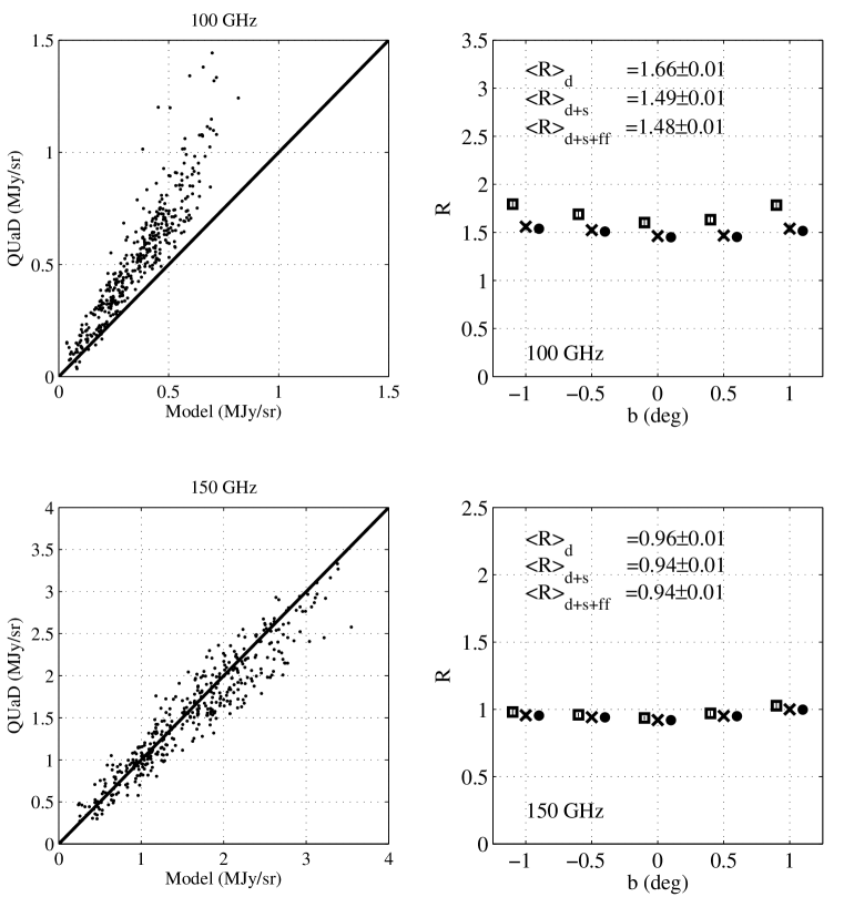
Figure 10.— Left panels: QUaD pixel values plotted against signal-only simulations of the model including dust, synchrotron, and free-free as described in the text; top is 100 GHz, bottom is 150 GHz. Right panels: Ratio of QUaD map pixel values to model predictions at 100 (top) and 150 GHz (bottom), as a function of galactic latitude. Square symbols compare QUaD to the FDS dust model, crosses are dust+synchrotron, and dots correspond to dust+synchrotron+free-free.

At 100 GHz, QUaD is brighter than the FDS dust-only prediction by a factor $1.66\pm 0.01$, decreasing to $1.49\pm 0.01$ and $1.48\pm 0.01$ as synchrotron and free-free models are added; the intrinsic scatter is $\sim 0.1$ for all models. This extra signal at 100 GHz is hereafter referred to as the ‘QUaD excess’ — we note that Gold et al. (2009) also find an excess of observed W band emission over that predicted by the Finkbeiner et al. (1999) models over most of the sky. At 150 GHz the model predictions are in better agreement with QUaD; $R$ ranges from $0.962\pm 0.007$ (dust only) to $0.942\pm 0.006$ (all model components), with the intrinsic scatter $\sim 22\%$. The ratio $R$ only changes by $1$–$2\%$ comparing QUaD to the model with dust only or all components at this frequency; this is to be expected since dust dominates the emission at 150 GHz. At both frequencies, $R$ does not vary strongly with galactic latitude, though care should be taken when interpreting these results since the maps are smoothed to $1^{\circ}$ resolution, and thus the data points are highly correlated between $-1^{\circ}<b<1^{\circ}$.

It should be noted a factor $\sim 2$ uncertainty exists in the conversion factor from Rayleigh units to antenna temperatures which we apply to the Finkbeiner (2003) free-free maps, which could contribute to the QUaD 100 GHz excess. However, Figure 10 shows that the addition of a free-free template to a dust+synchrotron model changes the ratio of QUaD to model pixel values by less than 1%; thus even a factor $2$ underestimation of the free-free model calibration is insufficient to account for the excess emission.

Another possible explanation of the QUaD excess is molecular line emission: large fractional contributions from line emission have been measured at higher frequencies towards star-forming regions (e.g. Groesbeck, 1995; Nummelin et al., 1998); these can range from $10-65\%$ of the bolometric intensity. On the other hand, the COBE FIRAS instrument has detected much lower line emission contributions ($<$1%) over large patches of sky (e.g., Wright et al., 1991; Bennett et al., 1994; Fixsen et al., 1999).

If the line emission interpretation is correct, one might expect the QUaD 100 GHz data to be brighter than WMAP W band on account of the wider bandwidth admitting more lines (see Figure 9), and the WMAP data to be brighter than the models which do not include line emission at all. This trend is indeed observed: QUaD 100 GHz data is a factor $1.48$ brighter than the model with dust, synchrotron and free-free included, and QUaD 100 GHz is also $\sim 25\%$ brighter than WMAP W band. WMAP is therefore some $23\%$ brighter than the combined models for continuum emission, providing independent evidence that these models are insufficient to describe the data close to the plane of the galaxy.

5.5. Tests of the Spectral Line Hypothesis

Given the variation seen in the literature on spectral line contributions at higher frequencies, the hypothesis that line emission causes the QUaD excess is subjected to the following additional tests.

5.5.1 Spectral Comparison Using FIRAS

The FIRAS instrument aboard the COBE satellite provides absolute spectral measurements covering the QUaD 100 GHz band, at a resolution of $\sim 7^{\circ}$. A direct comparison between QUaD and FIRAS is not possible since the FIRAS beam width is half the maximum width (in R.A.) of the QUaD survey, and hence the QUaD maps cannot be smoothed to the same spatial resolution. Neither can spectral discrimination be used to compare the FIRAS data as filtered through the QUaD and WMAP bandpasses, since even at maximum spectral resolution of 3.4 GHz, the frequency sampling is too sparse to resolve the difference between QUaD and WMAP where there is no spectral overlap. However, the FIRAS data can be used to obtain an upper limit on the emission expected in the QUaD 100 GHz band, providing a useful consistency check of the QUaD absolute calibration. We restrict ourselves to pixels less that $5^{\circ}$ from the galactic plane, and subtract the best-fit CMB monopole blackbody spectrum from each FIRAS frequency channel. Other filtering effects such as polynomial subtraction are not included because the large FIRAS beam smooths the galactic signal to greater galactic latitudes than covered in the QUaD survey. Polynomial subtraction of the signal lying at the QUaD scan ends would then reduce the amplitude below the level of signal loss due to filtering in the QUaD survey itself.

The signal-to-noise at $\sim$100 GHz is low in the FIRAS data, so an upper limit is obtained by finding the 95th percentile of the pixel distribution for each frequency channel. This ‘spectrum’ of 95th percentiles is then integrated over the normalized QUaD 100 GHz bandpass, resulting in an upper limit of 5.3 MJy/sr at 95% confidence. This limit is consistent with the QUaD data; Figure 5 shows that at 100 GHz the peak brightness is $\sim 7\mathrm{MJy/sr}$ near the galactic center, which would be reduced by the ratio of beam areas (a factor $\sim(7\times 60/5)^{2}=7056$) once beam smoothing is taken into account. Therefore the FIRAS data cannot isolate the QUaD excess as being due to spectral lines or an absolute calibration mismatch.

5.5.2 Spectral Comparison Using CO 1-0 Transition Maps

The most prominent line near the lower QUaD band is the 1–0 CO transition at $\sim 115$ GHz. This has been mapped over the inner galactic plane by Dame et al. (2001) and references therein; the survey has spatial resolution $6^{\prime}$, very close to QUaD at 100 GHz. As seen in Figure 9, the QUaD band response at 115 GHz is small (a factor of $\sim 1000$ smaller than the peak in fact). The CO maps are restricted to the QUaD survey boundaries, and the antenna temperature units converted to MJy/sr, first by converting antenna temperatures to thermal temperature units for each frequency channel, and then by averaging the CO data in frequency over the spectral bandwidth, and finally averaging over the QUaD bandpass. We find a peak CO contribution of $10^{-2}~{}\mathrm{MJy/sr}$, or approximately 2% of the typical brightness of a WMAP pixel in the QUaD survey region, and is therefore insufficient to account for the $\sim 25\%$ excess seen by QUaD over WMAP.

5.5.3 Spectral Line Check Using Polarization

Spectral lines are not expected to emit polarized radiation, so any contribution can be tested by comparing the unpolarized and polarized data.

The left panel of Figure 11 shows a plot of QUaD 150 vs. 100 GHz data in I and Q. The slope in I is clear, and is apparently traced by Q; this indicates that line emission does not contribute significantly to the lower QUaD band, as otherwise a steeper slope would be expected in polarization. However, the signal-to-noise at 100 GHz is low: Also plotted in Figure 11 are the pixel values from the scan-direction jackknife, which demonstrate that instrumental noise contributes significantly to the 100 GHz data, and therefore statistical uncertainties could bias the polarized spectral index measurement towards lower values.

Greater signal-to-noise can be acheived by using the galactic longitude-averaged data. Neither dust nor synchrotron are expected to vary polarization fraction with frequency, yet as seen in Table 1 and Figure 11, the observed polarization fractions differ between QUaD bands. Taking the average values of $P/I$ at each frequency, the unpolarized spectral index, and combining the measurement uncertainties and intrinsic scatter into a single error term, we find $\alpha_{P}=2.81^{+0.26}_{-0.25}$. This is discrepent with the total intensity spectral index at the $\sim 2\sigma$ level, and is thus an inconclusive test on the existence or not of additional emission components.

As a final test, the QUaD 100 GHz maps are compared to WMAP W band in Stokes Q on a pixel-by-pixel basis. The right panel of Figure 11 shows such a plot of this test; both data sets are noisy and a statistically significant measurements of the gradient is not possible. Instead, we simply take the mean of each set of pixels and calculate the ratio, finding $\langle Q\rangle_{QUaD}/\langle Q\rangle_{WMAP}=1.4\pm 0.5$. Such large errors render the data insufficient to measure an excess of QUaD polarization over WMAP, and thus cannot verify or falsify a contribution due to line emission or an absolute calibration mismatch.

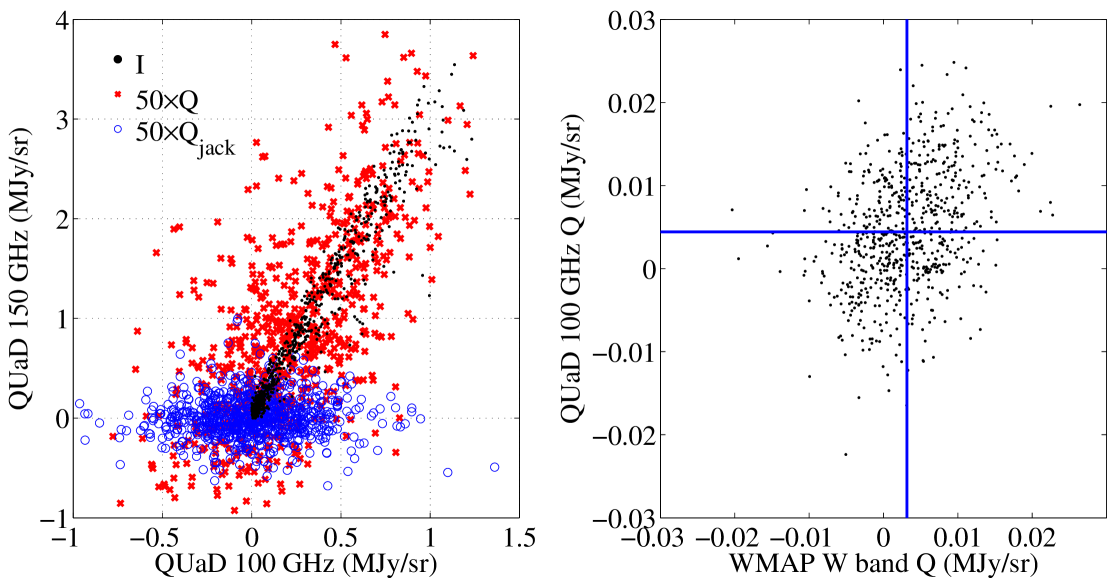
Figure 11.— Left: Scatter plot of QUaD 150 vs. 100 GHz data. Black points are for unpolarized intensity I, red are for Q, and blue are for the scan-direction Q jackknife to indicate the level of noise present in the QUaD 100 GHz Q data. The polarization data have been multiplied by 50 for visual display purposes only. Right: Scatter plot for QUaD 100 GHz data against WMAP W band for Stokes Q. The solid lines indicate the mean value of each data set.

6. Conclusions

We present the QUaD survey of the Milky Way in Stokes $I$, Q and U, with a resolution of 5 (3.5) arcmin at $100$ and 150 GHz respectively. The survey covers two regions, $110^{\circ}<\mathrm{RA}<190^{\circ}$ and $210^{\circ}<\mathrm{RA}<290^{\circ}$, both in the dec range $-60.5^{\circ}<\mathrm{dec}<-26.5^{\circ}$, corresponding to approximately $245-295^{\circ}$ and $315-5^{\circ}$ in galactic longitude, and $-4<b<4^{\circ}$ in galactic latitude — a total of $\sim 800$ square degrees.

Degrading the map resolution to $0.5^{\circ}$ pixels, the average spectral index of diffuse emission is $\alpha_{I}=2.35\pm 0.01\mathrm{(stat)}\pm 0.02\mathrm{(sys)}$, assuming nominal band centers of 94.5 and 149.6 GHz. This value of spectral index is flatter than that expected from dust alone — Gold et al. (2009) demonstrate that the WMAP 5 year data only weakly constrains the dust spectral index, but use a prior range $3.5<\alpha_{d}<5$, indicative of the expectation for this component. The low QUaD-only value is interpreted as evidence for additional emission components in the lower frequency QUaD band.

A direct comparison to WMAP 5 year W band data shows the QUaD 100 GHz maps are on average $\sim 25\%$ brighter. Fitting a two-component continuum model to all pixels in the five WMAP and two QUaD bands results in constraints of $\alpha_{s}=-0.32\pm 0.03$ and $\alpha_{d}=2.84\pm 0.03$. The first is attributed to a composite of synchrotron, free-free and dust expected at $\sim 100$ GHz close to the galactic plane, with the second interpreted as mostly dust. However, the fit is poor for such a simple model and more emission components would be required to fully explain the data.

Similarly to the spectral index determined from QUaD alone, $\alpha_{d}$ is lower than the expectation from available models. A composite model of dust, synchrotron and free-free emission underestimates the brightness at 100 GHz, where QUaD observes on average a factor $1.48\pm 0.01$ more signal. One interpretation of this effect is molecular line emission. This possibility is discussed further in Section 5.5, where a variety of cross-checks indicate that the 115 GHz CO 1-0 line is unlikely to be the main cause of the 100 GHz excess, but that the QUaD data are consistent with absolute spectral measurements from the COBE FIRAS instrument. At 150 GHz  the agreement is better, with an average pixel ratio of $0.942\pm 0.006$ between QUaD and the models.

The QUaD data allow measurement of the polarization fraction in both bands — the results quoted here are taken from galactic coordinates maps using the IAU convention for Stokes parameters $Q$ and $U$. Analysis in the Source Paper shows that few compact objects have measurable polarization and thus we assume the dominant source of the polarized emission studied here is diffuse. On average, $Q/I=1.38\pm 0.06$% and $1.68\pm 0.04$% at 100 and 150 GHz, with the equivalent averages for $U/I$ being $-0.12\pm 0.05$% and $0.27\pm 0.04$%. The intrinsic scatter on these quantities were found to be typically $\sim 0.5$ ($\sim 1.3$)% at 100 and 150 GHz respectively, reflecting fluctuations in polarization fractions at different positions in the galactic plane. Signal-only simulations indicate that the systematic error on polarization fraction is of order $0.1\%$ at both frequencies. Measurements of $Q/I$ and $U/I$ are also possible as a function of galactic latitude $b$ within $|b|\leq 1^{\circ}$, and show evidence of small deviations from the average polarization fractions quoted above, but within the range allowed by the intrinsic scatter. Combining $Q/I$ and $U/I$, we find total polarization fractions $P/I=1.38\pm 0.08\pm 0.1$% at 100 GHz and $1.70\pm 0.06\pm 0.1$% at 150 GHz, where the first error is random and the second systematic. The intrinsic scatter at these frequencies is $0.74\pm 0.03$ and $1.83\pm 0.06$.

Comparing the QUaD polarization fraction to that from WMAP 5 year data, agreement is found between the two datasets at QUaD 100 GHz and WMAP W band, the latter giving an average polarization fraction $1.1\pm 0.4$%. The polarization fraction measurements reported here provide encouragement that large areas of sky may be useful for probing inflationary cosmology with CMB polarization B-modes at frequencies above 100 GHz.

The mean angle of polarization close to the plane measured by QUaD is is $<\phi>=4.1\pm 1.3\pm 5^{\circ}$ at 100 GHz, with $<\phi>=7.0\pm 1.1\pm 2^{\circ}$ at 150 GHz, where the first error is random and the second systematic. Although the data indicate QUaD has detected intrinsic scatter in the distribution of $\phi$, the amount of scatter is consistent with that introduced by filtering and map processing effects. The observations therefore provide evidence of the large-scale alignment of the galactic magnetic field.

Extensive tests could not definitively isolate the cause of the QUaD excess signal observed over WMAP W band and continuum emission models at 100 GHz. The QUaD data is consistent with an unpolarized intensity upper limit derived from FIRAS data, ruling out a large QUaD absolute calibration error. A second test of the absolute calibration is calculated from the ratio of average Stokes Q in QUaD and WMAP pixels; we find $\langle Q\rangle_{QUaD}/\langle Q\rangle_{WMAP}=1.4\pm 0.5$, an excess over I on average, but statistically consistent with the mean total intensity excess of $\sim 1.25$. Low signal-to-noise in polarization at 100 GHz prevented a direct determination of the polarized spectral index; a larger value than total intensity would be evidence for line emission in the 100 GHz band. Using a combination of the average polarization fraction and the unpolarized spectral index, we determined $\alpha_{P}=2.81^{+0.26}_{-0.25}$, within $2\sigma$ of $\alpha_{I}$ and thus inconclusive regarding molecular line emission. Maps of the CO 1–0 transition (Dame et al., 2001) multiplied through the QUaD bandpass placed an upper limit on the contribution of this molecular line of $10^{-2}~{}\mathrm{MJy/sr}$, which at $\sim 2\%$ of the typical brightness of a WMAP W band pixel is insufficient to account for the QUaD excess. We conclude that higher signal-to-noise measurements of the polarized galactic emission at 100 GHz are required to resolve the QUaD excess, and should be provided in the near future by the Planck satellite (Villa et al., 2002).

This paper focussed on the properties of diffuse emission (typically $0.5^{\circ}$ scales and larger); however, the QUaD galactic plane survey contains information on scales down to 5 and 3.5 arcminutes at 100 and 150 GHz . The small-scale properties of emission via discrete sources are explored in the Source Paper, where a variety of objects have been detected, such as ultra-compact HII regions and supernova remnants.

Appendix A Further Details on Destriping Algorithm

A.1. Map Destriping

When constructing the initial maps $m_{0}$ and $m_{1}$, the choice of polynomial filtering order is a trade-off between increased atmospheric noise reduction (higher order) and reduced filtering of the galactic signal of interest (lower order). A simple DC-level+slope filter function is used in the QUaD survey because we are interested in the emission properties on both small and large angular scales, both of which are suppressed or corrupted by a higher order filter function. However, this choice results in a larger atmospheric noise contribution than would be present had a higher order polynomial been used — the $m_{0}$ map in Figure 3 exhibits large row-to-row striping as a result, which we suppress as follows. After filtering, $1/f$ noise is largely uncorrelated between rows of pixels, while galactic structure is strongly correlated on these angular scales due to its intrinsic structure and beam smoothing. Smoothing the $m_{1}$ maps with a circularly symmetric gaussian kernel of width $4\times\sigma_{beam}$ at each frequency reduces striping between pixels; the smoothed map is treated as a template map of the sky, $m_{t}$. From $m_{t}$, ‘signal only’ timestream $d_{t}$ is interpolated and subtracted from the original data $d$:

$$d_{n}=d-d_{t}.$$ (A1)

The ‘signal-subtracted’ timestream $d_{n}$ is now dominated by atmospheric noise with little galactic signal present, and is fit with a higher order polynomial to measure the atmospheric modes (a 6th-order polynomial is used in the QUaD survey).

Using the resulting polynomial coefficients $p_{n}$, a polynomial $d_{p_{n}}$ which represents atmospheric modes is subtracted from the original unfiltered timestream

$$d_{s}=d-d_{p_{n}},$$ (A2)

and the filtered data is coadded into the map. Since $d_{p_{n}}$ largely measures atmospheric $1/f$ modes, the noise in maps made from $d_{s}$ (denoted $m_{2}$ in the map ordering of our algorithm) is considerably whiter than the $m_{0}$ maps. The improvement may be seen in simulated timestream in Figure 12, and in the resulting maps in Figure 13; the procedure is repeated independently for I, Q and U maps at both frequencies.

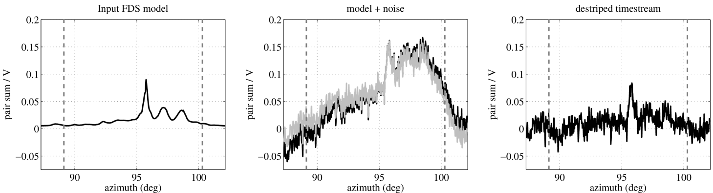
Figure 12.— Destriping process for one half-scan of data for the central 150 GHz  pixel. The dashed graylines show the regions of the scan ends used for DC-level plus slope filtering. Left: Simulated input FDS model 8 signal. Center: Input model plus simulated noise before (black) and after (gray) initial filtering. Right: Destriped timestream — the recovered timestream is an improved estimate of the true sky signal compared to the initial filtering.

Some subtleties are present in this method; since $m_{t}$ is a smoothed version of the sky as observed by QUaD, subtracting it from the timestream introduces residuals near the locations of bright point sources (effectively, subtracting two gaussian functions of equal cross-sectional area but differing widths). These residuals can be large, particularly near the galactic center, influencing the $p_{n}$, causing spurious filtering residuals in the $m_{2}$ maps. This effect is reduced by locating bright sources in $m_{1}$ as described in the Source Paper and then masking them as described below. Since $1/f$ noise in the $m_{1}$ total intensity maps can be spuriously detected as false sources, a high signal-to-noise threshold of $S/N>10$ is used in the I map. For Q and U the noise is considerably whiter, so a threshold of $S/N>3$ is used.

With the locations of bright sources known, two methods are used to reduce their impact on higher-order filtering. First, the source pixels are replaced with a local median and the smoothed template map $m_{t}$ is computed — this reduces the amount of source power smeared out by the smoothing, lowering the corresponding residuals in $d_{n}$. Second, the source locations are masked with a conservative radius of $6\sigma_{beam}$ when performing the 6th-order polynomial fit.

After these steps, the data is filtered as in Equation A2 and coadded into the map, with post-filter inverse scan variances used as weights. Note that the variances for the destriped data are computed over the entire scan after template subtraction and filtering, and with point sources masked, i.e $\sigma^{2}=var(d_{n}-d_{p_{n}})$.

The mapping algorithm implemented in this paper can be summarized as follows:

• Construct $m_{0}$ map from timestream filtered with DC-level+slope determined from scan ends.

• Locate sources using the method described in the Source Paper, mask sources and and repeat Step 1 above to give $m_{1}$.

• Smooth $m_{1}$ with gaussian kernel of $\sigma_{t}=4\times\sigma_{beam}$, with bright source pixels replaced by local median - this is the template map $m_{t}$.

• Interpolate ‘signal-only’ timestream $d_{t}$ from $m_{t}$, and subtract from the original data $d$ to give an approximate ‘noise-only’ timestream $d_{n}$.

• Fit $d_{n}$ with high order polynomial, masking sources located in Step 2. This step measures the ‘noise-only’ polynomial coefficients $p_{n}$.

• Filter the original timestream $d$ using a polynomial with coefficients $p_{n}$, and coadd the filtered half-scans into the map using post-filter inverse half-scan variances as weights; this produces the final $m_{2}$ maps.

Though the destriping algorithm is implemented entirely in timestream/image space, it has a direct interpretation as a linear filter in Fourier space as discussed in Section A.4.

A.2. Test of Mapping Algorithm

To test the algorithm described above, signal-only simulations of the FDS dust model 8 evaluated at the QUaD center frequencies are generated as mock sky signal. We wish to add realistic noise to the simulations, but since the galactic signal can dominate the timestream, we cannot directly take the power spectrum of the data and use it to regenerate noise as in P09 — doing so results in noise strongly correlated with regions of bright galactic emission. To mitigate this effect, the sky signal (as estimated from the destriped maps) is first removed from the data, and the resulting sky-subtracted timestream processed in the same way as P09: continuous segments of data are Fourier transformed, binned, and the covariance matrix of the fourier modes taken between all channels in each bin separately. Noise timestream is then regenerated by mixing uncorrelated random numbers with the Cholesky decomposition of this covariance matrix. Taking the inverse Fourier transform yields simulated noise timestream with the observed degree of covariance as the signal-subtracted data. P09 demonstrates that this process yields simulated noise which is indistinguishable from the real. The simulated noise is added to the signal-only timestream, coadded into $0.02^{\circ}$ maps, and destriped according to Section A.1. Figure 13 shows the signal-only input map $m_{s}$, the DC+slope filtered map $m_{0}$, the destriped map $m_{2}$, and the residual map $m_{2}-m_{s}$. Qualitatively, it is clear that the algorithm is effective at suppressing $1/f$ noise, and introduces small residuals compared to the galactic signal of interest.

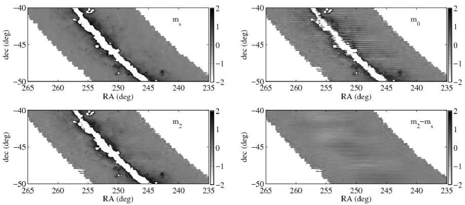
Figure 13.— Maps illustrating the major stages of the mapmaking process. All colorscales are in MJy/sr, with saturated pixels within the survey region shown in white. Top left: Signal-only FDS model 8 prediction at 150 GHz. Top right: signal plus noise simulation of the same model after DC-level + slope filtering, i.e. $m_{0}$ stage map. Bottom left: Recovered $m_{2}$ map after destriping. Bottom right: Difference between input and destriped maps. The color stretch has been reduced by a factor 5 to enhance the residuals; the noise consists mainly of white noise, and large-scale modes which are removed before the destriping in Step 4 of Section A.1.

A.3. Effects of Map/Timestream Processing

The mapmaking algorithm described above results in a loss of signal due to the main stages of processing: field-differencing and destriping. To test the effects of each, the same signal-only simulations of FDS model 8 as in Section A.2 are used, comparing pixel values at each (cumulative) stage of processing of the input maps.

The left panels of Figure 14 show the median fractional change in pixel values of $m_{0}$ maps, before and after field-differencing. At the mean $3\sigma$ noise level in the QUaD maps, field-differencing reduces the signal by $1-7\%$ at 100 GHz, and $5-25\%$ at 150 GHz, depending on dec. The declination dependence arises from the fact that our $15^{\circ}$ azimuth scans correspond to a smaller RA range at lower dec, scaling as $\mathrm{cos}(\mathrm{dec})$. Therefore the low dec trail field scans lie closer to the galactic plane, and so subtract out more sky signal when the lead and trail fields are differenced. The fractional loss in signal is smaller for brighter pixels close to the galactic plane, with less than $5\%$ reduction above 0.35 (1.3) MJy/sr at 100 (150) GHz over all dec.

A similar analysis is shown for the effect of destriping in the right hand panels of Figure 14. Since the destriping method only reduces uncorrelated noise between rows of pixels, it is not dec-dependent. Destriping does introduce fluctuations in the pixel values, shown by the error bars in Figure 14. The fractional rms (relative to the signal) is at most $15\%$ for pixels with amplitude above the $3\sigma$ noise level at both frequencies, and decreases with increasing signal amplitude — the rms is $<5\%$ above 0.5 (0.8) MJy/sr at 100 (150) GHz.

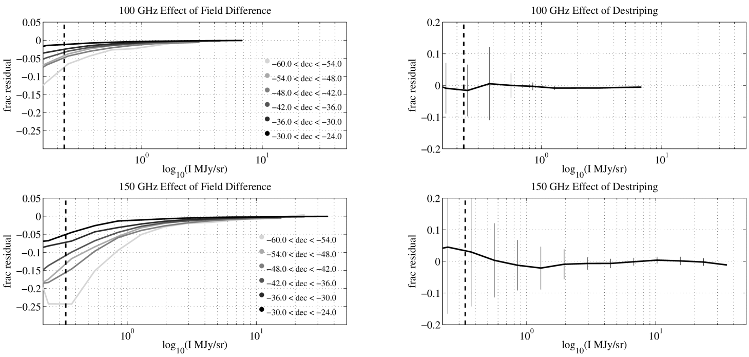
Figure 14.— Effect of field differencing and destriping on map pixel values, for FDS model 8 signal-only simulations. Top and bottom are 100 GHz and 150 GHz respectively. Left: Mean fractional change in pixel values of $m_{0}$ map, before and after field differencing, as a function of input pixel value. Lines in different shades of gray correspond to different bins in dec, as denoted in the legend. Right: Mean fractional change in pixel values before and after destriping process (i.e. comparing $m_{1}$ and $m_{2}$ maps). The error bars correspond to the standard deviation in each bin in $\log_{10}I~{}\mathrm{(MJy/sr)}$.

A.4. Fourier Plane Interpretation of Map Destriping Algorithm

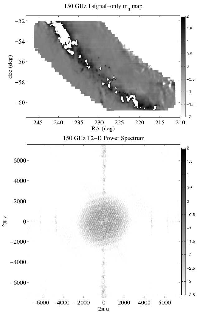
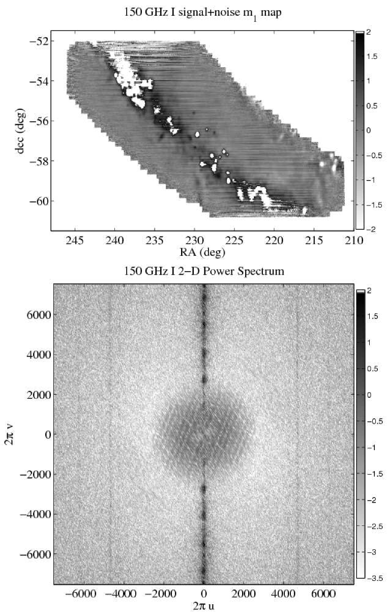
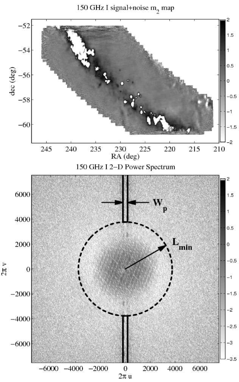
Figure 15.— Demonstration of Fourier plane interpretation of destriping process using FDS model 8 simulations. In each column, the 150 GHz I map (top; colorscale in MJy/sr with saturated pixels within survey region in white) and corresponding 2D auto power spectrum $C_{\bf{u}}$ (bottom) are shown for part of the fourth quadrant data. Note that in the power spectrum plots, the color scale is the same for each panel, and is logarithmic. Left: DC-level+slope filtered map $m_{0}$ using a signal-only simulation. In the power spectrum, vertical bands are an unavoidable consequence of our scan strategy. Center: same as Left, for a signal+noise simulation. The $1/f$ noise, which is added in the scan direction, is obvious as the increase in power in the vertical band. Right: Equivalent plots for the destriped map and $C_{\bf{u}}$ — there is a large reduction in the $1/f$ noise in the destriped map, and no obvious residuals have been introduced due to the choice of $n_{p}$ and $L_{min}$. In the power spectrum plot, we show the interpretation of the trench dug by the polynomial filter of order $n_{p}$ on the timestream; $L_{min}$ indicates the width of $\tilde{K}$, i.e. the angular scale below which modes are preserved. Modes inside the circle are subtracted from the timestream, as in Equation A1.

Experiments such as QUaD which use fixed elevation scans suffer $1/f$ noise predominantly in the scan direction. The $1/f$ noise appears as a vertical band in the two-dimensional power spectrum $C_{\bf{u}}=\tilde{I}\left(\bf{u}\right)\tilde{I}\left(\bf{u}\right)^{*}$, where $\tilde{I}$ is the Fourier transform of the total intensity map, and ${\bf{u}}=\left(u,v\right)$ is the wavevector. The leftmost panels of Figure 15 show a signal-only map and $C_{\bf{u}}$ from an FDS simulation of a subsection of the survey; an example signal+noise $m_{0}$ map and corresponding $C_{\bf{u}}$ are displayed in the center panels, where the vertical noise band is clearly visible in the 2D power spectrum. Polynomial filtering over the entirety of each scan digs a ‘trench’ into the signal and noise in the vertical band: the width of the trench in Fourier space, $W_{p}$, is determined by the polynomial order $n_{p}$, i.e. $W_{p}\propto n_{p}$.

In the destriping method, we interpolate ‘signal-only’ data from the template map $m_{t}$ to remove large-scale (low $|\bf{u}|$) modes before filtering, or equivalently removing modes inside the circle in the center panel of Figure 15. The smallest mode removed is $L_{min}$ — the width of the Fourier transform of the smoothing kernel, $\tilde{K}(\bf{u})$, used to generate the template signal map $m_{t}$. With the low-$|\bf{u}|$ modes removed, instead of digging a trench along the entire vertical band in the Fourier Plane, as in the usual case of polynomial filtering, we filter the same width trench $W_{p}$, but only for modes with $|\bf{u}|>L_{min}$. Residuals from filtering bright point sources (which dominate the signal at large $\bf{u}$) can be avoided by masking the brightest sources during the polynomial filtering in Equation A2.

The lower right panel of Figure 15 demonstrates the result when applying the destriping method with a 6th order polynomial — filtering has removed much of the noise along the vertical axis. The corresponding map (top right panel) shows that $1/f$ noise has been heavily suppressed, without the introduction of obvious residuals. We note that some of the $1/f$ noise has been filtered inside $L_{min}$; this is due to the fact that $L_{min}$ is not in fact a hard boundary in Fourier space, but rather the width of $\tilde{K}$, which in the present case is a gaussian function. Smoothing therefore allows filtering of different modes with $\bf{u}$-dependent ‘weighting’, with the weight equal to $\tilde{K}$ evaluated at each $\bf{u}$.

The plots indicate that though the algorithm is implemented entirely in map/timestream space, its effect is equivalent to a Fourier plane filter. Tests on simulated data demonstrate that if uniform scan weighting is used, the algorithm is precisely linear in nature.

Appendix B Effect of Filtering and Map Processing on Diffuse Properties

In the following sections, the recovery of diffuse properties is tested with signal-only simulations, binned into the same coarse-resolution pixels used for analysis of the QUaD data. When comparing input to output values, Equation 4 is minimized as with the real data, except that no error bars are present because signal-only simulations are used. All uncertainties quoted in this section therefore reflect the scatter introduced by processing effects, and are quantified by the intrinsic scatter term of Equation 4.

B.1. Total Intensity Spectral Index

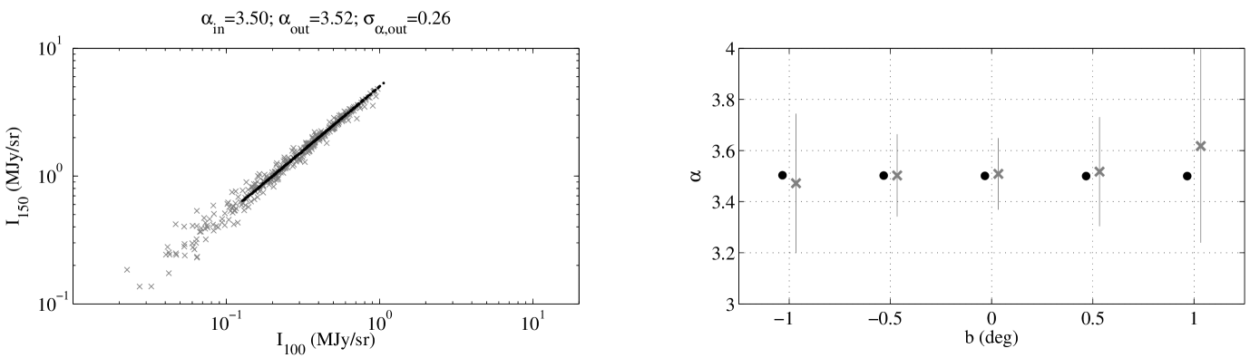
Figure 16.— Signal-only simulations of spectral index recovery. Left: Scatter plot showing input pixel values (black) and those after filtering, field-differencing, and destriping (gray crosses). The input and output mean spectral index $\alpha$ is shown above the plot, with the intrinsic scatter introduced by processing effects. Right: Spectral index as a function of galactic latitude $b$. Mean input is shown as black points, recovered is gray, with error bars indicating the intrinsic scatter in each $b$ bin.

To test the recovery of the spectral index, a signal-only simulation of the FDS dust model 8 is generated, with the model evaluated at the central frequency of each QUaD band as quoted in Section 4.3. The simulated timestreams are passed through the mapmaking code in exactly the same way as the real data, thus incorporating the effects of field-differencing and filtering.

Note that the $m_{2}$ mapmaking stage requires source detection and masking, but signal-to-noise thresholds cannot be used to determine the location of bright sources with signal only simulations. To circumvent this problem, signal plus noise simulations of the same simulated input maps are generated, with the corresponding $m_{1}$ maps used to determine the locations of sources to be masked. The resulting source catalog is then used in the $m_{2}$ mapmaking stage of the signal-only simulations to reproduce the effects of the filtering strategy on signal-only data.

The input average spectral index was found to be $\alpha=3.5$, with a recovered value of $\alpha=3.52$ and intrinsic scatter $\sigma_{\alpha}=0.26$, with the scatter introduced by the data processing and mapmaking steps. The left panel of Figure 16 shows the input and recovered pixel values of $I_{150}$ against $I_{100}$, while the right panel shows the input and recovered $\alpha$ as a function of $b$. Both panels show that the input spectral index is recovered to within the scatter introduced by the data processing, with a small systematic defecit of $<1\%$ in $\alpha$.

B.2. Polarization

The effects of field-differencing and filtering on the recovery of the polarization fraction are investigated by using two signal-only simulations, again with FDS dust model 8 as the input total intensity, but using assumed polarization fractions of 2 and 5%, with the polarization signal purely $+Q$ (in galactic coordinates). From these maps, we simulate QUaD observations and pass the resulting timestream through the mapmaking algorithm as in B.

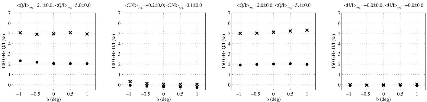
Figure 17.— Signal only simulations of galactic-longitude averaged polarization fraction, as a function of galactic latitude. From left to right: 100 GHz $Q/I$ and $U/I$, 150 GHz  $Q/I$ and $U/I$. Crosses (dots) correspond to assumed 5 (2)% polarization fraction simulations. All input polarized signal is in $+Q$ in galactic coordinates, with $U=0$ everywhere. The average recovered values of the polarization fraction are shown above each plot, with the ‘error’ representing the intrinsic scatter introduced by data processing and mapmaking; in the plots of polarization fraction in bins of $b$, this quantity is shown as an error bar.

Figure 17 demonstrates that for both 2% and 5% simulations, the input polarization fraction is recovered without introducing any strong systematic bias. Fluctuations in polarization fraction due to filtering and map processing effects are $0.1$–$0.2$%, and thus introduce a small error on the average polarization fraction measured by QUaD, though such systematic effects do influence the recovery of polarization angle.

Figure 18 shows the recovery of polarization angle from the same simulations. Similarly to polarization fraction, the input polarization angle is recovered to within 1$\sigma$ of the introduced scatter, both as an average, and within individual bins of galactic latitude. From the average over all pixels, the fluctuation in $\phi$ due to processing and filtering the simulated data at 100 GHz is $17.1^{\circ}$ for 5% polarization fraction, or $26.5^{\circ}$ for 2% polarization fraction. At 150 GHz, we find $3.2^{\circ}$ ($13.1^{\circ}$) for 5% (2%). The systematic shift of recovered polarization angle is $\sim 5^{\circ}$ ($\sim 2^{\circ}$) for the 2% polarization fraction simulations at 100 (150 GHz), and $\sim 0.2^{\circ}$ ($\sim 0.4^{\circ}$) for the 5% polarization fraction simulations at at 100 (150 GHz). We conservatively adopt the larger of these quantities when estimating systematic errors, i.e. the systematic error on the average recovered $\phi$ is $5^{\circ}$ at 100 GHz and $2^{\circ}$ at 150 GHz.

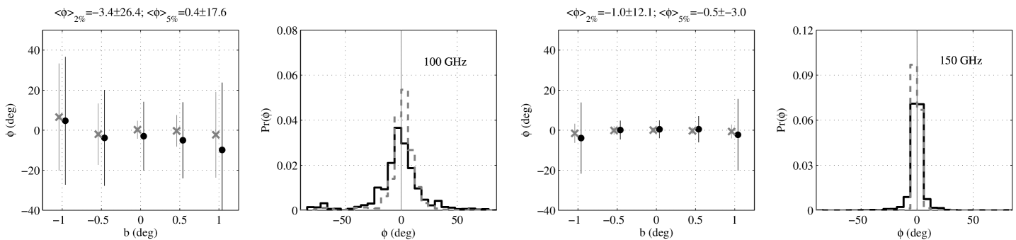
Figure 18.— Signal-only simulations of polarization angle $\phi$: The left two panels are 100 GHz $\phi$ vs $b$, and the probability distribution of the pixel values as a function of $\phi$. In the former, the error bars indicate the level of intrinsic scatter introduced by processing effects. Gray crosses (black dots) are for the 5 (2)% polarization fraction simulations. The numbers above the plots are the average polarization angles in each $b$ bin, with the ‘error’ indicating the average intrinsic scatter due to data processing. In the probability plots, the gray vertical line shows the input $\phi=0^{\circ}$; gray broken (black solid) lines are for the 5 (2)% polarization fraction simulations. The right two panels are the same for 150 GHz.

Appendix C Celestial Coordinate Maps

Figures 19–21 show the celestial coordinate $m_{2}$ maps.

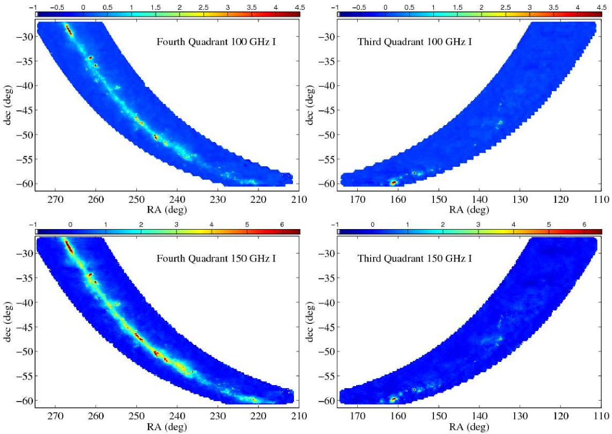
Figure 19.— I maps for fourth quadrant (left column) and third quadrant (right column), at 100 GHz (top row) and 150 GHz (bottom row). The color scale is MJy/sr.

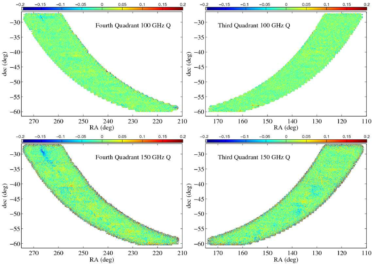
Figure 20.— Q maps for fourth quadrant (left column) and third quadrant (right column), at 100 GHz (top row) and 150 GHz (bottom row). The color scale is MJy/sr.

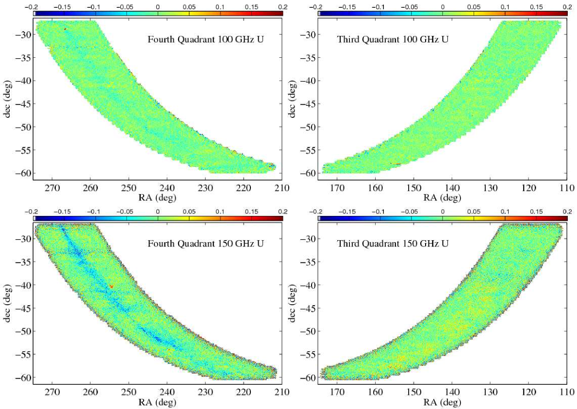
Figure 21.— U maps for fourth quadrant (left column) and third quadrant (right column), at 100 GHz (top row) and 150 GHz (bottom row). The color scale is MJy/sr.

References

- Ade et al. (2008) Ade, P. et al. 2008, ApJ, 674, 22
- Bennett et al. (1994) Bennett, C. L. et al. 1994, ApJ, 434, 587
- Benoît et al. (2004) Benoît, A. et al. 2004, A&A, 424, 571
- Bertin & Arnouts (1996) Bertin, E., & Arnouts, S. 1996, A&AS, 117, 393
- Brown et al. (2009) Brown, M. L. et al. 2009, ApJ, 705, 978
- Comito et al. (2005) Comito, C., Schilke, P., Phillips, T. G., Lis, D. C., Motte, F., & Mehringer, D. 2005, ApJS, 156, 127
- Dame et al. (2001) Dame, T. M., Hartmann, D., & Thaddeus, P. 2001, ApJ, 547, 792
- Dunkley et al. (2009) Dunkley, J. et al. 2009, in American Institute of Physics Conference Series, Vol. 1141, American Institute of Physics Conference Series, ed. S. Dodelson, D. Baumann, A. Cooray, J. Dunkley, A. Fraisse, M. G. Jackson, A. Kogut, L. Krauss, M. Zaldarriaga, & K. Smith , 222–264
- Finkbeiner (2001) Finkbeiner, D. P. 2001, private communication
- Finkbeiner (2003) ——. 2003, ApJS, 146, 407
- Finkbeiner et al. (1999) Finkbeiner, D. P., Davis, M., & Schlegel, D. J. 1999, ApJ, 524, 867
- Fixsen et al. (1999) Fixsen, D. J., Bennett, C. L., & Mather, J. C. 1999, ApJ, 526, 207
- Gold et al. (2009) Gold, B. et al. 2009, ApJS, 180, 265
- Groesbeck (1995) Groesbeck, T. D. 1995, PhD thesis, AA(California Institute Of Technology.)
- Hamaker & Bregman (1996) Hamaker, J. P., & Bregman, J. D. 1996, A&AS, 117, 161
- Haslam et al. (1981) Haslam, C. G. T., Klein, U., Salter, C. J., Stoffel, H., Wilson, W. E., Cleary, M. N., Cooke, D. J., & Thomasson, P. 1981, A&A, 100, 209
- Haslam et al. (1982) Haslam, C. G. T., Salter, C. J., Stoffel, H., & Wilson, W. E. 1982, A&AS, 47, 1
- Heiles (1996) Heiles, C. 1996, ApJ, 462, 316
- Hildebrand et al. (2000) Hildebrand, R. H., Davidson, J. A., Dotson, J. L., Dowell, C. D., Novak, G., & Vaillancourt, J. E. 2000, PASP, 112, 1215
- Hinderks et al. (2009) Hinderks, J. et al. 2009, ApJ, 692, 1221
- Hinshaw et al. (2009) Hinshaw, G. et al. 2009, ApJS, 180, 225
- Hu & White (1997) Hu, W., & White, M. 1997, New Astronomy, 2, 323
- Jones et al. (2003) Jones, W. C., Bhatia, R., Bock, J. J., & Lange, A. E. 2003, in Presented at the Society of Photo-Optical Instrumentation Engineers (SPIE) Conference, Vol. 4855, Millimeter and Submillimeter Detectors for Astronomy. Edited by Phillips, Thomas G.; Zmuidzinas, Jonas. Proceedings of the SPIE, Volume 4855, pp. 227-238 (2003)., ed. T. G. Phillips & J. Zmuidzinas, 227–238
- Kogut et al. (2007) Kogut, A. et al. 2007, ApJ, 665, 355
- Lazarian (2003) Lazarian, A. 2003, Journal of Quantitative Spectroscopy and Radiative Transfer, 79, 881
- Leitch et al. (2002) Leitch, E. M. et al. 2002, ApJ, 568, 28
- Masi et al. (2006) Masi, S. et al. 2006, A&A, 458, 687
- Netterfield et al. (2009) Netterfield, C. B. et al. 2009, ArXiv e-prints, 0904.1207
- Nummelin et al. (1998) Nummelin, A., Bergman, P., Hjalmarson, A., Friberg, P., Irvine, W. M., Millar, T. J., Ohishi, M., & Saito, S. 1998, ApJS, 117, 427
- Olmi et al. (2009) Olmi, L. et al. 2009, ArXiv e-prints, 0910.1097
- Ponthieu et al. (2005) Ponthieu, N. et al. 2005, A&A, 444, 327
- Prunet et al. (1998) Prunet, S., Sethi, S. K., Bouchet, F. R., & Miville-Deschenes, M. 1998, A&A, 339, 187
- Pryke et al. (2009) Pryke, C. et al. 2009, ApJ, 692, 1247
- Schäfer et al. (2006) Schäfer, B. M., Pfrommer, C., Hell, R. M., & Bartelmann, M. 2006, MNRAS, 370, 1713
- Schuller et al. (2009) Schuller, F. et al. 2009, A&A, 504, 415
- Valls-Gabaud (1998) Valls-Gabaud, D. 1998, Publications of the Astronomical Society of Australia, 15, 111
- Villa et al. (2002) Villa, F. et al. 2002, in American Institute of Physics Conference Series, Vol. 616, Experimental Cosmology at Millimetre Wavelengths, ed. M. de Petris & M. Gervasi, 224–228
- Weiner et al. (2006) Weiner, B. J. et al. 2006, ApJ, 653, 1049
- Wright et al. (1991) Wright, E. L. et al. 1991, ApJ, 381, 200
- Wyrowski et al. (2006) Wyrowski, F., Heyminck, S., Güsten, R., & Menten, K. M. 2006, A&A, 454, L95
- Zweibel & Heiles (1997) Zweibel, E. G., & Heiles, C. 1997, Nature, 385, 131