Fully selfconsistent GW calculations for molecules

Abstract

We calculate single-particle excitation energies for a series of 33 molecules using fully selfconsistent GW, one-shot G₀W₀, Hartree-Fock (HF), and hybrid density functional theory (DFT). All calculations are performed within the projector augmented wave (PAW) method using a basis set of Wannier functions augmented by numerical atomic orbitals. The GW self-energy is calculated on the real frequency axis including its full frequency dependence and off-diagonal matrix elements. The mean absolute error of the ionization potential (IP) with respect to experiment is found to be 4.4, 2.6, 0.8, 0.4, and 0.5 eV for DFT-PBE, DFT-PBE0, HF, G₀W₀[HF], and selfconsistent GW, respectively. This shows that although electronic screening is weak in molecular systems its inclusion at the GW level reduces the error in the IP by up to 50% relative to unscreened HF. In general GW overscreens the HF energies leading to underestimation of the IPs. The best IPs are obtained from one-shot G₀W₀ calculations based on HF since this reduces the overscreening. Finally, we find that the inclusion of core-valence exchange is important and can affect the excitation energies by as much as 1 eV.

I Introduction

Density functional theory (DFT)hohenbergkohn with the single-particle Kohn-Sham (KS) schemekohnsham is today the most widely used approach to the electronic structure problem of real materials in both solid state physics and quantum chemistry. While properties derived from total energies (or rather total energy differences) are accurately predicted by DFT, it is well known that DFT suffers from a band gap problem implying that the single-particle KS eigenvalues cannot in general be interpreted as real quasiparticle (QP) excitation energies. In particular, semilocal exchange-correlation functionals severely underestimate the fundamental gap of both insulators, semi-conductors, and molecules.hybertsen86 ; perdew_zunger ; paier06 ; heyd05

The hybridbecke ; LYP ; pbe0 and screened hybridhse03 functionals, which admix around 25$\%$ of the (screened) Fock exchange with the local DFT exchange, generally improve the description of band gaps in bulk semi-conductors and insulatorspaier06 ; heyd05 . However, the orbital energies obtained for finite systems using such functionals still underestimate the fundamental gap, $I_{p}-E_{a}$, (the difference between ionization potential and electron affinity) by up to several electron volts. In fact, for molecules the pure Hartree-Fock (HF) eigenvalues are usually closer to the true electron addition/removal energies than are the hybrid DFT eigenvalues. This is because HF is self-interaction free and because screening of the exchange interaction is a relatively weak effect in molecular systems.perdew_zunger ; pemmaraju07 ; jarnak_comment . On the other hand, in extended systems the effect of self-interaction is less important and the long range Coulomb interaction becomes short ranged due to dynamical screening. As a consequence HF breaks down in extended systems leading to dramatically overestimated band gaps and a qualitatively incorret description of metals.hf_band_polyacethylene ; grosso ; hf_gap_Ar

The many-body GW approximation of Hedinhedin has been widely and succesfully used to calculate QP band structures in metals, semi-conductors, and insulators.hybertsen86 ; gunnarsson ; wilkins ; orr The GW approximation can be viewed as HF with a dynamically screened Coulomb interaction. The fact that the screening is determined by the system itself instead of being fixed a priori as in the screened hybrid schemes, suggests that the GW method should be applicable to a broad class of systems ranging from metals with strong screening to molecules with weak screening. With the entry of nanoscience the use of GW has been extended to low-dimensional systems and nanostructuresstan_eulett ; grossman01 ; hahn ; tb_dft ; louie ; reining ; Chelikowsky ; neaton ; thygesen09 ; Freysoldt ; juanma_prb and more recently even nonequilibrium phenomena like quantum transportthygesen_jcp ; thygesen_prl ; leeuwen_trans ; spataru2 ; verdozzi . In view of this trend it is important to establish the performance of the GW approximation for other systems than the crystalline solids. In this work we present first-principles benchmark GW calculations for a series of small molecules. In a closely related study we compared GW and Hartree-Fock to exact diagonalization results for semi-empirical PPP models of conjugated moleculespaperI . The main conclusions from the two studies regarding the qualities of the GW approximation in molecular systems, are very consistent.

Most GW calculations to date rely on one or several approximations of more technical character. These include the plasmon pole approximation, the linearized QP equation, neglect of off-diagonal matrix elements in the GW self-energy, analytic continuations from the imaginary to the real frequency axis, neglect of core states contributions to the self-energy, neglect of self-consistency. The range of validity of these approximations has been explored for solid state systems by a number of authorsbarth ; usuda_hamada ; ku ; schilfgaarde_prb ; Shishkin2006 ; rinke , however, much less is known about their applicability to molecular systemsstan_eulett . Our implementation of the GW method avoids all of these technical approximations allowing for a direct and unbiased assessment of the GW approximation itself.

Here we report on single-shot G₀W₀ and fully self-consistent GW calculations of QP energies for a set of 33 molecules. The calculated IPs are compared with experimental values as well as single-particle eigenvalues obtained from Hartree-Fock and DFT-PBE/PBE0 theories. As additional benchmarks we compare to second-order Möller-Plesset (MP2) and DFT-PBE total energy differences between the neutral and cation species. Special attention is paid to the effect of selfconsistency in the GW self-energy and the role of the initial Green function, $G_{0}$, used in one-shot G₀W₀ calculations. The use of PAW rather than pseudopotentials facilitate the inclusion of core-valence exchange, which we find can contribute significantly to the HF and GW energies. Our results show that the GW approximation yields accurate single-particle excitation energies for small molecules improving both hybrid DFT and full Hartree-Fock results.

The paper is organized as follows. In Sec. II we describe the theoretical and numerical details behind the GW calculations, including the augmented Wannier function basis set, the self-consistent solution of the Dyson equation, and the evaluation of valence-core exchange within PAW. In Sec. III we discuss and compare the results of G₀W₀, GW, HF, PBE0, and PBE calculations. We analyze the role of dynamical screening, and discuss the effect of self-consistency in the GW self-energy. We conclude in Sec. IV.

II Method

II.1 Augmented Wannier function basis

For the GW calculations we apply a basis set consisting of projected Wannier functions (PWF) augmented by numerical atomic orbitals (NAO). The PWFs, $\phi_{i}$, are obtained by maximizing their projections onto a set of target NAOs, $\Phi_{Alm}$, subject to the condition that they span the set of occupied eigenstates, $\psi_{n}$. Thus we maximize the functional

$$\Omega=\sum_{i}\sum_{A,l,m}|\langle\phi_{i}|\Phi_{Alm}\rangle|^{2}$$ (1)

subject to the condition $\text{span}\{\phi_{i}\}\supseteq\text{span}\{\psi_{n}\}_{\text{occ}}$ as described in Ref. quambo, . The target NAOs are given by $\Phi_{Alm}(\mathbb{r})=\zeta_{Al}(r)Y_{lm}(\mathbb{r})$ where $\zeta_{Al}$ is a modified Gaussian which vanish outside a specified cut-off radius, and $Y_{lm}$ are the spherical harmonics corresponding to the valence of atom $A$. The number of PWFs equals the number of target NAOs. For example we obtain one PWF for H ($l_{\text{max}}=0$), and four PWFs for C ($l_{\text{max}}=1$). The PWFs mimick the target atomic orbitals but in addition they allow for an exact representation of all the occupied molecular eigenstates. The latter are obtained from an accurate real-space PAW-PBE calculationGPAW ; GPAW-LCAO .

The PWFs obtained in this way provide an exact representation of the occupied PBE eigenstates. However, this does not suffice for GW calculations because the polarizability, $P$, and the screened interaction, $W$, do not live in this subspace. Hence we augment the PWFs by additional NAOs including so-called polarization functions which have $l=l_{\text{max}}+1$ and/or extra radial functions (zeta functions) for the valence atomic orbitals. For more details on the definition of polarization- and higher zeta functions we refer to Ref. GPAW-LCAO, . To give an example, a double-zeta-polarized (DZP) basis consists of the PWFs augmented by one set of NAOs corresponding to $l=0,...,l_{\text{max}}$ and one set of polarization orbitals. Note that the notation, SZ, SZP, DZ, DZP, etc., is normally used for pure NAO basis sets, but here we use it to denote our augmented Wannier basis set. We find that the augmented Wannier basis is significantly better for HF and GW calculations than the corresponding pure NAO basis.

The GW and HF calculations presented in Sec. III were performed using a DZP augmented Wannier basis. This gives a total of 5 basis functions per H, Li, and Na, and 13 basis functions for all other chemical elements considered. In Sec. III.3 we discuss convergence of the GW calculations with respect to the size of the augmented Wannier basis.

II.2 GW calculations

The HF and GW calculations for isolated molecules are performed using a Green function code developed for quantum transport.thygesen_gw_prb In principle, this scheme is designed for a molecule connected to two electrodes with different chemical potentials $\mu_{L}$ and $\mu_{R}$. However, the case of an isolated molecule can be treated as a special case by setting $\mu_{L}=\mu_{R}=\mu$ and modelling the coupling to electrodes by a constant imaginary self-energy, $\Sigma_{L/R}=i\eta$. The chemical potential $\mu$ is chosen to lie in the HOMO-LUMO gap of the molecule and the size of $\eta$, which provides an artifical broadening of the discrete levels, is reduced until the results have converged. In this limit of small $\eta$ the result of the GW calculation becomes independent of the precise position of $\mu$ inside the gap.

In Ref. thygesen_gw_prb, the GW-transport scheme was described for the case of an orthogonal basis set and for a truncated, two-index Coulomb interaction. Below we generalize the relevant equations to the case of a non-orthogonal basis and a full four-index Coulomb interaction. Some central results of many-body perturbation theory in a non-orthogonal basis can be found in Ref. nonorthogonal, .

The central object is the retarded Green function, $G^{r}$,

$$G^{r}(\varepsilon)=[(\varepsilon+i\eta)S-H_{\text{KS}}+v_{\text{xc}}-\Delta v_{\text{H}}-\Sigma_{\text{xc}}^{r}[G](\varepsilon)]^{-1}$$ (2)

In this equation all quantities are matrices in the augmented Wannier basis, e.g. $H_{\text{KS},ij}=\langle\phi_{i}|\hat{H}_{\text{KS}}|\phi_{j}\rangle$ is the KS Hamiltonian matrix and $S_{ij}=\langle\phi_{i}|\phi_{j}\rangle$ is an overlap matrix. The term $\Delta v_{\text{H}}$ represents the change in the Hartree potential relative to the DFT Hartree potential already contained in $H_{\text{KS}}$, see Appendix A. The local xc-potential, $v_{\text{xc}}$, is subtracted to avoid double counting when adding the many-body self-energy, $\Sigma_{\text{xc}}[G]$. As indicated, the latter depends on the Green function and therefore Eq. (2) must in principle be solved self-consistently in conjuction with the self-energy.

In the present study $\Sigma_{\text{xc}}$ is either the bare exchange potential or the GW self-energy. To be consistent with the code used for the calculations, we present the equations for the GW self-energy on the so-called Keldysh contour. However, under the equilibrium conditions considered here the Keldysh formalism is equivalent to the ordinary time-ordered formalism.

The GW self-energy is defined by

$$\Sigma^{\text{GW}}_{ij}(\tau,\tau^{\prime})=i\sum_{kl}G_{kl}(\tau,\tau^{\prime+})W_{ik,jl}(\tau,\tau^{\prime}),$$ (3)

where $\tau$ and $\tau^{\prime}$ are times on the Keldysh contour, $\mathcal{C}$. The dynamically screened Coulomb interaction obeys the Dyson-like equation

$$W_{ij,kl}(\tau,\tau^{\prime})=V_{ij,kl}\delta_{\mathcal{C}}(\tau,\tau^{\prime})\\ +\sum_{pqrs}\int_{\mathcal{C}}\!\mathrm{d}\tau_{1}V_{ij,pq}P_{pq,rs}(\tau,\tau_{1})W_{rs,kl}(\tau_{1},\tau^{\prime}),$$ (4)

and the polarization bubble is given by

$$P_{ij,kl}(\tau,\tau^{\prime})=-iG_{ik}(\tau,\tau^{\prime})G_{lj}(\tau^{\prime},\tau).$$ (5)

In the limit of vanishing polarization, $P=0$, $W$ reduces to the bare Coulomb interaction

$$V_{ij,kl}=\iint\!\frac{\mathrm{d}\bm{r}\,\mathrm{d}\bm{r}^{\prime}}{|\bm{r}-\bm{r}^{\prime}|}\phi_{i}(\bm{r})\phi^{*}_{j}(\bm{r})\phi_{k}^{*}(\bm{r}^{\prime})\phi_{l}(\bm{r}^{\prime})$$ (6)

and the GW self-energy reduces to the exchange potential of HF theory.

From the above equations for the contour-ordered quantities, the corresponding real time components, i.e. the retarded, advanced, lesser, and greater components, can be obtained from standard conversion ruleshaug_jauho ; leeuwen_keldysh . For completeness we give the expressions for the real time components of the GW equations in Appendix A.

The time/energy dependence of the dynamical quantities $G$, $W$, $P$, and $\Sigma$, is represented on a uniform grid. We switch between time and energy domains using the Fast Fourier Transform in order to avoid time consuming convolutions. A typical energy grid used for the GW calculations in this work ranges from -150 to 150 eV with a grid spacing of 0.02 eV. The code is parallelized over basis functions and energy grid points. We use a Pulay mixing scheme for updating the Green function $G^{r}$ when iterating Eq. (2) to self-consistency as described in Ref. thygesen_gw_prb, .

We stress that no approximation apart from the finite basis set is made in our implementation of the GW approximation. In particular the frequency dependence is treated exactly and analytic continuations from the imaginary axis are avoided since we work directly on the real frequency/time axis. The price we pay for this is the large size of the energy grid.

II.3 Spectral function

The single-particle excitation spectrum is contained in the spectral function

$$A(\varepsilon)=i(G^{r}(\varepsilon)-[G^{r}(\varepsilon)]^{\dagger}).$$ (7)

For a molecule $A(\varepsilon)$ shows peaks at the QP energies $\varepsilon_{n}=E_{n}(N+1)-E_{0}(N)$ and $\varepsilon_{n}=E_{0}(N)-E_{n}(N-1)$ corresponding to electron addition and removal energies, respectively. Here $E_{n}(N)$ denotes the energy of the $n$th excited state of the system with $N$ electrons and $N$ refers to the neutral state.

When the Green function is evaluated in a non-orthogonal basis, like the augmented Wannier basis used here, the projected density of states for orbital $\phi_{i}$ becomes

$$D_{i}(\varepsilon)=[SA(\varepsilon)S]_{ii}~{}/~{}2\pi S_{ii},$$ (8)

where matrix multiplication is implied.nonorthogonal Correspondingly, the total density of states, or quasiparticle spectrum, is given by

$$D(\varepsilon)=\operatorname{Tr}(A(\varepsilon)S)/2\pi.$$ (9)

II.4 Calculating Coulomb matrix elements

The calculation of all of the Coulomb matrix elements, $V_{ij,kl}$, is prohibitively costly for larger basis sets. Fortunately the matrix is to a large degree dominated by negligible elements. To systematically define the most significant Coulomb elements, we use the product basis technique of Aryasetiawan and Gunnarsson aryasetiawan ; stan_levels . In this approach, the pair orbital overlap matrix

$$S_{ij,kl}=\langle n_{ij}|n_{kl}\rangle,$$ (10)

where $n_{ij}(\mathbb{r})=\phi_{i}^{*}(\mathbb{r})\phi_{j}(\mathbb{r})$ is used to screen for the significant elements of $V$.

The eigenvectors of the overlap matrix Eq. (10) represents a set of “optimized pair orbitals” and the eigenvalues their norm. Optimized pair orbitals with insignificant norm must also yield a reduced contribution to the Coulomb matrix, and are omitted in the calculation of $V$. We limit the basis for $V$ to optimized pair orbitals with a norm larger than $10^{-5}a_{0}^{-3}$. This gives a significant reduction in the number of Coulomb elements that needs to be evaluated, and it reduces the matrix size of $P(\varepsilon)$ and $W(\varepsilon)$ correspondingly, see Appendix A.

The evaluation of the double integral in Eq. (6) is efficiently performed in real space by solving a Poisson equation using multigrid techniquesGPAW ; Walter2008 .

II.5 Valence-core exchange

All inputs to the GW/HF calculations, i.e. the selfconsistent Kohn-Sham Hamiltonian, $H_{\text{KS}}$, the xc potential $v_{\text{xc}}$, the Coulomb matrix elements, $V_{ij,kl}$, are calculated using the real-space PAWbloechl code GPAWGPAW ; GPAW-LCAO .

In GPAW, the core electrons (which are treated scalar-relativistically) are frozen into the orbitals of the free atoms, and the Kohn-Sham equations are solved for the valence states only. Unlike pseudo potential schemes, these valence states are subject to the full potential of the nuclei and core electrons. This is achieved by a partitioning scheme, where quantities are divided into pseudo components augmented by atomic corrections. The operators obtained from GPAW are thus full-potential quantities, and the wave functions from which the Wannier basis functions are constructed correspond to the all-electron valence states. Ref. Walter2008, describes how the all-electron Coulomb elements can be determined within the PAW formalism.

Since both core and all-electron valence states are available in the PAW method, we can evaluate the contribution to the valence exchange self-energy coming from the core electrons. As the density matrix is simply the identity matrix in the subspace of atomic core states, this valence-core exchange reads

$$\Sigma_{x,ij}^{\text{core}}=-\sum_{k}^{\text{core}}V_{ik,jk},$$ (11)

where $i,j$ represent valence basis functions. We limit the inclusion of valence-core interactions to the exchange potential, neglecting it in the correlation. This is reasonable, because the polarization bubble, $P$, involving core and valence states will be small due to the large energy difference and small spatial overlap of the valence and core states. This procedure was used and validated for solids in Ref. Shishkin2006, . We find that the elements of $\Sigma_{x,ij}^{\text{core}}$ can be significant – on average 1.2 eV for the HOMO – and are larger (more negative) for the more bound orbitals which have larger overlap with the core states. In general, the effect on the HOMO-LUMO gap is to enlarge it, on average by 0.4 eV because the more bound HOMO level is pushed further down than the less bound LUMO state. In the case of solids, the role of valence-core interaction has been investigated by a number of authorsusuda_hamada ; ku ; schilfgaarde_prb ; Shishkin2006 ; engel . Here the effect on the QP band gap seems to be smaller than what we find for the molecular gaps. We note that most GW calculations rely on pseudopotential schemes where these valence-core interactions are not accessible. In such codes, the xc contribution from the core electrons are sometimes estimated by $\Sigma^{\text{core}}_{\text{xc}}\approx v_{\text{xc}}[n]-v_{\text{xc}}[n_{\text{val}}]$ where $n_{\text{val}}$ is the valence electron density, but as the local xc potential is a non-linear functional of the density, this procedure is not well justified. Instead we subtract the xc potential of the full electon density $n$, and add explicitly the exact exchange core contribution.

III Results

In Fig. 1 we compare the calculated HOMO energies with experimental ionization potentials for the 33 molecules listed in Table 1. The geometries of the molecules, which all belong to the G2 test set, are taken from Ref. geom, . The different HOMO energies correspond to: DFT-PBEpbe and DFT-PBE0pbe0 eigenvalues, Hartree-Fock eigenvalues, and fully selfconsistent GW. The GW energies are obtained from the peaks in the corresponding density of states Eq. (9) extrapolated to $\eta=0$ ($\eta$ gives an artificial broadening of the delta peaks).

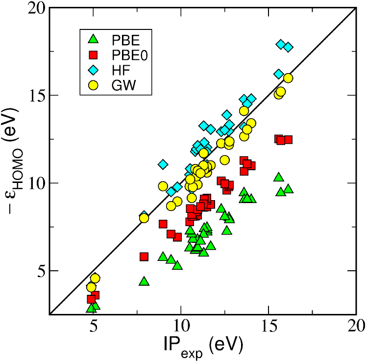
Figure 1: (Color online) Calculated negative HOMO energy versus experimental ionization potential. Both PBE and PBE0 systematically understimates the ionization energy due to self-interaction errors while HF overestimates it slightly. The dynamical screening from the GW correlation lowers the HF energies bringing them closer to the experimental values. Numerical values are listed in Table 1.

We stress the different meaning of fully selfconsistent GW and the recently introduced method of quasiparticle selfconsistent GWschilfgaarde_qsGW : In fully selfconsistent GW the Green function obtained from Dyson’s equation Eq. (2) with $\Sigma_{xc}[G]=\Sigma_{\text{GW}}[G]$ is used to calculate the $\Sigma_{\text{GW}}$ of the next iteration. In QP-selfconsistent GW, $\Sigma_{\text{GW}}$ is always evaluated using a non-interacting Green function and the self-consistency is obtained when the difference between the non-interacting GF and the interacting GF, is minimal.

Fig. 1 clearly shows that both the PBE and PBE0 eigenvalues of the HOMO severely underestimates the ionization potential. The average deviation from the experimental values are 4.35 eV and 2.55 eV, respectively. The overestimation of the single-particle eigenvalues of occupied states is a well known problem of DFT and can be ascribed to the insufficient cancellation of the self-interaction in the Hartree potential.perdew_zunger ; pemmaraju07 Part of this self-interaction is removed in PBE0. However, the fact that the HF results are significantly closer to experiments indicates that the 25% Fock exchange included in the PBE0 is not sufficient to cure the erroneous description of (occupied) molecular orbitals. On the other hand PBE0 gives good results for band gaps in semi-conductors and insulators where in contrast full Hartree-Fock does not perform well.hf_band_polyacethylene ; grosso ; hf_gap_Ar We conclude that the amount of Fock exchange to be used in the hybrid functionals to achieve good quasiparticle energies is highly system dependent. A similar problem is encountered with self-interaction corrected exchange-correlation functionals.pemmaraju07

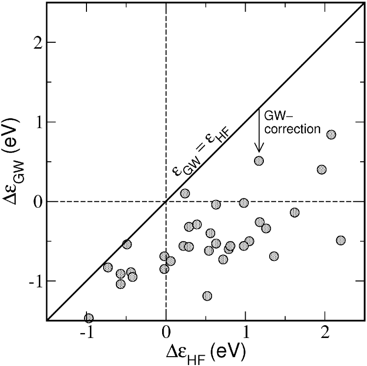
Figure 2: The deviation of the calculated HOMO energy from the experimental ionization potential in GW and HF, respectively. The vertical displacement of points from the line $x=y$ gives the difference between the GW and HF energies and represents the effect of screening. Notice that the GW correction is always negative (corresponding to higher HOMO energy) and that it generally overcorrects the HF energies. Also notice that the GW correction is larger for molecules where HF presents the largest overestimation of the ionization potential.

As can be seen from Fig. 1, GW performs better than Hartree-Fock for the HOMO energy yielding a mean absolute error with respect to experiments of 0.5 eV compared to 0.81 eV with Hartree-Fock. As expected the difference between HF and GW is not large on an absolute scale (around 1 eV on average, see Table 2) illustrating the fact that screening is weak in small molecules. On a relative scale selfconsistent GW improves the agreement with experiments by almost 30% as compared to HF.

To gain more insight into the influence of screening on the orbital energies, we compare in Fig. 2 the deviation of the HF and GW energies from $\text{IP}_{\text{exp}}$. The GW self-energy can be split into the bare exchange potential and an energy-dependent correlation part

$$\Sigma_{\text{GW}}(\bm{r},\bm{r}^{\prime};\varepsilon)=v_{x}(\bm{r},\bm{r}^{\prime})+\Sigma_{\text{corr}}(\bm{r},\bm{r}^{\prime};\varepsilon)$$ (12)

Accordingly the quasiparticle energy can be written as the bare HF energy and a correction due to the energy-dependent part of the GW self-energy (the dynamical screening term)

$$\varepsilon_{n}^{\text{QP}}=\varepsilon_{n}^{\text{HF}}+\Delta_{n}^{\text{GW}}.$$ (13)

In Fig. 2 the line $y=x$ corresponds to $\Delta_{n}^{\text{GW}}=0$, and the vertical displacement from the line thus represents the effect of screening on the calculated HOMO energy. We first notice that the effect of screening is to shift the HOMO level upwards in energy, i.e. to reduce the ionization potential. This can be understood by recalling that the Hartree-Fock eigenvalue represents the energy cost of removing an electron from the HOMO when orbital relaxations in the final state are neglected (Koopmans’ theoremgrosso ). In Ref. paperI, we showed, on the basis of GW and exact calculations for semi-empirical models of conjugated molecules, that $\Delta_{n}^{\text{GW}}$ mainly describes the orbital relaxations in the final state and to a lesser extent accounts for the correlation energy of the initial and final states. This explains the negative sign of $\Delta_{n}^{\text{GW}}$ because the inclusion of orbital relaxation in the final state lowers the energy cost of removing an electron. We note that this is different from the situation in extended, periodic systems where orbital relaxations vanish and the main effect of the GW self-energy is to account for correlations in the initial and final states.

Table 1: Experimental ionization potential (first column) and HOMO energy calculated using different approximations for exchange and correlation. “X-eig” refers to a single-particle eigenvalue while “X-tot” refers to a total energy difference, $E(N)-E(N-1)$. The G₀W₀(PBE) energies have been obtained from the QP equation while the GW and G₀W₀ energies are obtained from the DOS in Eq. (9). Last row shows the mean absolute error (MAE) with respect to experiments. All energies are in eV.

Molecule	Expt.(a)		PBE-eig		PBE0-eig		HF-eig		GW		G0W0(HF)		G0W0(PBE)-QP		MP2(a)		PBE-tot
LiH	7.	90	4.	34	5.	81	8.	14	8.	0(b)	8.	2(b)	8.	0	8.	20	8.	02
Li2	5.	11	2.	96	3.	62	4.	62	4.	6	4.	7	4.	4	4.	91	5.	09
LiF	11.	30	6.	00	8.	62	13.	26	11.	7	11.	2	12.	0	12.	64	11.	87
Na2	4.	89	2.	81	3.	38	4.	16	4.	1	4.	3	4.	7	4.	48	4.	97
NaCl	9.	80	5.	24	6.	92	9.	78	9.	0	9.	2	8.	8	9.	63	9.	37
CO	14.	01	9.	05	10.	98	14.	80	13.	4	14.	1	13.	9	15.	08	13.	88
CO2	13.	78	9.	08	11.	09	14.	50	13.	1	13.	3	13.	6	14.	71	13.	64
CS	11.	33	7.	40	9.	09	12.	31	10.	8	11.	7	11.	0	12.	58	11.	31
C2H2	11.	49	7.	20	8.	64	11.	05	10.	6	11.	1	11.	2	11.	04	11.	39
C2H4	10.	68	6.	79	8.	11	10.	11	9.	8	10.	4	9.	6	10.	18	10.	67
CH4	13.	60	9.	43	11.	29	14.	77	14.	1	14.	4	14.	4(c)	14.	82	14.	10
CH3Cl	11.	29	7.	08	8.	80	11.	68	11.	0	11.	4	11.	1	11.	90	11.	10
CH3OH	10.	96	6.	31	8.	49	12.	14	10.	7	10.	8	10.	5	12.	16	10.	72
CH3SH	9.	44	5.	60	7.	09	9.	50	8.	8	9.	0	8.	4	9.	73	9.	29
Cl2	11.	49	7.	32	9.	02	12.	03	10.	9	11.	3	11.	5	12.	37	11.	22
ClF	12.	77	7.	90	9.	88	13.	33	12.	4	12.	4	13.	0	13.	63	12.	48
F2	15.	70	9.	43	12.	42	17.	90	15.	2	15.	2	16.	2	18.	20	15.	39
HOCl	11.	12	6.	68	8.	66	11.	93	10.	6	10.	8	11.	0	12.	23	10.	95
HCl	12.	74	8.	02	9.	78	12.	96	12.	2	12.	5	12.	5	13.	02	12.	71
H2O2	11.	70	6.	38	8.	78	13.	06	11.	0	11.	1	11.	1	13.	00	11.	18
H2CO	10.	88	6.	28	8.	37	11.	93	10.	4	10.	5	10.	6	11.	97	10.	80
HCN	13.	61	9.	05	10.	67	13.	19	12.	7	13.	2	12.	4	13.	33	13.	67
HF	16.	12	9.	61	12.	47	17.	74	16.	0	15.	6	15.	7	17.	35	16.	27
H2O	12.	62	7.	24	9.	59	13.	88	12.	3	12.	1	11.	9(d)	13.	62	12.	88
NH3	10.	82	6.	16	8.	11	11.	80	10.	8	11.	0	10.	6	11.	57	11.	02
N2	15.	58	10.	28	12.	51	16.	21	15.	1	15.	7	15.	6	16.	41	15.	39
N2H4	8.	98	5.	75	7.	67	11.	06	9.	8	10.	1	9.	5	11.	07	9.	90
SH2	10.	50	6.	29	7.	79	10.	48	9.	8	10.	1	9.	9	10.	48	10.	38
SO2	12.	50	8.	08	9.	96	13.	02	11.	3	11.	7	11.	7	13.	46	12.	12
PH3	10.	95	6.	79	8.	17	10.	38	9.	9	10.	3	10.	0	10.	50	10.	39
P2	10.	62	7.	09	8.	21	9.	65	9.	2	9.	8	9.	0	10.	09	10.	37
SiH4	12.	30	8.	50	10.	13	12.	93	12.	3	12.	6	12.	4(e)	13.	25	11.	95
Si2H6	10.	53	7.	27	8.	54	10.	82	10.	2	10.	6	9.	9	11.	03	10.	36
SiO	11.	49	7.	46	9.	14	11.	78	10.	9	11.	2	11.	3	11.	82	11.	27
MAE	-		4.	35	2.	55	0.	81	0.	5	0.	4	0.	5	0.	82	0.	24

Table 2: Mean absolute deviation between the IPs of the 33 molecules calculated with the different methods and experiment. The mean absolute deviation with respect to experiment coincide with the last row in Table 1

Method	Expt.${}^{\text{(a)}}$		PBE-eig		PBE0-eig		HF-eig		GW		G0W0[HF]		MP2${}^{\text{(a)}}$		PBE-tot
Expt.	0.	00	4.	35	2.	55	0.	81	0.	5	0.	4	0.	82	0.	24
PBE	4.	35	0.	00	1.	79	4.	90	3.	9	4.	1	4.	99	4.	27
PBE0	2.	55	1.	79	0.	00	3.	11	2.	1	2.	3	3.	20	2.	48
HF	0.	81	4.	90	3.	11	0.	00	1.	0	0.	8	0.	17	0.	80
GW	0.	5	3.	9	2.	1	1.	0	0.	00	0.	3	1.	1	0.	4
G0W0[HF]	0.	4	4.	1	2.	3	0.	8	0.	3	0.	00	0.	9	0.	3
MP2	0.	82	4.	99	3.	20	0.	17	1.	1	0.	9	0.	00	0.	84
PBE-tot	0.	24	4.	27	2.	48	0.	80	0.	4	0.	3	0.	84	0.	00

In Table 1 we list the calculated HOMO energy for each of the 33 molecules. In addition to selfconsistent GW we have performed one-shot G₀W₀ calculations based on the HF and PBE Green’s function, respectively. The best agreement with experiment is obtained for G₀W₀[HF]. This is because the relatively large Hartree-Fock HOMO-LUMO gap reduces the (over-)screening described by the resulting GW self-energy. There are not many GW calculations for molecules available in the litterature. Below Table 1 we list the few we have found. As can be seen they all compare quite well with our results given the differences in the implementation of the GW approximation.

For comparison we have included the HOMO energy predicted by second order Møller-Plesset theory (MP2) [taken from Ref. nist, ] with a Gaussian 6-311G^∗∗ basis set. These are generally very close to our calculated HF values, with a tendency to lower energies which worsens the agreement with experiment slightly as compared to HF.

We have also calculated the DFT-PBE total energy difference between the neutral and cation species, $E(N)-E(N-1)$, see last column of Table 1. This procedure leads to IPs in very good agreement with the experimental values (MAE of 0.24 eV). We stress that although this method is superior to the GW method for the IP of the small molecules studied here, it can yield only the HOMO and LUMO levels while higher excited states are inaccessible. Moreover it applies only to isolated systems and cannot be directly used to probe QP levels of e.g. a molecule on a surface.

In Table 2 we provide an overview of the comparative performance of the different methods. Shown is the mean average deviation between the IPs calculated with the different methods as well as the experimental values. Note that the numbers in the experiment row/column are the same as those listed in the last row of Table 2.

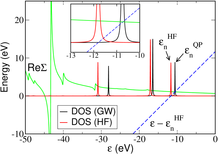
Figure 3: (Color online) Density of states for the NH₃ molecule calculated in HF and GW, respectively. Arrows mark the level corresponding to the HOMO in the two calculations. The intersection between the line $y=\varepsilon-\varepsilon_{n}^{\text{HF}}$ and the real part of $\langle\psi^{0}_{\text{HOMO}}|\Sigma_{\text{corr}}(\varepsilon)|\psi_{\text{HOMO}}^{0}\rangle$ (green curve) determines the position of the GW level.

III.1 Linearized quasiparticle equation

In the conventional GW method the full Green function of Eq. (2) is not calculated. Rather one obtains the quasiparticle energies from the quasiparticle equation

$$\varepsilon_{n}^{\text{QP}}=\varepsilon_{n}^{0}+Z_{n}\langle\psi_{n}^{0}|\Sigma_{\text{GW}}(\varepsilon_{n}^{0})-v_{\text{xc}}|\psi_{n}^{0}\rangle.$$ (14)

where $\psi_{n}^{0}$ and $\varepsilon_{n}^{0}$ are eigenstates and eigenvalues of an approximate single-particle Hamiltonian (often the LDA Hamiltonian), and

$$Z_{n}=\Big{[}1-\frac{\partial\langle\psi_{n}^{\text{DFT}}|\Sigma_{\text{GW}}(\varepsilon)|\psi_{n}^{0}\rangle}{\partial\varepsilon}\Big{|}_{\varepsilon_{n}^{0}}\Big{]}^{-1}.$$ (15)

Moreover the GW self-energy is evaluated non-selfconsistently from the single-particle Green function, i.e. $\Sigma_{\text{GW}}=iG_{0}W[G_{0}]$, with $G_{0}(z)=(z-H_{0})^{-1}$.

The quasiparticle equation (14) relies on the assumption that off-diagonal matrix elements, $\langle\psi_{n}^{0}|\Sigma_{\text{GW}}(\varepsilon_{n}^{0})-v_{\text{xc}}|\psi_{m}^{0}\rangle$, can be neglected, and that the frequency dependence of $\Sigma_{\text{GW}}$ can be approximated by its first order Taylor expansion in a sufficiently large neighborhood of $\varepsilon_{n}^{0}$. We have found that these two assumptions are indeed fullfilled for the molecular systems studied here. More precisely, for the GW and G₀W₀(HF) self-energies, the QP energies obtained from Eq. (14) are always very close to the peaks in the density of states Eq. (9). We emphasize that this result could well be related to the rather large level spacing of small molecules, and may not hold for extended systems. An example is presented in Fig. 3 which shows the full HF and GW density of states for NH₃ together with the real part of $\langle\psi^{0}_{\text{HOMO}}|\Sigma_{\text{corr}}(\varepsilon)|\psi_{\text{HOMO}}^{0}\rangle$. As explained in the following section this is not quite the case for the G₀W₀(PBE) calculations.

III.2 $G_{0}$-dependence

As stated in the previous section the GW and G₀W₀(HF) energies can be obtained either from the full spectral function or from the QP equation. In this case, returning to Table 1, we see that G₀W₀(HF) yields systematically larger IPs than GW. This is easy to understand since $G_{\text{HF}}$ describes a larger HOMO-LUMO gap than $G_{\text{GW}}$, and therefore produces less screening. When the PBE rather than the HF Green function is used to evaluate the GW self-energy, we find that the spectral function obtained from Eq. (2) does not resemble a simple discrete spectrum. In fact the peaks are significantly broadened by the imaginary part of $\Sigma_{\text{GW}}$ and it becomes difficult to assign precise values to the QP energies. Apart from the spectral broadening, the molecular gap is significantly reduced with respect to its value in the GW and G₀W₀(HF) calculations. Both of these effects are due to the very small HOMO-LUMO gap described by $G_{\text{PBE}}$ which leads to severe overscreening and QP life-time reductions. A similar effect was observed by Ku and Eguiluz in their comparison of GW and G₀W₀(LDA) for Si and Ge crystalsku .

The problems encountered when attempting to solve the Dyson equation (2) using the G₀W₀(PBE) self-energy occur due to the large mismatch between $\varepsilon_{n}^{\text{PBE}}$ and $\varepsilon_{n}^{\text{QP}}$. On the other hand, in the QP equation, the GW self-energy is evaluated at $\varepsilon_{n}^{0}$ rather than $\varepsilon_{n}^{\text{QP}}$. As a consequence the unphysical broadening and overscreening is avoided and a well defined QP energy can be obtained (last column in Table 1).

To summarize, $G_{0}$ can have a very large effect on the QP spectrum when the latter is obtained via the Dyson equation (2). In particular, the use of a $G_{0}$ with a too narrow energy gap (as e.g. the $G_{\text{PBE}}$) can lead to unphysical overscreening and spectral broadening. When the QP levels are obtained from the QP equation, the $G_{0}$-dependence is less pronounced because $\Sigma_{\text{GW}}[G_{0}]$ is evaluated at $\varepsilon_{n}^{0}$ which is consistent with $G_{0}$.

The self-consistent GW spectrum is independent of the choice of $G_{0}$, but the number of iterations required to reach self-consistency is less when based on $G_{\text{HF}}$.

III.3 Basis set convergence

In Figs. 4 and 5 we show the energy of the three highest occupied molecular orbitals of H₂O and CO obtained from selfconsistent GW using various sizes of the augmented Wannier basis. Clearly, the polarization functions have relatively little influence on the QP energies while the first set of additional zeta functions reduce the QP energies by up to 0.5 eV. The differences between DZP and TZDP are less than 0.15 eV for all the levels which justifies the use of DZP basis.

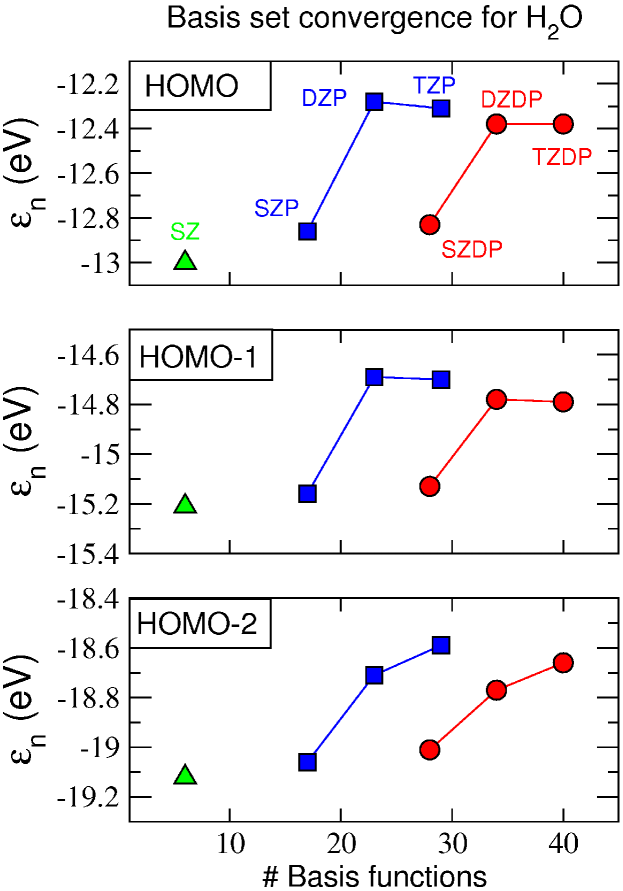
Figure 4: (Color online) Convergence of the three highest occupied levels of H₂O obtained from GW calculations with different sizes of the augmented Wannier function basis. SZ denotes the Wannier function basis, while e.g. DZDP denotes the Wannier basis augmented by one extra radial function per valence state and two sets of polarization functions.

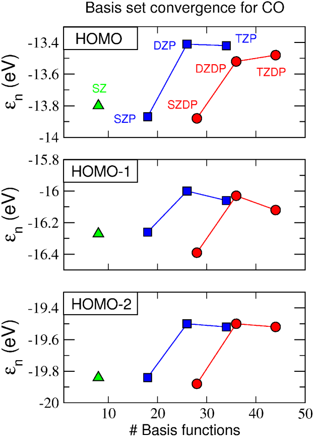
Figure 5: (Color online) Same as Fig. 4 but for CO.

We have also compared the eigenvalues obtained from selfconsistent HF calculations using the DZP augmented Wannier basis to accurate HF calculations performed with the real-space code GPAWGPAW . Here we obtain a MAE of 0.09 eV for the energy of the HOMO level of the 33 molecules.

IV Conclusions

As the range of systems to which the GW method is being applied continues to expand it becomes important to establish its performance for other systems than the solids. In this work we have discussed benchmark GW calculations for molecular systems.

The GW calculations were performed using a novel scheme based on the PAW method and a basis set consisting of Wannier functions augmented by numerical atomic orbitals. We found that a basis corresponding to double-zeta with polarization functions was sufficient to obtain GW energies converged to within  0.1 eV (compared to triple-zeta with double polarization functions). The GW self-energy was calculated on the real frequency axis including its full frequency dependence and off-diagonal elements. We thereby avoid all of the commonly used approximations, such as the the plasmon pole approximation, the linearized quasiparticle equation and analytical continuations from imaginary to real frequencies, and thus obtain a direct and unbiased assessment of the GW approximation itself. We found that the inclusion of valence-core exchange interactions, as facilitated by the PAW method, is important and affect the HF/GW HOMO levels by -1.2 eV on average.

The position of the HOMO for a series of 33 molecules was calculated using fully selfconsistent GW, single-shot G₀W₀, Hartree-Fock, DFT-PBE0, and DFT-PBE. Both PBE and PBE0 eigenvalues grossly overestimate the HOMO energy with a mean absolute error (MAE) with respect to the experimental ionization potentials (IP) of 4.4 and 2.5 eV, respectively. Hartree-Fock underestimates the HOMO energy but improves the agreement with experiments yielding a MAE of 0.8 eV. GW and G₀W₀ overcorrects the Hartree-Fock levels slightly leading to a small overestimation of the HOMO energy with a MAE relative to experiments of 0.4-0.5 eV. This shows that although screening is a weak effect in molecular systems its inclusion at the GW level improves the electron removal energies by 30-50% relative to the unscreened Hartree-Fock. The best IPs were obtained from one-shot G₀W₀ calculations starting from the HF Green’s function where the overscreening is least severe. Very similar conclusions were reached by comparing GW, G₀W₀ and HF to exact diagonalization for conjugated molecules described by the semi-empirical PPP model.paperI

V Acknowledgments

We thank Mikkel Strange for useful discussions and assistance with the projected Wannier functions. We acknowledge support from the Danish Center for Scientific Computing and The Lundbeck Foundation’s Center for Atomic-scale Materials Design (CAMD).

Appendix A The GW self-energy

Let $U$ denote the rotation matrix that diagonalizes the pair orbital overlap $S_{ij,kl}=\langle n_{ij}|n_{kl}\rangle$, i.e. $U^{\dagger}SU=\sigma I$. The columns of $U$ are truncated to those which have corresponding eigenvalues $\sigma_{q}<10^{-5}a_{0}^{-3}$. We then only calculate the reduced number of Coulomb elements

$$V_{qq^{\prime}}=\langle n_{q}|\frac{1}{|\bm{r}-\bm{r}^{\prime}|}|n_{q^{\prime}}\rangle,$$ (16)

where $n_{q}(\bm{r})$ are the optimized pair orbitals

$$n_{q}(\bm{r})=\sum_{ij}n_{ij}(\bm{r})U_{ij,q}/\sqrt{\sigma_{q}},$$ (17)

which are mutually orthonormal, i.e. $\langle n_{q}|n_{q^{\prime}}\rangle=\delta_{qq^{\prime}}$.

Determining the GW self-energy proceeds by calculating first the full polarization matrix in the time domain

$$P^{<}_{ij,kl}(t) =2iG^{<}_{ik}(t)G^{>*}_{jl}(t),$$ (18)

$$P^{>}_{ij,kl}(t) =P^{<*}_{ji,lk}(t).$$ (19)

The factor 2 appears for spin-paired systems from summing over spin indices. This is then downfolded to the reduced representation

$$P^{\lessgtr}_{qq^{\prime}}=\sum_{ij,kl}\sqrt{\sigma_{q}}U^{*}_{ij,q}P^{\lessgtr}_{ij,kl}U_{kl,q^{\prime}}\sqrt{\sigma_{q^{\prime}}}.$$ (20)

The screened interaction can be determined from the lesser and greater polarization matrices, and the static interaction $V_{qq^{\prime}}$, via the relations

$$P^{r}(t) =\theta(t)\left(P^{>}(t)-P^{<}(t)\right),$$ (21)

$$W^{r}(\varepsilon) =[I-VP^{r}(\varepsilon)]^{-1}V,$$ (22)

$$W^{>}(\varepsilon) =W^{r}(\varepsilon)P^{>}(\varepsilon)W^{r\dagger}(\varepsilon),$$ (23)

$$W^{<}(\varepsilon) =W^{>}(\varepsilon)-W^{r}(\varepsilon)+W^{r\dagger}(\varepsilon),$$ (24)

where all quantities are matrices in the optimized pair orbital basis and matrix multiplication is implied. We obtain the screened interaction in the original orbital basis from

$$W^{\lessgtr}_{ij,kl}(t)\approx\sum_{qq^{\prime}}U_{ij,q}\sqrt{\sigma_{q}}W^{\lessgtr}_{qq^{\prime}}(t)\sqrt{\sigma_{q^{\prime}}}U_{kl,q^{\prime}}^{*},$$ (25)

which is an approximation due to the truncation of the columns of U. Finally the GW self-energy can be determined by

$$\Sigma^{\lessgtr}_{\text{GW,}ij}(t) =i\sum_{kl}G^{\lessgtr}_{kl}(t)W^{\lessgtr}_{ik,jl}(t)$$ (26)

$$\Sigma^{r}_{\text{GW}}(t) =\theta(t)\left(\Sigma^{>}_{\text{GW}}(t)-\Sigma^{<}_{\text{GW}}(t)\right)+\delta(t)\Sigma_{x}.$$ (27)

The exchange and Hartree potentials are given by

$$\Sigma_{x,ij} =i\sum_{kl}V_{ik,jl}G^{<}_{kl}(t=0)$$ (28)

$$\Sigma_{\text{H},ij} =-2i\sum_{kl}V_{ij,kl}G^{<}_{kl}(t=0)$$ (29)

The Green functions are given by

$$G^{r}(\varepsilon)= [(\varepsilon+i\eta)S-H_{\text{KS}}+v_{\text{xc}}-\Delta v_{\text{H}}-\Sigma_{\text{GW}}^{r}(\varepsilon)]^{-1}$$ (30)

$$G^{<}(\varepsilon)= -f_{\text{FD}}(\varepsilon-\mu)[G^{r}(\varepsilon)-G^{r}(\varepsilon)^{\dagger}]$$ (31)

$$G^{>}(\varepsilon)= (1-f_{\text{FD}}(\varepsilon-\mu))[G^{r}(\varepsilon)-G^{r}(\varepsilon)^{\dagger}]$$ (32)

where $f_{\text{FD}}(\varepsilon-\mu)$ is the Fermi-Dirac function and $\Delta v_{\text{H}}=\Sigma_{\text{H}}[G]-\Sigma_{\text{H}}[G_{\text{DFT}}]$ is the difference between the GW Hartree potential and the DFT Hartree potential. For self-consistent calculations, equation (18)-(32) are iterated untill convergence in $G$.

References

- (1) P. Hohenberg and W. Kohn Phys. Rev. 136, B864 (1964).
- (2) W. Kohn and L. J. Sham Phys. Rev. 140, A1133 (1965).
- (3) M. S. Hybertsen and S. G. Louie, Phys. Rev. B 34, 5390 (1986).
- (4) J. P. Perdew and A. Zunger, Phys. Rev. B 23, 5048 (1981).
- (5) J. Paier, M. Marsman, K. Hummer, G. Kresse, I. C. Gerber, and J. G. Angyan, J. Chem. Phys. 124, 154709 (2006)
- (6) J. Heyd, J. E. Peralta, G. E. Scuseria, and R. L. Martin, J. Chem. Phys. 123, 174101 (2005).
- (7) C. Adamo and V. Barone, J. Chem. Phys. 110, 6158 (1999)
- (8) A. D. Becke, J. Chem. Phys. 98, 5648 (1993)
- (9) C. Lee, W. Yang and R. G. Parr, Phys. Rev. B 37, 785 (1988)
- (10) J. Heyd, G. E. Scuseria, and M. Ernzerhof, J. Chem. Phys. 118, 8207 (2003)
- (11) According to Janak’s theoremjarnak , for finite systems the position of the HOMO in exact Kohn-Sham theory should coincide with the ionization potential. However, for practical exchange-correlation functionals this is far from being the caseperdew_zunger ; pemmaraju07 .
- (12) J. F. Jarnak, Phys. Rev. B 18, 7165 (1978).
- (13) C. D. Pemmaraju, T. Archer, D. Sanchez-Portal, and S. Sanvito, Phys. Rev. B 75, 045101 (2007)
- (14) J. Q. Sun and R. J. Bartlett, J. Chem. Phys. 104, 8553 (1996)
- (15) L. Dagens and F. Perrot, Phys. Rev. B 5, 641 (1972)
- (16) Solid State Physics, G. Grosso and G. P. Parravicini, Cambridge University Press, Cambridge 2000
- (17) L. Hedin, Phys. Rev. 139, A796 (1965)
- (18) F. Aryasetiawan and O. Gunnarson, Rep. Prog. Phys. 61, 237 (1998)
- (19) W. G. Aulbur, L. Jonsson, and J. Wilkins, in Solid State Physics, edited by H. Ehrenreich and F. Saepen (Academic Press, New York 2000), Vol. 54, 1.
- (20) G. Onida, L. Reining, and A. Rubio, Rev. Mod. Phys. 74, 601 (2002)
- (21) J. C. Grossman, M. Rohlfing, L. Mitas, S. G. Louie, and M. L. Cohen, Phys. Rev. Lett. 86, 472 (2001).
- (22) P. H. Hahn, W. G. Schmidt, and F. Bechstedt Phys. Rev. B 72, 245425 (2005)
- (23) T. Niehaus, M. Rohlfing, F. D. Sala, A. Di Carlo, and T. Frauenhaim, Phys. Rev. A 71, 022508 (2005)
- (24) A. Stan, N. E. Dahlen, and R. van Leeuwen, Europhys. Lett. 76, 298 (2006)
- (25) C. D. Spataru, S. Ismail-Beigi, X. L. Benedict, and S. G. Louie, Phys. Rev. Lett. 92, 077402 (2004)
- (26) P. E. Trevisanutto, C. Giorgetti, L. Reining, M. Ladisa, and V. Olevano, Phys. Rev. Lett. 101, 226405 (2008)
- (27) M. L. Tiago and J. R. Chelikowsky, Phys. Rev. B 73, 205334 (2006)
- (28) J. B. Neaton, M. S. Hybertsen, and S. G. Louie Phys. Rev. Lett. 97, 216405 (2006)
- (29) K. S. Thygesen and A. Rubio, Phys. Rev. Lett. 102, 046802 (2009)
- (30) C. Freysoldt and P. Rinke and M. Scheffler, Phys. Rev. Lett. 103, 056803 (2009)
- (31) J. M. Garcia-Lastra, C. Rostgaard, A. Rubio, and K. S. Thygesen Phys. Rev. B 80, 245427 (2009)
- (32) K. S. Thygesen and A. Rubio, J. Chem. Phys. 126, 091101 (2007).
- (33) K. S. Thygesen, Phys. Rev. Lett. 100, 166804 (2008)
- (34) P. Myöhanen and A. Stan and G. Stefanucci and R. van Leeuwen, Euro. Phys. Lett. 84, 67001 (2008)
- (35) C. D. Spataru and M. S. Hybertsen and S. G. Louie and A. J. Millis, Phys. Rev. B 79, 155110 (2009)
- (36) M. P. von Friesen and C. Verdozzi and C.-O. Almbladh, Phys. Rev. Lett. 103, 176404 (2009)
- (37) K. Kaasbjerg and K. S. Thygesen (submitted)
- (38) B. Holm and U. von Barth Phys. Rev. B 57, 2108 (1998)
- (39) M. Usuda, N. Hamada, T. Kotani, and M. van Schiflgaarde, Phys. Rev. B 66, 125101 (2002)
- (40) W. Ku and A. G. Eguiluz, Phys. Rev. Lett. 89, 126401 (2002)
- (41) M. van Schiflgaarde, T. Kotani, and S. V. Faleev, Phys. Rev. B 74, 245125 (2006)
- (42) M. Shishkin and G. Kresse, Phys. Rev. B 74, 035101 (2006)
- (43) P. Rinke, A. Qteish, J. Neugebauer, C. Freysoldt, and M. Scheffler New J. Phys. 7 126 (2005)
- (44) X. Qian, J. Li, L. Qi, C.-Z. Wang, T.-L. Chan, Y.-X. Yao, K.-M. Ho, and S. Yip, Phys. Rev. B 78, 245112 (2008)
- (45) J. J. Mortensen, L. B. Hansen, K. W. Jacobsen, Phys. Rev. B 71, 035109 (2005)
- (46) A. H. Larsen, M. Vanin, J. J. Mortensen, K. S. Thygesen, and K. W. Jacobsen Phys. Rev. B 80, 195112 (2009)
- (47) K. S. Thygesen and A. Rubio, Phys. Rev. B 77, 115333 (2008).
- (48) K. S. Thygesen, Phys. Rev. B 73, 035309 (2006)
- (49) H. Haug and A. -P. Jauho, Quantum Kinetics in Transport and Optics of Semiconductors, Springer (1998)
- (50) R.van Leeuwen, N.E.Dahlen, G.Stefanucci, C.-O.Almbladh, and U.von Barth, Lectures Notes in Physics vol. 706 (Springer)
- (51) A. Stan, N. E. Dahlen, and R. van Leeuwen, J Chem. Phys. 130, 114105 (2009)
- (52) F. Aryasetiawan and O. Gunnarsson, Phys. Rev. B 49, 16214 (1994)
- (53) M. Walter, H. Häkkinen, L. Lehtovaara, M. Puska, J. Enkovaara, C. Rostgaard, and J. J. Mortensen, J Chem. Phys. 128, 244101 (2009)
- (54) P. E. Blöchl, Phys. Rev. B 50, 17953 (1994)
- (55) E. Engel, Phys. Rev. B 80, 161205(R) (2009)
- (56) L. A. Curtiss, K. Raghavachari, P. Redfern, and J. A. Pople, J. Chem. Phys. 106, 1063 (1997).
- (57) J. P. Perdew, K. Burke, M. Ernzerhof, Phys. Rev. Lett. 77, 3865 (1996)
- (58) M. van Schilfgaarde, T. Kotani, and S. Faleev, Phys. Rev. Lett. 96, 226402 (2006)
- (59) NIST Computational Chemistry Comparison and Benchmark Database, NIST Standard Reference Database Number 101 Release 14, Sept 2006, Editor: Russell D. Johnson III http://srdata.nist.gov/cccbdb