Chapter 3 Theory and Simulation of Multiphase Polymer Systems

Friederike Schmid

Institute of Physics, Johannes-Gutenberg Universität Mainz, Germany

I Introduction

The theory of multiphase polymer systems has a venerable tradition. The ’classical’ theory of polymer demixing, the Flory-Huggins theory, was developed already in the forties of the last century [1, 2]. It is still the starting point for most current approaches – be they improved theories for polymer (im)miscibility that take into account the microscopic structure of blends more accurately, or sophisticated field theories that allow to study inhomogeneous multicomponent systems of polymers with arbitrary architectures in arbitrary geometries. In contrast, simulations of multiphase polymer systems are relatively young. They are still limited by the fact that one must simulate a large number of large molecules in order to obtain meaningful results. Both powerful computers and smart modeling and simulation approaches are necessary to overcome this problem.

In the limited space of this chapter, I can only give a taste of the state-of-the-art in both areas, theory and simulation. Since the theory has reached a fairly mature stage by now, many aspects of it are covered in textbooks on polymer physics [3, 4, 5, 6, 7, 8, 9, 8]. The information on the state-of-the art of simulations is much more scattered. This is why I have put some effort into putting together a representative list of references in this area – which is of course still far from complete.

The chapter is organized as follows. In Section II, I briefly introduce some basic concepts of polymer theory. The purpose of this part is to make the chapter accessible to readers who are not very familiar with polymer physics; it can safely be skipped by the others. Section III is devoted to the theory of multiphase polymer systems. I recapitulate the Flory-Huggins theory and introduce in particular the concept of the Flory interaction parameter (the $\chi$ parameter), which is a central ingredient in most theoretical descriptions of multicomponent polymer systems. Then I focus on one of the most successful mean-field theories for inhomogeneous (co)polymer blends, the self-consistent field theory. I sketch the main idea, discuss various aspects of the theory and finally derive popular analytical approximations for weakly and strongly segregated blends (the random phase approximation and the strong-segregation theory).

In Section IV, I turn to discussing simulations of multiphase polymer systems. A central concept in this research area is ’multiscale modeling’: Polymers cannot be treated at all levels of detail simultaneously, hence coarse-grained models are used in order to study different aspects of the materials in different simulations. This allows one to push the simulation limits to larger length and time scales. I describe some of the most popular coarse-grained structural and dynamical models and give an overview over the state-of-the-art of simulations of polymer blends and copolymer melts.

II Basic Concepts of Polymer Theory

For the sake of readers who are not familiar with polymer theory, I begin with recapitulating very briefly some basic concepts.

Polymers are macromolecules containing up to hundreds of thousands of atoms. At first sight, one would not expect such molecules to be easily amenable to theoretical modeling; however, it turns out that the large size of the molecules and their highly repetitive structure in fact simplifies things considerably. Since polymer molecules interact with many others, details of local interactions average out and polymers can often be characterized by a few effective quantities, such as their topology, the local stiffness along the backbone, the bulkiness, the compatibility/incompatibility of the building blocks etc. Already decades ago, pioneers like Flory [3], Edwards [5], de Gennes[4] have established theoretical polymer science as a highly successful field of research, which brings together scientists from theoretical chemistry, statistical physics, materials science, and even the biosciences, has created a wealth of new beautiful theoretical concepts, and has not lost any of its fascination for theorists up to date.

II.1 Fundamental Properties of Polymer Molecules

The characterizing property of polymers is their highly modular structure. They are composed of a large number of small building blocks (monomers), which are often all alike, but may also be combined to arbitrary sequences (in the case copolymers and biopolymers). The monomers are arranged in chains, which are usually flexible on the nanometer length scale, i.e., they can form kinks at little energetic expense, they curve around and may assume a large number of conformations at room temperature. The properties of such flexible polymers are largely determined by the entropy of the chain conformations. For example, the number of available conformations is reduced if molecules are stretched, which leads to a purely entropic restoring spring force[10] (rubber elasticity). Exposed to stress, polymeric systems respond by molecular rearrangements, which takes time and results in time-dependent strain (viscoelasticity).

The fundamental processes that govern the behavior of polymeric materials do not depend on the chemical details of the monomer structure. For qualitative purposes, polymer molecules can be characterized by a few properties such as

• The architecture of the molecules (linear chains, rings, stars, etc.)

• Physical properties (local chain stiffness, chain size, monomer volume)

• Physicochemical properties (monomer sequence, compatibility, charges)

• Special properties (e.g., a propensity to develop crystalline or liquid crystalline order).

II.2 Coarse-Graining, Part I

The notion of ’coarse-graining’ has lately become a buzzword in materials science, but the underlying concept is actually quite old in polymer science. The need for coarse-graining results from the fact that polymeric materials exhibit structure on very different length scales, ranging from Angstrom (the monomeric scale) to hundreds of nanometers (typical molecule extensions) or micrometers (supramolecular aggregates). It is not possible to treat all of them within one common theoretical framework. Therefore, different theoretical descriptions have been developed that deal with phenomena on different length and time scales. On the microscale, chemical details are taken into account and the polymers are treated at an atomistic level. This is the realm of theoretical chemistry. On the mesoscale, simplified molecule models come into play (string models, lattice models, bead-spring models, see below), whose behavior can be understood with concepts from statistical physics. Finally, on the macroscale, polymeric materials are described by continuous fields (composition, strain, stress etc.) with certain mechanical properties, and their behavior can be calculated with methods borrowed from the engineers.

In the following, I shall mainly focus on the mesoscale level, where polymers are described by extended molecules made of simplified ”monomeric” units, each representing several real monomers. Even within that level, one still has some freedom regarding the choice of the coarse-grained units. This is illustrated in Fig. 3.1, where different coarse-grained representations of a polymer are superimposed onto each other. Polymers have remarkable universality properties, which allow one to link different coarse-grained representations in a rather well-defined manner, as long as the length scales under consideration are much larger than the (chemical) monomer length scale. For example, starting from one (atomistic or coarse-grained) model, we can construct a coarse-grained model by combining $m$ ”old” units to one ”new” unit. If $m$ is sufficiently large, the average squared distance $\langle d^{2}\rangle$ between two adjacent new units will depend on $m$ according to a characteristic power law

$$\langle d^{2}\rangle\sim m^{2\nu},$$ (3.1)

where the exponent $\nu$ depends on the environment of a polymer, but not on chemical details [4, 5]. In a dense polymer melt, one has $\nu=1/2$ (see below). Similar scaling laws can be established for other chain parameters.

Figure 3.1: Mesoscopic coarse-grained representations of a polymer molecule. Light pearl necklace in the background: Bead chain with bonds of fixed length. Solid and dashed lines, chain of coarse-grained units linked by bonds of variable length.

II.3 Ideal Chains

In mesoscopic polymer theories, one often uses as a starting point a virtual polymer chain where monomers that are well separated along the polymer backbone do not interact with each other, even if their spatial distance is small. Such polymers are called ’ideal chains’. Even though they are mere theoretical constructions, they provide a good approximative description of polymers in melts and in certain solvents (’Theta’-solvents, see below).

II.3.1 A Paradigm of Polymer Theory: The Gaussian Chain

Let us now consider a flexible ideal chain with $N$ monomers, which we coarse-grain several times as sketched in Fig. 3.1, until one coarse-grained monomer unites $m$ ’real’ monomers. For large $m$, the resulting chain is a random walk in space consisting of uncorrelated random steps ${\bf d}_{i}$ of varying length. According to the central limit theorem of probability theory [11], the steps are approximately Gaussian distributed, ${\cal P}({\bf d})\sim\exp(-d^{2}/2m\sigma^{2})$, where $\sigma$ does not depend on $m$. The same random walk statistics can be reproduced by a Boltzmann distribution with an effective coarse-grained Hamiltonian

$${\cal H}_{m}=\frac{1}{2}\>\frac{k_{{}_{B}}\!T}{m\sigma^{2}}\sum_{i=1}^{N/m}{\bf d}_{i}^{2}.$$ (3.2)

The Hamiltonian ${\cal H}_{m}$ describes the energy of a chain of springs with spring constant $k_{{}_{B}}\!Tm/\sigma^{2}$. The coarse-graining procedure has thus eliminated the information on chemical details (they are now incorporated in the single parameter $\sigma$), and instead unearthed the entropically induced elastic behavior of the chain which lies at the heart of rubber elasticity. Eq. (3.2) is also an example for universal behavior in a polymer system (see section II.2): The coarse-grained chain is self-similar. Every choice of $m$ produces an equivalent model, provided the spring constant is rescaled accordingly. The distance between two coarse-grained units exhibits a scaling law of the form (3.1) as a function of $m$, $\langle d^{2}\rangle=3\sigma^{2}m^{2\nu}$ with $\nu=1/2$.

Based on these considerations, it seems natural to define a ’generic’ ideal chain model based on Eq. (3.2) with $m=1$,

$$\frac{{\cal H}_{G}[{\bf r}_{i}]}{k_{{}_{B}}\!T}=\frac{1}{2\sigma^{2}}\>\sum_{i=1}^{N-1}({\bf r}_{i+1}-{\bf r}_{i})^{2},$$ (3.3)

the so-called ’discrete Gaussian chain’ model. For theoretical purposes, it is often convenient to take the continuum limit: The index $i$ in Eq. (3.2), which counts the monomers along the chain backbone, is replaced by a continuous variable $s$, the chain is parametrized by a continuous path ${\bf R}(s)$, and the steps ${\bf d}$ correspond to the local derivatives ${\rm d}{\bf R}/{\rm d}s$ of this path. The effective Hamiltonian then reads

$$\frac{{\cal H}_{G}[{\bf R}]}{k_{{}_{B}}\!T}=\frac{3}{2b^{2}}\int_{0}^{N}{\rm d}s\>\big{(}\frac{{\rm d}{\bf R}}{{\rm d}s}\big{)}^{2}.$$ (3.4)

This defines the continuous Gaussian chain. The only material parameters in Eq. (3.4) are the chain length $N$ and the ’statistical segment length’ or ’Kuhn length’ $b$. Even those two are not independent, since they both depend on the definition of the monomer unit. An equivalent chain model can be obtained by rescaling $N\to N/\lambda$ and $b^{2}\to b^{2}\lambda$. Hence the only true independent parameter is the extension of the chain, which can be characterized by the squared gyration radius

$$R_{g}^{2}=\frac{1}{N}\int_{0}^{N}{\rm d}s\>({\bf R}(s)-\overline{{\bf R}})^{2}=b^{2}N/6,$$ (3.5)

where $\overline{{\bf R}}=1/N\int{\rm d}s\>{\bf R}(s)$ is the center of mass of the chain. The quantity $R_{g}$ sets the (only) characteristic length scale of the Gaussian chain, and all length-dependent quantities scale with $R_{g}$. For example, the structure factor is given by

$$S({\bf k})=\frac{1}{N}\langle\left|\int_{0}^{N}{\rm d}s\>e^{i{\bf k\>R}(s)}\right|^{2}\rangle=Ng_{{}_{D}}\!(k^{2}R_{g}^{2}),$$ (3.6)

with the Debye function

$$g_{{}_{D}}\!(x)=\frac{2}{x^{2}}(e^{-x}-1+x).$$ (3.7)

The Gaussian chain is not only a prototype model for ideal chains, it also provides a general framework for mesoscopic theories of polymer systems. The Hamiltonian ${\cal H_{G}}$ (Eq. (3.4)) is then supplemented by additional terms that account for interactions, external fields, constraints (e.g., chemical crosslinks) etc. In this more general context, the Hamiltonian (3.4) is often referred to as ’Edwards Hamiltonian’.

Finally in this section, let us note that from a mathematical point of view, the probability distribution of chain conformations defined by Eq. (3.4) is a Wiener measure [11, 12]. The continuum limit leading to Eq. (3.4) is far from trivial, but well-defined. I shall not dwell further into this matter.

II.3.2 Other Chain Models

The Gaussian chain model is a common starting point for analytical theories of long flexible polymers on sufficiently large length scales. On smaller length scales, or for stiffer polymers, or for computer simulation purposes, other types of coarse-grained models have proven useful. I briefly summarize some popular examples.

The wormlike chain model is a continuous model designed to describe stiff polymers. They are represented by smooth paths ${\bf R}(s)$ with fixed contour length $N$, where the parameter $s$ runs over the arc length of the curve, i.e., the derivative vector ${\bf u}={\rm d}{\bf R}/{\rm d}s$ has length unity, $|{\bf u}|\equiv 1$. The paths have a bending stiffness $\eta$, such that they are distributed according to the effective Hamiltonian

$$\frac{{\cal H}_{WLC}[{\bf R}]}{k_{{}_{B}}\!T}=\frac{\eta}{2}\int_{0}^{N}{\rm d}s\>\big{(}\frac{{\rm d}^{2}{\bf R}}{{\rm d}s^{2}}\big{)}^{2}.$$ (3.8)

The wormlike chain model is particularly useful if local orientational degrees of freedom are important.

The freely jointed chain is a discrete chain model where the chain is composed of $N$ links of fixed length. It is often used to study general properties of ideal chains.

The spring-bead chain is a chain of beads connected with springs. It has some resemblance with the discrete Gaussian chain model, except that the springs have a finite equilibrium length. Spring-bead models are popular in computer simulations.

In lattice models, the monomer positions are confined to the sites of a lattice. This simplifies both theoretical considerations and computer simulations.

II.4 Interacting Chains

The statistical properties of chains change fundamentally if monomers interact with each other. Such interactions are readily introduced in the coarse-grained models presented above. In the discrete models, one simply adds explicit interactions between monomers. In the continuous path models, one supplements the energy contribution for individual ideal chains, Eq. (3.4) or (3.8), by an interaction term, such as

$${\cal H}_{I}[\hat{\rho}]=\frac{v}{2}\int{\rm d}{\bf r}\>\hat{\rho}^{2}+\frac{w}{6}\int{\rm d}{\bf r}\>\hat{\rho}^{3}+\cdots$$ (3.9)

(for weak interactions), where the ’monomer density’ $\hat{\rho}(\bf r)$ is defined as

$$\hat{\rho}({\bf r})=\sum_{\alpha}\int_{0}^{N}{\rm d}s\>\delta({\bf r}-{\bf R}_{\alpha}(s))$$ (3.10)

and the sum $\alpha$ runs over the polymers ${\bf R}_{\alpha}(s)$ in the system. Eq. (3.9) corresponds to a virial expansion of the local interaction energy in powers of the density. In many cases, only the quadratic term ($v$) needs to be taken into account (’two-parameter Edwards model’). The Ansatz (3.9) is suitable for dilute polymer systems – dense systems are discussed below (Sec. II.4.2). The generalization to multiphase systems where monomers may have different type A,B,$\cdots$ is straightforward. One simply operates with different densities $\hat{\rho}_{A},\hat{\rho}_{B},\cdots$ and interaction parameters $v_{AA},v_{AB},\cdots$.

Interactions complicate the theoretical treatment considerably and in general, exact analytical solutions are no longer available. The properties of interacting polymer systems have been explored theoretically within mean-field approximations, renormalization-group calculations, scaling arguments, and computer simulations. To set the stage for the discussion of multiphase systems in sections III and IV, I will now briefly sketch the most important scenarios for monophase polymer systems.

II.4.1 Polymers in Solution and Blobs

We first consider single, isolated polymer chains in solution. Their properties depend on the quality of the solvent, which is incorporated in the second virial parameter $v$ in Eq. (3.9) (the three-body parameter $w$ is typically positive[13]). In good solvent ($v>0$), monomers effectively repel each other, and the chain swells. Extensive theoretical work [4] has shown that the scaling behavior (Eq. (3.1)) remains valid, but the exponent $\nu$ increases from $\nu=1/2$ for ideal chains to $\nu\approx 3/(d+2)$, where $d$ is the spatial dimension (more precisely, $\nu=0.588$ in three dimensions). This is the famous ’Flory exponent’, which characterizes the scaling behavior of so-called ’self-avoiding chains’. Accordingly, the gyration radius of the chain scales with the chain length like

$$R_{g}^{2}\sim N^{2\nu}.$$ (3.11)

In poor solvent ($v<0$), monomers effectively attract each other and the chain collapses. At the transition between the two regimes, the ’Theta point’ ($v_{\theta}\approx 0$), the scaling behavior basically corresponds to that of ideal chains ($\nu=1/2$), except for subtle corrections due to the three-body $w$-term [4].

Eq. (3.11) describes the behavior of single, unperturbed chains. Even in good solvent, the self-avoiding scaling is often disturbed. For example, the chains cannot swell freely if they are confined, or if they are subject to external forces. Another important factor is the concentration of chains in the solution: If many chains overlap, the intrachain interactions are screened on large length scales. Loosely speaking, monomers cannot distinguish between interactions with monomers from the same chain and from other chains. As a result, chains no longer swell and ideal chain behavior is recovered. This mechanism applies in three or more spatial dimensions. Two dimensional chains segregate [4, 14, 15].

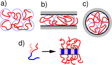
Figure 3.2: Illustration of the blob model in different situations: a) concentrated polymer solution b) Polymer confined in a slit c) chain confined in a spherical cavity d) structure formation in solutions of miktoarm star copolymers (after Ref. 16). See text for explanation.

All of these situations can be analyzed within one single ingenious framework, the ’blob’ picture introduced Daoud et al. in 1975 [17]. It is based on the assumption that there exists a crossover length scale $\xi$ below which the chain is unperturbed. Blobs are volume elements of size $\xi$ within which the polymers behave like self-avoiding chains. On larger scales, the polymer behaves like an ideal chain consisting of a string of blobs. Every blob contains $m\sim\xi^{1/\nu}$ monomers and carries a free energy of the order $k_{{}_{B}}\!T$. These simple rules are the whole essence of the blob model. I shall illustrate their use by applying them to a number of prototype situations depicted in Fig. 3.2.

Concentrated polymer solution (Fig. 3.2 a). For polymer concentrations $\phi$, we calculate the crossover length scale $\xi$ from self-avoiding to ideal behavior. Since $\xi$ is the blob size, we can simply equate $\phi=m/\xi^{3}$, i.e., $\xi\sim\phi^{-\nu/(3\nu-1)}$.

Polymer confined in a slit (Fig. 3.2 b). We consider the free energy penalty $F$ on the confinement. Here, the blob size is set by the width $R$ of the slit. Each blob contains $m\sim R^{1/\nu}$ monomers, hence the total free energy scales like $F\sim N/m\sim NR^{-1/\nu}$.

Polymer confined in a cavity (Fig. 3.2 c) The result b) also holds for chains confined in a tube. In closed cavities, however, the situation is different due to the fact that the cavity constrains the monomer concentration. The resulting blob size is $\xi\sim(N/R^{3})^{\nu/(1-3\nu)}$, and the free energy of confinement scales as $F\sim(R/\xi)^{3}\sim(R/N^{\nu})^{3/(1-3\nu)}$. This has been discussed controversially, but was recently confirmed by careful computer simulations [18].

ABC miktoarm star copolymers in selective solvent (Fig. 3.2 d). Last, I cite a recent application to a multiphase polymer system. Zhulina and Borisov[16] have studied ABC star copolymers by means of scaling arguments. They derived a rich state diagram, according to which ABC star copolymers may assemble to several types of nanostructures, among other spherical micelles, dumbbell micelles, and striped cylindrical micelles. This is only one of numerous examples where scaling arguments have been used to analyze complex multicomponent systems.

II.4.2 Dense Melts

Dense melts can be considered as extreme cases of a very concentrated polymer solution, hence it is not surprising that the chains effectively exhibit ideal chain behavior. In fact, the situation is more complicated than this simple argument suggests. The quasi-ideal behavior results from a cancellation of two effects: On the one hand, the intrachain interactions promote chain swelling, but on the other hand, the chain pushes other chains aside (’correlation hole’), which in turn exert pressure and squeeze it. Deviations from true ideal behavior can be observed, e.g., at the level of chain orientational correlations [19, 20]. Nevertheless, the ideality assumption is a good working hypothesis in dense melts and shall also be used here in the following.

II.5 Chain Dynamics

In this article I focus on equilibrium and static properties of polymer systems. I can only touch on the possible dynamical behavior, which is even more diverse.

In the time scales of interest, the motion of polymers is diffusive, i.e., the inertia of the macromolecules is not important. Three prominent types of dynamical behavior have been established.

In the Rouse regime, the chain dynamics is mainly driven by direct intrachain interactions. This regime is encountered for short chains. The dynamical properties of ideal chains can be calculated exactly, and the results can be generalized to self-avoiding chains using scaling arguments. One of the important properties of Rouse chains is that their sedimentation mobility does not depend on the chain length $N$. Hence the diffusion constant scales like $D\sim 1/N$, and the longest internal relaxation time, which can be estimated as the time in which the chain diffuses a distance $R_{g}$, scales like $\tau\sim N^{2\nu+1}$.

In the Zimm regime, the dynamics is governed by long-range hydrodynamic interactions between monomers. This regime develops for sufficiently long chains in dilute solution. They diffuse like Stokes spheres with the diffusion constant $D\sim 1/R_{g}$, and the longest relaxation time scales like $\tau\sim R_{g}^{3}$. In concentrated solutions, the hydrodynamic interactions are screened [5] and Rouse behavior is recovered after an initial Zimm period [21].

The reptation regime is encountered in dense systems of chains with very high molecular weight. In this case, the chain motion is topologically constrained by the surrounding polymer network, and they are effectively confined to move along a tube in a a snake-like fashion [4, 22]. The diffusion constant of linear chains scales like $D\sim 1/N^{2}$ and the longest relaxation time like $\tau\sim N^{3}$.

This description is very schematic and oversimplifies the situation even for fluids of linear polymers. Moreover, most polymer materials are not in a pure fluid state. They are often cooled down below the glass transition, or they partly crystallize – in both cases, the dynamics is frozen. Chemical or physical crosslinks constrain the motion of the chains and impart solid-like behavior. In multiphase polymer systems, the situation is further complicated by the fact that the glass point or the crystallization temperature of the different components may differ, such that one component freezes where the other still remains fluid[23, 24, 25, 26, 27, 28, 29, 30, 31, 32]. The following discussion shall be limited to fluid multiphase polymer systems.

III Theory of Multiphase Polymer Mixtures

After this general overview, I turn to the discussion of polymer blends. We consider dense mixtures, where the polymers are in the melt regime (Sec. II.4.2). Moreover, we assume incompressibility – the characteristic length scales of density fluctuations are taken to be much smaller than the length scales of interest here.

Monomers of different type are usually slightly incompatible (see Section III.1.3). In polymers, the incompatibilities are amplified, such that macromolecules of different type tend to be immiscible: Blended together, they demix and develop an inhomogeneous multiphase structure where microdroplets of one phase are finely dispersed in another phase.

In order to overcome or at least control this situation, copolymer molecules can be added in which the two incompatible components are chemically linked to each other. They act as compatibilizer, i.e., they shift the demixing transition and reduce the interfacial tension between different phases in the demixed region. At high concentrations, they are found to self-organize into a variety of ordered mesophases (microphase separation; see, e.g., structures shown in Fig. 3.3). Hence copolymers can also be used to manufacture nanostructured materials in a controlled way.

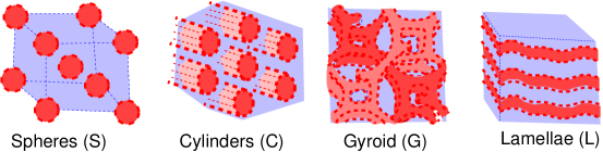
Figure 3.3: Self-assembled copolymer mesophases.

Nowadays, the theory of structure formation in polymer blends has reached a highly advanced level and theoretical calculations have predictive power, e.g., with respect to structures that can be expected in new polymeric materials. In this section, I shall present some of the most successful theoretical approaches.

III.1 Flory Huggins Theory

I begin with sketching the Flory-Huggins theory, which is the classical theory of phase separation in polymer blends, and which in some sense lays the foundations for all later, more sophisticated theories of polymer mixtures.

III.1.1 Basic Model for Binary Blends

We consider a binary blend of homopolymers A and B with length $N_{A}$ and $N_{B}$, and volume fractions $\Phi_{A}$ and $\Phi_{B}$. According to Flory [1] and Huggins [2], the free energy per monomer is approximately given by

$$\frac{f_{{}_{FH}}}{k_{{}_{B}}\!T}=\frac{\Phi_{A}}{N_{A}}\ln(\Phi_{A})+\frac{\Phi_{B}}{N_{B}}\ln(\Phi_{B})+\chi\Phi_{A}\Phi_{B}$$ (3.12)

with $\Phi_{A}+\Phi_{B}=1$. The first two terms account for the mixing entropy of the two components, and the last term for the (in)compatibility of the monomers. The parameter $\chi$ is the famous ’Flory Huggins parameter’, which will be discussed in more detail below. The generalization of this expression to ternary ABC homopolymer blends etc. is straighforward, one only needs to introduce several $\chi$-parameters $\chi_{AB}$, $\chi_{BC}$, and $\chi_{AC}$. Here we will only discuss binary systems.

By minimizing the free energy, Eq. (3.12), one easily identifies the region in phase space where the mixture phase separates into an A-rich phase and a B-rich phase. At low values of $\chi$, the blend remains homogeneous. Demixing sets in at a critical value $2\chi_{c}=(1/\sqrt{N_{A}}+1/\sqrt{N_{B}})^{2}$ for the critical composition $\Phi_{A,c}=1/(1+\sqrt{N_{A}/N_{B}})$. The region of stability of the homogeneous (mixed) blend is delimited by the ”binodal” line (see Fig. 3.4). Beyond the binodal, the homogeneous blend may still remain metastable. It becomes unstable at the ”spinodal”, which is defined as the line where the second derivative of $f_{{}_{FH}}$ in Eq.  (3.12) with respect to $\Phi_{A}$ vanishes. An example of a phase diagram with a binodal and a spinodal is shown in Fig. 3.4 (left). Fig. 3.4 (right) demonstrates the shift of the binodal with varying chain length ratio $N_{A}/N_{B}$.

The Flory-Huggins free energy, Eq. (3.12), was originally derived based on a lattice model, but it can also be applied to off-lattice systems. It does, however, rely on three critical assumptions:

• The polymer conformations are taken to be those of ideal chains, independent of the composition (ideality assumption, cf. Sec. II.4.2).

• The melt is taken to be incompressible, and monomers A and B occupy equal volumes.

• Local composition fluctuations are neglected (mean-field assumption).

In reality, none of these assumptions is strictly valid. The polymer conformations do depend on the composition, most notably for chains of the minority component. The incompressibility assumption is reasonable, but the volumes per monomer are not equal. As a consequence, the $\chi$-parameter is not a fixed parameter (at fixed temperature), but depends on the composition of the blend (see Sec. III.1.3). Finally, the composition fluctuations shift phase boundaries and may even fundamentally change the phase behavior. (see  Sec. III.2.5).

Figure 3.4: Left: Phase diagram for a binary AB polymer blend with B-chains twice as long as A-chains according to the Flory-Huggins theory. Thick solid line shows the binodal line (i.e., the demixing line), thin dashed line the spinodal line (i.e., the line where the homogeneous blend becomes unstable). Right: Binodals for binary AB blends with different chain length ratios as indicated.

III.1.2 Inhomogeneous Systems: Flory-Huggins-de Gennes Theory

Eq. (3.12), only describes homogeneous systems. The simplest approach to generalizing the Flory-Huggins theory to inhomogeneous systems, e.g., polymer blends containing interfaces, consists in adding a penalty on composition variations $(\nabla\Phi_{A})^{2}=(\nabla\Phi_{B})^{2}$. The coefficient of the square gradient term can be derived within a more advanced mean-field treatment, the random phase approximation, which will be described further below (Sec. III.3.1). One obtains the Flory-Huggins-de Gennes free energy functional for polymer blends,

$${\cal F}_{\mbox{\tiny FHdG}}[\Phi_{A}({\bf r})]=\rho_{0}\int{\rm d}{\bf r}\left\{f_{{}_{FH}}(\Phi_{A}({\bf r}))+\frac{k_{{}_{B}}\!T}{36}\big{(}\frac{b_{A}^{2}}{\Phi_{A}}+\frac{b_{B}^{2}}{\Phi_{B}}\big{)}(\nabla\Phi_{A})^{2}\right\}$$ (3.13)

(with $\Phi_{B}=1-\Phi_{A}$), where $b_{A}$ and $b_{B}$ are the Kuhn lengths of the homopolymers A and B, and $f_{{}_{FH}}(\Phi_{A}))$ is given by Eq. (3.12). The functional (3.13) can be applied if composition variations are weak, and have characteristic length scales of the order of the gyration radius of the chains (’weak segregation regime’, see Sec. III.3.1).

A very similar functional can be derived in the opposite case, where A- and B- polymers are fully demixed and separated by narrow interfaces. In this ’strong segregation’ regime, the blend can be described by the functional (see Sec. III.3.2)

$${\cal F}_{\mbox{\tiny SSL}}[\Phi_{A}({\bf r})]=\rho_{0}\int{\rm d}{\bf r}\left\{\chi\Phi_{A}\Phi_{B}+\frac{k_{{}_{B}}\!T}{24}\big{(}\frac{b_{A}^{2}}{\Phi_{A}}+\frac{b_{B}^{2}}{\Phi_{B}}\big{)}(\nabla\Phi_{A})^{2}\right\}.$$ (3.14)

At strong segregation, the mixing entropy terms in $f_{\mbox{\tiny FH}}$, Eq. (3.12), can be neglected, hence the functionals (3.13) and (3.14) are identical except for the numerical prefactor of the square gradient term. In the strong segregation limit, the square gradient penalty results from an entropic penalty on A and B segments due to the presence of the interface, whereas in the weak segregation limit, it is caused by the deformation of whole chains.

III.1.3 Connection to Reality: The Flory-Huggins Parameter

In the Flory-Huggins theory, the microscopic features of the blend are incorporated in the single Flory-Huggins parameter $\chi$. Not surprisingly, this parameter is very hard to access from first principles.

In the original Flory-Huggins lattice model, $\chi$ is derived from the energetic interactions between monomers that are neighbors on the lattice. The interaction energy between monomers $i$ and $j$ is taken to be characterized by energy parameters $\epsilon_{ij}$. The $\chi$-parameter is then given by

$$\chi=\frac{z-2}{2k_{{}_{B}}\!T}(2\epsilon_{AB}-\epsilon_{AA}-\epsilon_{BB})$$ (3.15)

where $z$ is the coordination number of the lattice. It is reduced by two ($z-2$) in order to account for the fact that interactions between neighbor monomers on the chain are fixed and have no influence on the demixing behavior.

In reality, the situation is not as simple. The miscibility patterns in real blends tend to deviate dramatically from that predicted by the Flory-Huggins model. Several blends exhibit a lower critical point instead of an upper critical point, indicating that the demixing is driven by entropy rather than enthalpy. The critical temperature $T_{c}$ of demixing often does not scale linearly with the chain length $N$, as one would expect from Eq. (3.15) (see Fig. 3.4). In blends of polystyrene and poly(vinyl methyl ether) (PS/PVME), for example, $T_{c}$ is nearly independent of $N$, and the critical concentration $\Phi_{c}$ is highly asymmetric even for roughly equal chain lengths, in apparent contrast with Fig. 3.4 ($N_{B}=N_{A}$) [33].

Formally, this problem can be resolved by arguing that the Flory-Huggins expression for $\chi$, Eq. (3.15), is oversimplified and that $\chi k_{{}_{B}}\!T$ is not a constant. Several factors contribute to the $\chi$-parameter, leading to a complex dependence on the temperature, the blend composition, and even the chain length.

Monomer incompatibility

: Monomers may be incompatible both for enthalpic and entropic reasons. For example, consider two nonpolar monomers $i$ and $j$. The van-der Waals attraction between them is proportional to the product of their polarizabilities $\alpha$, hence $\epsilon_{ij}\propto\alpha_{i}\alpha_{j}$ and $\chi\propto(\alpha_{A}-\alpha_{B})^{2}$. More generally, the enthalpic incompatibility of monomers $i$ and $j$ can be estimated by $\chi_{H}\propto(\delta_{A}-\delta_{B})^{2}$, where the $\delta_{i}$ are the Hildebrand solubility parameters of the components [34, 35]. In addition, entropic factors may contribute to the monomer incompatibility, which are, e.g., related to shape or stiffness disparities [36, 37, 38, 39, 40]. Since the enthalpic and entropic contributions evolve differently as a function of the temperature, the $\chi$-parameter will in general exhibit a complicated temperature dependence.

Equation-of-state effect

: In general, the volume per polymer depends on the composition of the blend. Already the volume per monomer is usually different for different monomer species; at constant pressure, $\chi$ therefore varies roughly linearly with $\Phi_{A}$ [41]. In blends of monomers with very similar monomer structure, e.g., isotopic blends, the linear contribution vanishes and a weak parabolic dependence remains, which can partly [42] (but not fully [43]) be explained by an ‘excess volume of mixing’.

Chain correlations

: Since the demixing is driven by intermolecular contacts, intramolecular contacts only contribute indirectly to the $\chi$-parameter. The estimate for $\chi$ can be improved if one replaces the factor $z-2$ by an ‘effective coordination number’ $z_{\mbox{\tiny eff}}$ which is given by the mean number of interchain contacts per monomer [44]. Moreover, the ideality assumption (see Sec. II.4.2) is not strictly valid. Chains in the minority phase (e.g., A chains in a B-rich phase) tend to shrink in order to reduce unfavorable contacts [45]. Since the segregation is effectively driven by $\chi N$, $\chi$ slightly depends on the chain length $N$ as a result. The situation becomes even more complex if copolymers are involved, which assume dumbbell shapes even in a disordered environment [46, 47]. This also may affect the effective $\chi$-parameter [48].

Composition correlations

: The effective interactions between monomers change if the local environment is not random. We have already noted earlier that the composition may fluctuate. Large-scale fluctuations can be incorporated in the Flory-Huggins framework in terms of a fluctuating field theory (see Secs. III.2.5 and III.3.1). Fluctuations (correlations) on the monomeric scale renormalize the $\chi$-parameter (nonrandom mixing). Moreover, the local fluid structure may depend on the local composition $\Phi$ (nonrandom packing).

In view of these complications, establishing an exhaustive theory of the $\chi$-parameter remains a formidable task [37, 49, 50, 51, 52, 53, 54]. Even the reverse problem of designing simplified particle-based polymer models with a well-defined $\chi$-parameters turns out to be highly non-trivial [55]. The very concept of a $\chi$-parameter has been challenged repeatedly, e.g., by Tambasco et al. [56], who analyzed experimental data for a series of blends and found that their thermodynamic behavior can be related to a single ‘$g-1$-parameter’, which is independent of composition, temperature and pressure. They suggest that this parameter may be more appropriate to characterize blends than the $\chi$-parameter. However, it has to be used in conjunction with an integral equation theory, the BGY lattice theory by Lipson [57, 58, 59], which is much more involved than the Flory-Huggins theory especially when applied to inhomogeneous systems.

Freed and coworkers [60, 36, 37, 40] have proposed a generalized Flory-Huggins theory, the ’lattice cluster theory’, which provides a consistent microscopic theory for macroscopic thermodynamic behavior. In a certain limit (high pressure, high molecular weight, fully flexible chain), this theory reproduces a Flory-Huggins type free energy with an effective $\chi$-parameter [49]

$$\chi_{\mbox{\tiny eff}}=\frac{(r_{A}-r_{B})^{2}}{z^{2}}+\chi_{0}\big{(}1-\frac{2(p_{A}\Phi_{A}+p_{B}\Phi_{B})}{z(z-2)}\big{)},$$ (3.16)

where $\chi_{0}$ is given by Eq. (3.15) and the parameters $r_{j}$, $p_{j}$ depend on the structure of the monomers $j$. Dudowicz et al. have recently pointed out that this model can account for a wide range of experimentally observed miscibility behavior [38, 39].

Another pragmatic and reasonably successful approach consists in using $\chi$ as a heuristic parameter. Assuming that it is at least independent of the chain length, it can be determined experimentally, e.g., from fitting small-angle scattering data to theoretically predicted structure factors [61, 62, 63]. Alternatively, $\chi$ can be estimated from atomistic simulations [64, 55]. The results from experiment and simulation tend to compare favorably even for systems of complex polymers [65].

III.2 Self-consistent Field Theory

I have taken some care to discuss the Flory-Huggins theory because it establishes a framework for more general theories of polymer blends. In particular, it provides the concept of the Flory-Huggins parameter $\chi$, which will be taken for granted from now on, and taken to be independent of the composition, despite the question marks raised in the previous section (Sec. III.1.3). In this section, I present a more sophisticated mean-field approach, the self-consistent field (SCF) theory. It was first proposed by Helfand and coworkers[66, 67, 68, 69, 70] and has since evolved to be one of the most powerful tools in polymer theory. Reviews on the SCF approach can be found, e.g., in Refs. [71, 72, 8].

III.2.1 How it works in principle

For simplicity, I will first present the SCF formalism for binary blends, and discuss possible extensions later. Our starting point is the Edwards Hamiltonian for Gaussian chains, Eq. (3.4), with a Flory-Huggins interaction term,

$${\cal H}_{I}[\hat{\rho}_{A},\hat{\rho}_{B}]/k_{{}_{B}}\!T=\rho_{0}\>\chi\>\int{\rm d}{\bf r}\>\hat{\Phi}_{A}\hat{\Phi}_{B}$$ (3.17)

where we have defined the ’monomer volume fractions’ $\hat{\Phi}_{j}=\hat{\rho}_{j}/\rho_{0}$ and incompressibility is requested, i.e., $\hat{\Phi}_{A}+\hat{\Phi}_{B}\equiv 1$ everywhere. The quantity $\hat{\rho}_{j}$ depends on the paths ${\bf R}_{\alpha}$ of chains of type $j$ and has been defined in Eq. (3.10).

We consider a mixture of $n_{A}$ homopolymers A of length $N_{A}$ and $n_{B}$ homopolymers B of length $N_{B}$ in the volume $V$. The canonical partition function is given by

$${\cal Z}=\frac{1}{n_{A}!n_{B}!}\left[\prod_{\alpha}\rho_{0}\int{\cal D}{\bf R}_{\alpha}\>e^{-{\cal H}_{G}[{\bf R}_{\alpha}]/kBT}\right]e^{-\rho_{0}\chi\int{\rm d}{\bf r}\>\hat{\Phi}_{A}\hat{\Phi}_{B}}\>\delta(\hat{\Phi}_{A}+\hat{\Phi}_{B}-1).$$ (3.18)

The product $\alpha$ runs over all chains in the system, $\rho_{0}\!\!\int{\cal D}{\bf R}_{\alpha}$ denotes the path integral over all paths ${\bf R}_{\alpha}(s)$, and we have introduced the factor $\rho_{0}$ in order to make ${\cal Z}$ dimensionless.

The path integrals can be decoupled by inserting delta-functions $\int{\cal D}{\rho}_{j}\>\delta(\rho_{j}-\hat{\rho}_{j})$ (with $j=$A,B), and using the Fourier representations of the delta-functions $\delta(\rho_{j}-\hat{\rho}_{j})=\int_{i\infty}{\cal D}W_{j}\>e^{\frac{1}{N}W_{j}(\rho_{j}-\hat{\rho}_{j})}$ and $\delta({\rho}_{A}+{\rho}_{B}-\rho_{0})=\int_{i\infty}{\cal D}\xi\>e^{\frac{1}{N}\>\xi({\rho}_{A}+{\rho}_{B}-\rho_{0})}.$ Here $N$ is some reference chain length, and the factor $1/N$ is introduced for convenience. This allows one to rewrite the partition function in the following form:

$${\cal Z}\propto\int_{i\infty}{\cal D}W_{A}\>{\cal D}W_{B}\>{\cal D}\xi\int_{\infty}{\cal D}\rho_{A}\>{\cal D}\rho_{B}\>e^{-{{\cal F}}/{k_{{}_{B}}\!T}}$$ (3.19)

with

$$\frac{{\cal F[W_{A},W_{B},\xi,\rho_{A},\rho_{B}]}_{\mbox{\tiny}}}{k_{{}_{B}}\!T} = \frac{\rho_{0}}{N}\>\Big{\{}\>\chi N\!\int{\rm d}{\bf r}\>\Phi_{A}\Phi_{B}-\sum_{j=A,B}\int\!{\rm d}{\bf r}\>W_{j}\Phi_{j}$$

$$\quad-\int\!{\rm d}{\bf r}\>\xi\>(\Phi_{A}+\Phi_{B}-1)-\!\sum_{j=A,B}V_{j}\>\frac{N}{N_{j}}\>\ln(\rho_{0}\>\frac{{\cal Q}_{j}}{n_{j}})\Big{\}},$$

($\Phi_{j}=\rho_{j}/\rho_{0}$), where $V_{j}$ denotes the partial volume occupied by all polymers of type $j$ in the system, and the functional

$${\cal Q}_{j}=\int{\cal D}{\bf R}\>e^{-{\cal H}_{G}[{\bf R}]/k_{{}_{B}}\!T}\>\>e^{-\frac{1}{N}\int_{0}^{N_{j}}{\rm d}s\>W_{j}({\bf R}(s))}.$$ (3.21)

is the partition function of a single, noninteracting chain $j$ in the external field $W_{j}$. Thus the path integrals are decoupled as intended, and the coupling is transferred to the integral over fluctuating fields $W_{j}$ and $\xi$.

Now the self-consistent field approximation consists in replacing the integral (3.19) by its saddle point, i.e., minimizing the effective Hamiltonian ${\cal H}$ with respect to the variables $\rho_{j}({\bf r})$ and $W_{j}({\bf r})$. The minimization procedure results in a set of equations,

$$\begin{array}[]{rclcccl}\langle\hat{\Phi}_{j}\rangle&=&\Phi_{j}&&\mbox{with}&&j=\mbox{A,B}\\ W_{j}&=&\chi N\langle\hat{\Phi}_{i}\rangle-\xi&&\mbox{with}&&i,j=\mbox{A,B}\quad\mbox{and}\quad i\neq j,\end{array}$$ (3.22)

where $\langle\hat{\Phi}_{j}\rangle$ denotes the average of $\hat{\Phi}_{j}$ in a system of noninteracting chains subject to the external fields $W_{j}({\bf r})$. One should note that the latter are real, according to Eq. (3.22), even though the original integral (3.19) is carried out over the imaginary axis. Intuitively, the $W_{j}({\bf r})$ can be interpreted as the effective mean fields acting on monomers due to the interactions with the surrounding monomers. Together with the incompressibility constraint, the equations (3.22) form a closed cycle which can be solved self-consistently.

For future reference, we note that it is sometimes convenient to carry out the saddle point integral only with respect to the variables $W_{j}({\bf r})$. This defines a free energy functional ${\cal F}_{\mbox{\tiny SCF}}[\Phi_{A}]$, which has essentially the same form as ${\cal F}$ (Eq. III.2.1), except that the variables $W_{\alpha}({\bf r})$ and $\xi({\bf r})$ are now real Lagrange parameter fields that enforce $\langle\hat{\Phi}_{A}\rangle=\Phi_{A}$, $\langle\hat{\Phi}_{B}\rangle=\Phi_{B}$, and $\Phi_{B}=1-\Phi_{A}$ and depend on $\Phi_{A}$. The same functional can also be derived by standard density functional approaches, using as the reference system a gas of non-interacting Gaussian chains [73].

In some cases, one would prefer to operate in the grand canonical ensemble, i.e., at variable polymer numbers $n_{j}$. The resulting SCF theory is very similar. The last term in Eq. (III.2.1) is replaced by $(-\sum_{j}z_{j}{\cal Q}_{j})$, where $z_{j}$ is proportional to the fugacity of the polymers $j$.

The formalism can easily be generalized to other inhomogeneous polymer systems. The application of the theory to multicomponent A/B/C/… homopolymer blends with a more general interaction Hamiltonian ${\cal H}_{I}[\hat{\rho}_{A},\hat{\rho}_{B},\hat{\rho}_{C},\cdots]$ replacing Eq. (3.17) is straightforward. The self-consistent field equations (3.22) are simply replaced by

$$W_{j}=\frac{N}{k_{{}_{B}}\!T}\>\frac{\delta{\cal H}_{I}[\{\rho_{i}\}]}{\delta\rho_{j}}-\xi.$$ (3.23)

If copolymers are involved, the single-chain partition function ${\cal Q}_{c}$ for the corresponding molecules must be adjusted accordingly. For example, the single-chain partition function for an A:B diblock copolymer of length $N_{c}$ with A-fraction $f$ reads

$${\cal Q}_{c}=\int{\cal D}{\bf R}\>e^{-{\cal H}_{G}[{\bf R}]/k_{{}_{B}}\!T}\>\>e^{\frac{1}{N}\int_{0}^{fN_{c}}{\rm d}s\>W_{A}({\bf R}(s))+\frac{1}{N}\int_{fN_{c}}^{N_{c}}{\rm d}s\>W_{B}({\bf R}(s))}.$$ (3.24)

The general SCF free energy functional for incompressible multicomponent systems is given by

$$\frac{{\cal F}_{\mbox{\tiny SCF}}[\{\rho_{j}\}]}{k_{{}_{B}}\!T} = \frac{{\cal H}_{I}[\{\rho_{i}\}]}{k_{{}_{B}}\!T}-\sum_{j}\frac{1}{N}\int{\rm d}{\bf r}\>W_{j}\>\rho_{j}-\frac{1}{N}{\rm d}{\bf r}\>\xi(\sum_{j}\rho_{j}-\rho_{0})$$ (3.25)

$$-\sum_{\alpha}n_{\alpha}\>\ln(\rho_{0}\>\frac{{\cal Q}_{\alpha}}{n_{\alpha}}),$$

where the sum $j$ runs over monomer species and the sum $\alpha$ over polymer types.

The SCF theory has been extended in various ways to treat more complex systems, e.g., compressible melts and solutions [74, 75], macromolecules with complex architecture [76], semiflexible polymers [77] with orientational interactions [78, 79], charged polymers[80], polydisperse systems[81, 82], polymer systems subject to stresses [83, 84], systems of polymers undergoing reversible bonds [85, 86], or polymer/colloid composites [87, 88, 89].

III.2.2 How it works in practice

In the previous section, we have derived the basic equations of the SCF theory. Now I describe how to solve them in practice. The first task is to evaluate the single-chain partition functions ${\cal Q}_{j}$ and the corresponding density averages $\langle\hat{\rho}_{j}\rangle$ for noninteracting chains in an external field.

We consider a single ideal chain of length $N$ in an external field $W({\bf r},s)$, which may not only vary in space ${\bf r}$, but also depend on the monomer position $s$ in the chain in the case of copolymers. It is convenient to introduce partial partition functions

$$q({\bf r},s) = \int\!\!{\cal D}{\bf R}\>\>e^{-{\cal H}_{G}[{\bf R}]/k_{{}_{B}}\!T}\>\>e^{\frac{1}{N}\int_{0}^{s}{\rm d}s^{\prime}\>W({\bf R}(s^{\prime}),s^{\prime})}\>\delta({\bf R(s)}-{\bf r}),$$ (3.26)

$$q^{\dagger}({\bf r},s) = \int\!\!{\cal D}{\bf R}\>\>e^{-{\cal H}_{G}[{\bf R}]/k_{{}_{B}}\!T}\>\>e^{\frac{1}{N}\int_{0}^{s}{\rm d}s^{\prime}\>W({\bf R}(s^{\prime}),N-s^{\prime})}\>\delta({\bf R(s)}-{\bf r}),$$ (3.27)

where the path integrals ${\cal D}{\bf R}$ are carried out over paths of length $s$. According to the Feynman-Kac formula [90], the functions $q({\bf r},s)$ and $q^{\dagger}({\bf r},s)$ satisfy a diffusion equation

$$\frac{\partial}{\partial s}\>q({\bf r},s) = (\frac{b^{2}}{6}\Delta-\frac{W({\bf r},s)}{N})\>q({\bf r},s)$$ (3.28)

$$\frac{\partial}{\partial s}\>q^{\dagger}({\bf r},s) = (\frac{b^{2}}{6}\Delta-\frac{W({\bf r},N-s)}{N})\>q^{\dagger}({\bf r},s)$$ (3.29)

with the initial condition $q({\bf r},0)=q^{\dagger}({\bf r},0)=1$. Numerical methods to solve diffusion equations are available[91], hence $q$ and $q^{\dagger}$ are accessible quantities. The single-chain partition function can then be calculated via

$${\cal Q}=\int{\rm d}{\bf r}\>q({\bf r},N)=\int{\rm d}{\bf r}\>q^{\dagger}({\bf r},N)$$ (3.30)

and the distribution of the $s$th monomer in space is $q({\bf r},s)\>q^{\dagger}({\bf r},N-s)/{\cal Q}$.

More specifically, to study binary homopolymer blends, one must solve the diffusion equations for the partial partition functions $q_{j}=q^{\dagger}_{j}$ in an external field $W=W_{j}$ (with $j=$ A,B). The averaged volume fractions of monomers $j$ are then given by

$$\langle\hat{\Phi}_{j}({\bf r})\rangle=\frac{1}{\rho_{0}}\>\frac{n_{j}}{{\cal Q}_{j}}\int_{0}^{N_{j}}{\rm d}s\>q_{j}({\bf r},s)\>q^{\dagger}_{j}({\bf r},N-s).$$ (3.31)

in the canonical ensemble, and

$$\langle\hat{\Phi}_{j}({\bf r})\rangle=\frac{z_{j}}{N}\>\int_{0}^{N_{j}}{\rm d}s\>q_{j}({\bf r},s)\>q^{\dagger}_{j}({\bf r},N-s)$$ (3.32)

in the grand canonical ensemble. If AB diblock copolymers with fraction $f$ of A-monomers are present, one must calculate the partial partition functions $q_{c}$ and $q^{\dagger}_{c}$ in the external field $W({\bf r},s)=W_{A}$ for $s<fN_{c}$ and $W({\bf r})=W_{B}$ for $s\geq fN_{c}$. The contribution of the copolymers to the volume fraction $\langle\hat{\Phi}_{A}\rangle$ is $n_{C}/\rho_{0}{\cal Q}_{C}\>f_{A}({\bf r})$ with $f_{A}({\bf r})=\int_{0}^{fN_{c}}{\rm d}s\>q_{C}({\bf r},s)q_{C}^{\dagger}({\bf r},N-s)$ in the canonical ensemble, and $z_{c}/Nf_{A}({\bf r})$ in the grandcanonical ensemble.

With this recipe at hand, one can calculate the different terms in Eqs. (3.22). The next problem is to solve these equations simultaneously, taking account of the incompressibility constraint. This is usually done iteratively. I refer the reader to Section 3.4. in Ref. 91 for a discussion of different iteration methods.

III.2.3 Application: Diblock Copolymer Blends, Part I

To illustrate the power of the SCF approach, I cite one of its most spectacular successes: The reproduction of arbitrarily complex copolymer mesophases. In a series of seminal papers, Matsen and coworkers have calculated phase diagrams for diblock copolymer melts[92, 93]. Fig. 3.5 compares an experimental phase diagram due to Bates and coworkers [94, 95, 96] with the SCF phase diagram of Matsen and Bates [93]. The SCF theory reproduces the experimentally observed structures. At high values of $\chi N$ (‘strong segregation’) the SCF phase diagram features the correct sequence of mesophases at almost the correct value of the fraction of A-monomers $f$. At low values of $\chi N$ (’weak segregation’), the two phase diagrams are distinctly different. This can be explained by the effect of fluctuations and will be discussed further below (Secs. III.2.5 and IV.4.2, see also Fig. 3.8).

  

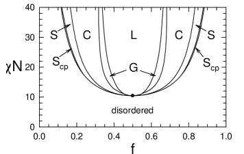
Figure 3.5: Experimental phase diagram for polystyrene-polyisoprene diblock copolymer melts (left, after Refs. 94, 95, 96) compared with phase diagram obtained with the SCF theory by Matsen and coworkers (right, after Ref. 93) in the coordinates $\chi N$ and A block volume fraction $f$. The labels S,C,L, and G correspond to the structures shown in Fig. 3.3. In addition, the SCF phase diagram features a close-packed sphere phase S_cp. All phase transitions are first order except for the disordered/lamellar-transition at $f=1/2$ in the SCF phase diagram. Courtesy of Mark W. Matsen, adapted from M.W. Matsen, J. Phys.: Cond. Matter 14, R21 (2002).

Tyler and Morse have recently reconsidered the SCF phase diagram and predicted the existence of yet another mesophase, which has an orthorombic unit cell and an Fddd structure and intrudes in a narrow regime at the low $\chi N$-end of the gyroid phase [97]. This phase was later indeed found in a polystyrene-polyisoprene diblock copolymer melt by Takenaka and coworkers [98].

III.2.4 Related Mean-Field Approaches

So far, I have focussed on sketching a variant of the SCF theory which was originally developed by Helfand and coworkers [70]. A number of similar approaches have been proposed in the literature.

Scheutjens and Fleer have developed a SCF theory for lattice models[99], which is applied very widely [6]. Scheutjens-Fleer calculations are very efficient and incorporate in a natural way the finite (nonzero) range of monomer interactions. To account for this in the Helfand theory, one must introduce additional terms in (3.9) [69, 70], which indeed turn out to become important in the vicinity of surfaces[75].

Carignano and Szleifer[100] have proposed a SCF theory where chains are sampled as a whole in a surrounding mean field. Hence intramolecular interactions are accounted for exactly and the chain statistics corresponds to that of self-avoiding walks (Sec. II.4.1). This approach is more suitable than the standard SCF theory to study polymers in solution, or melts of molecules with low-molecular weight, where the ideality assumption (see Sec. II.4.2) becomes questionable [101].

In this chapter, I have chosen a field-theoretic way to present the SCF theory. Freed and coworkers [102, 73] have derived the same type of theory from a density functional approach, using a reference system of non-interacting Gaussian chains. Compared to the density functional approach, the field-theoretic approach has the advantage that the effect of fluctuations can be treated in a more transparent way (see Sec. III.2.5). On the other hand, information on the local liquid structure of the melt, (i.e., monomer correlation functions, packing effects etc.), can be incorporated more easily in density functional approaches [103, 104]. Density functionals have also served as a starting point for the development of dynamical theories which allow to study the evolution of multiphase polymer blends in time [105, 106, 107, 108] (see Sec. IV.3.2).

III.2.5 Fluctuation Effects

Mean-field approaches for polymer systems like the SCF theory tend to be quite successful, because polymers overlap strongly and have many interaction partners. However, there are several instances where composition fluctuations become important and may affect the phase behavior qualitatively.

To illustrate some of them, we show the phase diagram of ternary mixtures containing A and B homopolymers and AB diblock copolymers in Fig. 3.6. The left graph shows the experimental phase diagram [109], the right graph theoretical phase diagrams obtained by Düchs et al [110, 111] from the SCF theory (solid lines) and from field-based computer simulations (dashed line, see Sec. IV.2.3 for details on the simulation method). Regions where different types of fluctuations come into play are marked by I – IV.

• Fluctuations are important in the close vicinity of critical points, i.e., continuous phase transitions. They affect the values of the critical exponents, which characterize e.g., the behavior of the specific heat at the transition [90]. In Fig. 3.6, such critical transitions are encountered at high homopolymer concentration, where the system essentially behaves like a binary A/B mixture with a critical demixing point. This point belongs to the Ising universality class, hence the system should exhibit Ising critical behavior. It has to be noted that in polymer blends, critical exponents typically remain mean-field like until very close to the critical point[112, 113, 114].

• The effect of fluctuations is more dramatic in the vicinity of order-disorder transitions (ODT), e.g., the transition between the disordered phase and the lamellar phase at low homopolymer concentrations. Fluctuations destroy the long-range order in weakly segregated periodic structures, they shift the ODT and change the order of the transition from continuous to first order (Brazovskii mechanism [115, 116]). This effect accounts for the differences between the experimental and the SCF phase diagram in Fig. 3.5.

• The SCF phase diagram features a three-phase (Lamellar + A + B) coexistence region reaching up to a Lifshitz point. Lifshitz points are generally believed to be destroyed by fluctuations in three dimensions.

• In strongly segregated mixtures, fluctuations affect the large-scale structure of interfaces. Whereas mean-field interfaces are flat, real interfaces undulate. The so-called ’capillary waves’ may destroy the orientational order in highly swollen lamellar phases. A locally segregated, but globally disordered ’microemulsion’ state intrudes between the homopolymer-poor lamellar phase and the homopolymer-rich two-phase region in Fig. 3.6.

Both in the cases of III) and IV), the effect of fluctuations is to destroy lamellar order in favor of a disordered state. However, the mechanisms are different. This is found to leave a signature in the structure of the disordered phase, which is still locally structured with a characteristic wavevector $q^{*}$ [111]. In the Brazovskii regime, the wavevectore $q^{*}$ corresponds to that calculated from the SCF theory (defect driven disorder regime, $D\mu E$). In the capillary wave regime, the characteristic length scale increases, compared to that calculated from the SCF theory (genuine microemulsion regime, $G\mu E$).

  

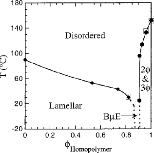
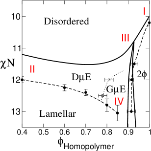
Figure 3.6: Experimental phase diagram for symmetric ternary blends of PDMS+PEE+PDMS-PEE ($N_{C}\sim 5N_{H}$) featuring lamellar phase, phase-separated region $2\Phi$, and microemulsion channel $B\mu E$ (left, from Ref. 109), compared with theoretical phase diagrams (right) from SCF theory (solid lines) and Monte Carlo simulations at $C=50$ (dashed lines/circles). The dotted lines separate disordered regions with different local structure: $D\mu E$, defect driven disorder, and $G\mu E$, genuine microemulsion morphology. The regions I-IV are discussed in the text. Left Figure: Reprinted with permission from M.A. Hillmyer, W.W. Maurer, T.P. Lodge, F.S. Bates, K. Almdal, J. Phys. Chemistry B 103, 4814 (1999). Reproduced by permission of the Royal Society of Chemistry. Right Figure: Adapted from Refs. 110, 111 (Düchs et al 2003 and 2004).

Formally, the effect of fluctuations is hidden in the overall prefactor $\rho_{0}/N$ in the SCF Hamiltonian ${\cal H}$ (Eq. 3.25). The larger this factor, the more accurate is the saddle point integration that lies at the heart of the SCF approximation. One can thus define a ’Ginzburg parameter’ $C=R_{g}^{d}\rho_{0}/N$, which characterizes the strength of the fluctuations. Here the factor $R_{g}^{d}$ must be introduced to make $C$ dimensionless ($d$ is the spatial dimension), and $R_{g}=Nb^{2}/6$ is the natural length scale of the system, the radius of gyration of an ideal chain of length $N$. The Ginzburg parameter roughly corresponds to the ratio of the volume spanned by a chain, $R_{g}^{d}$, and the volume actually occupied by a chain, $N/\rho_{0}$, and thus measures the degree of interdigitation of chains. At $C\to\infty$, the SCF approximation becomes exact. The numerical simulations shown in Fig. 3.6 were carried out at $C=50$ (using the length of the copolymers as the reference length), which still seems large. Nevertheless, the effect of fluctuations is already quite dramatic.

In three dimensions ($d=3$), the Ginzburg parameter is proportional to the square root of the chain length, $\sqrt{N}$. This is why the mean-field theory becomes very good for systems of polymers with high molecular weight, and only fails at selected points in the phase diagram. The relation $C\propto\sqrt{N}$ has motivated the definition of an ’invariant polymerization index’ $\bar{N}=Nb^{6}\rho_{0}^{2}\propto C^{2}$, which is also often used to quantify fluctuation effects [72, 91]. In two dimensional systems, $C$ is independent of the chain length and fluctuation effects are much stronger. Furthermore, topological constraints become important (i.e., the fact that chains cannot cross each other) which are not included in the Helfand model. In three dimensional systems of linear polymers, they only affect the dynamics (leading to reptation), but in two dimensions, they also change the static properties qualitatively [15].

Finally, we note that fluctuations can also be treated to some extent within the SCF theory, by looking at Gaussian fluctuations about the SCF solution[117]. This is useful for calculating structure factors and carrying out stability analyses. However, Gaussian fluctuations alone cannot bring about the qualitative changes in the phase behavior and the critical exponents which have been described above.

III.3 Analytical Theories

The SCF equations have to be solved numerically, which can be quite challenging from a computational point of view. In addition, they also serve as a starting point for the derivation of simpler approximate theories, which may even have analytical solutions in certain limits.

Two main regimes have to be distinguished here. In the weak segregation limit, $\chi N$ is small, and the A and B homopolymers or copolymer blocks are barely demixed. This is the realm of the ’random phase approximation’ (RPA), which can be derived systematically from the SCF theory. In the strong segregation limit, $\chi N$ is large, the polymers or copolymer blocks are strongly demixed and the system can basically be characterized in terms of its internal interfaces.

III.3.1 Weak Segregation and Random Phase Approximation

We first consider the situation at low $\chi N$. In this case, the composition varies smoothly, A-rich domains still contain sizeable fractions of B-monomers and vice versa, and the interfaces between domains are broad, i.e., their width is comparable to the radius of gyration of the chains.

The idea of the RPA is to perform a systematic expansion about a homogeneous reference state. More precisely, we use the SCF free energy density functional, Eq. (3.25), as a starting point, and then expand ${\cal F}$ about the homogeneous state. Defining $\Phi_{A}=\rho_{A}/\rho_{0}$ as usual, using $\Phi_{A}+\Phi_{B}\equiv 1$, and introducing the Fourier representation $\Phi({\bf k})=\int{\rm d}{\bf r}\>e^{i{\bf kr}}\Phi({\bf r})$, we obtain a functional of the form

$${\cal F}_{\mbox{\tiny RPA}}[\Phi_{A}({\bf r})] = V\>\rho_{0}\>f_{\mbox{\tiny homo}}+k_{{}_{B}}\!T\>\frac{\rho_{0}}{N}\>\Big{\{}\>\frac{1}{2V}\sum_{{\bf k}\neq 0}|\Phi_{A}({\bf k})|^{2}\>\Gamma_{2}({\bf k})$$ (3.33)

$$\frac{1}{6V^{2}}\sum_{{\bf k},{\bf k}^{\prime}\neq 0}\Phi_{A}({\bf k})\Phi_{A}({\bf k}^{\prime})\Phi_{A}(-{\bf k}-{\bf k}^{\prime})\>\Gamma_{3}({\bf k},{\bf k}^{\prime})+\cdots\Big{\}},$$

where $f_{\mbox{\tiny homo}}$ is the SCF free energy per chain in the reference system, and the coefficient $\Gamma_{n}$ depend on the direct monomer interactions and on the intrachain correlations of free ideal Gaussian chains.

We focus on the leading coefficient. To calculate $\Gamma_{2}$ for a given blend, we define the pair correlators $K_{ij}$ [117, 71]

$$K_{ij}({\bf k})=\langle\hat{\rho}_{i}({\bf k})\hat{\rho}_{j}({\bf k})\rangle\>\frac{1}{\rho_{0}N},$$ (3.34)

which give the density-density correlations in an identical blend of noninteracting, ideal Gaussian chains and can thus be expressed in terms of Debye functions $g_{{}_{D}}\!(x)$ (Eq. (3.7)). For example, for binary blends of homopolymers with chain length $N_{j}$, gyration radii $R_{g,j}$, and mean volume fractions $\bar{\Phi}_{j}$ ($j$=A,B), the pair correlators are given by

$$K_{AA}=\frac{N}{N_{A}}\bar{\Phi}_{A}g_{{}_{D}}\!(k^{2}R_{g,A}^{2}),\quad K_{BB}=\frac{N}{N_{B}}\bar{\Phi}_{B}g_{{}_{D}}\!(k^{2}R_{g,B}^{2}),\quad K_{AB}=K_{BA}=0$$ (3.35)

For pure diblock copolymer blends with A-fraction $f$, one gets

$$\begin{array}[]{c}K_{AA}=f^{2}g_{{}_{D}}\!(f\>k^{2}R_{g}^{2})\qquad K_{BB}=(1-f)^{2}g_{{}_{D}}\!((1-f)\>k^{2}R_{g}^{2})\\ K_{AB}=\frac{1}{2}\Big{(}g_{{}_{D}}\!(k^{2}R_{g}^{2})-f^{2}g_{{}_{D}}\!(fk^{2}R_{g}^{2})-(1-f)^{2}g_{{}_{D}}\!((1-f)k^{2}R_{g}^{2})\Big{)}.\end{array}$$ (3.36)

Having calculated $K_{ij}$, one can evaluate $\Gamma_{2}$ according to [117, 71]

$$\Gamma_{2}=\Big{(}\frac{K_{AA}+K_{BB}+K_{AB}+K_{BA}}{K_{AA}K_{BB}-K_{AB}K_{BA}}-2\chi N\Big{)}.$$ (3.37)

The function $\Gamma_{2}$ is particularly interesting, because it is directly related to the structure factor of the homogeneous phase, $S({\bf k})\propto\Gamma_{2}({\bf k})^{-1}$. Hence the RPA provides expressions for structure factors which can be compared to small angle scattering experiments, e.g., to determine effective interaction parameters. This is probably its most important application.

We will now discuss specifically the application of the RPA to binary homopolymer blends and to diblock copolymer blends.

(i) Binary homopolymer blends and Flory-Huggins-de Gennes functional

According to Eqs. (3.35) and (3.37), the RPA coefficient $\Gamma_{2}$ for binary blends is given by

$$\Gamma_{2}({\bf k})=\Big{(}\frac{N/N_{A}}{\bar{\Phi}_{A}\>g_{{}_{D}}\!(k^{2}R_{g,A}^{2})})+\frac{N/N_{B}}{\bar{\Phi}_{B}\>g_{{}_{D}}\!(k^{2}R_{g,B}^{2})})-2\chi N\Big{)}.$$ (3.38)

We assume that the composition varies only slowly in the system (on length scales not much shorter than $R_{g}$), and expand $\Gamma_{2}$ for small wave vectors. Using $g_{{}_{D}}\!(x)\approx 1-x/3$ and $R_{g,j}^{2}=b_{j}^{2}N_{j}/6$, and inserting our result in the RPA expansion (3.33), we obtain the free energy functional

$${\cal F}_{\mbox{\tiny RPA}}[\Phi_{A}] \approx V\>\rho_{0}\>f_{\mbox{\tiny homo}}+k_{{}_{B}}\!T\>\rho_{0}\>\Big{\{}\>\frac{1}{2V}\sum_{{\bf k}\neq 0}(\frac{1}{\bar{\Phi}_{A}N_{A}}+\frac{1}{\bar{\Phi}_{B}N_{B}}-2\chi)|\Phi_{A}({\bf k})|^{2}$$ (3.39)

$$\qquad+\>\frac{1}{2V}\sum_{{\bf k}\neq 0}\frac{1}{18}(\frac{b_{A}^{2}}{\bar{\Phi}_{A}}+\frac{b_{B}^{2}}{\bar{\Phi}_{B}})|\Phi_{A}({\bf k})|^{2}\>k^{2}\Big{\}}.$$

The first two terms in (3.39) correspond to the second order expansion of the integral $\rho_{0}\int{\rm d}{\bf r}\>f_{\mbox{\tiny SCF}}(\Phi_{A})$, where $f_{\mbox{\tiny SCF}}(\Phi_{A})$ is the SCF free energy per chain in a homogeneous system with A-volume fraction $\Phi_{A}$. It thus seems reasonable to replace them by the full integral. The last term is a square gradient term in real space. Together, one recovers the Flory-Huggins-de Gennes functional of Sec. III.1.2, Eq. (3.13).

(ii) Copolymer melts, Leibler theory, and Ohta-Kawasaki functional

In diblock copolymer blends, Eqs. (3.36) and (3.37) yield the RPA coefficient

$$\Gamma_{2}({\bf k})=\Big{(}\frac{G(1)}{G(f)G(1-f)-(G(1)-G(f)-G(1-f))^{2}/4}-2\chi N\Big{)}$$ (3.40)

with the short hand notation $G(f)=f^{2}g_{{}_{D}}\!(fk^{2}R_{g}^{2})$. At low $\chi N$, $\Gamma_{2}({\bf k})$ is positive. Upon increasing $\chi N$, one encounters a spinodal line where $\Gamma_{2}({\bf k})$ becomes zero for some nonzero $k=q^{*}$, and the disordered state becomes unstable with respect to an ordered microphase separated state.

Since the function $\Gamma_{2}({\bf k})$ is spherically symmetric in ${\bf k}$, it does not favor a specific type of order. The information on possible ordered states is contained in the higher order coefficients $\Gamma_{n}$, most notably, in the structure of the cubic term, $\Gamma_{3}$. In a seminal paper of 1979, Leibler has carried out a fourth order RPA expansion and deduced a phase diagram which already included the three copolymer phases L, C, and S (Fig. 3.3) [118]. Milner and Olmsted later showed that the Leibler theory is also capable of reproducing the gyroid phase [119]. The RPA phase diagram roughly coincides with the full SCF phase diagram, as established 1996 by Matsen and Bates [93], up to $\chi N<12$. Unfortunately, fluctuations have a massive effect on the phase diagram at these small $\chi N$ (see Fig. 3.5), therefore the predictive power of the Leibler theory must be questioned. Nevertheless, it is useful for identifying potential ordered phases and phase transitions in copolymer systems. Generalized Leibler theories still prove to be efficient tools to analyze phase transitions in complex copolymer blends by analytical considerations [120].

Next we attempt to construct a simplified free energy functional for diblock copolymer melts, in the spirit of the Flory-Huggins-de Gennes functional. To this end, we again expand $\Gamma_{2}$ in powers of ${\bf k}$, as in (i). Compared to homopolymer blends, however, there is an important difference: $\Gamma_{2}({\bf k})$ has a singularity at ${\bf k}\to 0$ and diverges according to

$$\Gamma_{2}({\bf k})\approx\frac{3}{2f^{2}(1-f)^{2}}\>\frac{1}{k^{2}R_{g}^{2}}\qquad\mbox{at}\qquad k\to 0.$$ (3.41)

The singularity accounts for the fact that large-scale composition fluctuations are not possible in copolymer blends, since the A- and B- blocks are permanently linked to each other. It ensures that the structure factor $S({\bf k})$, vanishes at ${\bf k}\to 0$, suppresses macrophase separation and is thus ultimately responsible for the onset of microphase separation in the RPA theory.

A $1/k^{2}$ term like (3.41) in a density functional corresponds to a long-range Coulomb type interaction. This observation motivated Ohta and Kawasaki [121] in 1986 to propose a free energy functional for copolymer melts, which combines a regular square-gradient functional accounting for direct short-range interactions with a long-range Coulomb term accounting for the connectivity of the copolymers. In real space, the Ohta-Kawasaki functional has the form

$${\cal F}_{\mbox{\tiny OK}}[\Phi_{A}]=\frac{\rho_{0}}{N}\int\!\!{\rm d}{\bf r}\>\Big{\{}{\cal W}(\Phi_{A})+\frac{B}{2}(\nabla\Phi_{A})^{2}\Big{\}}+\frac{\rho_{0}}{N}\>\frac{A}{2}\int\!\!{\rm d}{\bf r}\>{\rm d}{\bf r}^{\prime}\>{\cal G}({\bf r},{\bf r^{\prime}})\>\delta\Phi_{A}({\bf r})\>\delta\Phi_{A}({\bf r}^{\prime})$$ (3.42)

with $\delta\Phi_{A}({\bf r})=\Phi_{A}({\bf r})-\bar{\Phi}_{A}$. The last term introduces the long-range interactions, with $G({\bf r},{\bf r}^{\prime})$ defined such that

$$\Delta{\cal G}({\bf r},{\bf r}^{\prime})=-\delta({\bf r}-{\bf r}^{\prime}),$$ (3.43)

which corresponds to ${\cal G}({\bf r},{\bf r}^{\prime})\sim 1/|{\bf r}-{\bf r}^{\prime}|$ in infinitely extended systems.

Given Eq. (3.41), it seems natural to identify $A=3/(2f^{2}(1-f)^{2}R_{g}^{2})$. The choice of ${\cal W}$ and $B$ is somewhat more arbitrary. The function ${\cal W}(\Phi_{A})$ is a free energy density with two degenerate minima and can be approximated by a fourth order polynomial in $\Phi_{A}$. As for the coefficient of the square gradient term, $B$, Ohta and Kawasaki originally estimated it from the asymptotic behavior of $\Gamma_{2}$ at $k\to\infty$,

$$\Gamma_{2}({\bf k})\approx\frac{1}{2f(1-f)}\>{k^{2}R_{g}^{2}}\qquad\mbox{at}\qquad k\to\infty,$$ (3.44)

which yields $B=R_{g}^{2}/(2f(1-f))$. Later, they noted that this choice of $B$ gives the wrong interfacial width at stronger segregation, which has implications for the elastic constants and the equilibrium period of the ordered phases, and suggested to replace $B$ by a constant in the strong segregation limit [122].

The Ohta-Kawasaki functional reproduces microphase separation and complex copolymer phases such as the gyroid phase [123, 124] and even the Fddd phase [124]. It can be handled much more easily than the Leibler theory or the full SCF theory (see Sec. IV.3.2), therefore it is particularly popular in large-scale dynamical simulations of copolymer melts (see Sec. IV.3.2). Different authors have generalized it to ternary blends containing copolymers [125, 126, 123]. In particular, Uneyama and Doi have recently proposed a general density functional for polymer/copolymer blends that reduces to the Flory-Huggins-de Gennes functional in the homopolymer case and to the Ohta-Kawasaki functional in the diblock case.

III.3.2 Strong Segregation

I turn to discussing the situation at high $\chi N$. The A-rich and B-rich (micro)phases are then well-separated by sharp interfaces. The free energy contribution from the interfacial regions (i) and the chain conformations inside the A- or B- domains (ii) can be treated separately.

(i) Interfacial profiles and ground state dominance

In the interfacial region, the free energy is dominated by the contribution of the direct A-B interactions and the local stretching of segments. Chain end effects can be neglected. This simplifies the situation considerably.

We first note that the diffusion equation ((3.28) or (3.29)) for a $j$-chain or a $j$-block of a chain has the same structure than the time-dependent Schrödinger equation, if one identifies $s\leftrightarrow it$. As is well known from quantum mechanics, the general solution can formally be expressed as [127] $q_{j}({\bf r},s)=\sum_{n}c_{n}\psi_{n,j}({\bf r})e^{-\epsilon_{n,j}s}$, where $\{\psi_{n,j}({\bf r}),\epsilon_{n,j}\}$ are Eigenfunctions and Eigenvalues of the operator $(b_{j}^{2}/6\>\Delta-W_{j}({\bf r})/N)$. At large $s$, the smallest Eigenvalue $\epsilon_{0,j}$ dominates, i.e., $q_{j}({\bf r},s)\propto\psi_{0,j}({\bf r})e^{-\epsilon_{0,j}s}$, and the resulting density in the large $N_{j}$ limit is $\rho_{j}\propto|\psi_{0,j}|^{2}e^{-\epsilon_{0,j}N_{j}}$. This type of approximation is called ’ground state dominance’. It is commonly used to study polymers at interfaces and surfaces.

In the case of blends, we have the freedom to shift the fields $W_{j}({\bf r})$ by a constant value, hence we can set $\epsilon_{0,j}=0$. The self-consistent field equations can thus be written as

$$\rho_{j}=\rho_{0}\>|\psi_{j}({\bf r})|^{2}\quad\mbox{with}\quad(\frac{b_{j}^{2}}{6}\Delta-\frac{W_{j}}{N})\>\psi_{j}=0\quad\mbox{and}\quad W_{j}=\frac{N}{k_{{}_{B}}\!T}\>\frac{\delta{\cal H}_{I}}{\delta\rho_{j}}-\xi,$$ (3.45)

where $\psi_{j}$ is normalized such that ${\cal Q}_{j}=\int{\rm d}{\bf r}\>|\psi_{j}({\bf r}|^{2}=V_{j}$ is the partial volume occupied by the polymers $j$, and $\xi({\bf r})$ ensures $\sum_{j}|\psi_{j}|^{2}\equiv 1$.

In order to derive an epression for the free energy, we first note that Eqs. (3.45) minimize a Lagrange action,

$${\cal L}={\cal H}_{I}+\frac{k_{{}_{B}}\!T}{6}\>\rho_{0}\>\int{\rm d}{\bf r}\>(b_{A}^{2}(\nabla\psi_{A})^{2}+b_{B}^{2}(\nabla\psi_{B})^{2}),$$ (3.46)

with respect to $\psi_{j}$ under the constraint $|\psi_{A}|^{2}+|\psi_{B}|^{2}\equiv 1$. One easily checks that ${\cal L}$ vanishes for homogeneous bulk states, and that the minimized ${\cal L}$ is equal to the extremized SCF Hamiltonian ${\cal F}_{\mbox{\tiny SCF}}$, Eq. (3.25) up to a constant. Hence ${\cal L}$ can be identified with the interfacial free energy. Rewriting it in terms of the volume fractions $\phi_{j}$ and using $(\nabla\Phi_{A})^{2}=(\nabla\Phi_{B})^{2}$, one obtains the free energy functional

$${\cal F}_{\mbox{\tiny int}}[\Phi_{A}({\bf r})]={\cal H}_{I}+\rho_{0}\int{\rm d}{\bf r}\>\>\frac{k_{{}_{B}}\!T}{24}(\frac{b_{A}^{2}}{\Phi_{A}}+\frac{b_{B}^{2}}{\Phi_{B}})(\nabla\Phi_{A})^{2},$$ (3.47)

which reproduces Eq. (3.14) for Flory-Huggins interactions (3.17).

For $b_{A}=b_{B}=b$ and Flory-Huggins interactions, the self-consistent field equations (3.45) are solved by a $\tanh$ profile, $(\rho_{A}-\rho_{B})\sim\rho_{0}\tanh(z/w_{\mbox{\tiny SSL}})$ with the interfacial width $w_{\mbox{\tiny SSL}}=b/\sqrt{6\chi}$ and the interfacial tension $\sigma_{\mbox{\tiny SSL}}=k_{{}_{B}}\!T\rho_{0}b\sqrt{\chi/6}$ [66, 67, 68].

(ii) Copolymer conformations and strong stretching theory

The free energy functional (3.47) is sufficient to describe strongly segregated homopolymer blends. In copolymer blends, additional contributions come into play due to the fact that the copolymer junctions are confined to the interfaces and the copolymer blocks stretch away from them into their respective A or B domains. The associated costs of configurational free energy can be estimated within a second approximation scheme, the ’strong stretching’ theory (SST) [128, 129, 130, 131].

The main idea of the SST was put forward in 1985 by Semenov[128], who noted that for strongly stretched copolymer blocks, the paths fluctuate around a set of ’most probable paths’. This motivates to approximate the single-chain partition function ${\cal Q}$, Eq. (3.21), by its saddle point, i.e., the path integral in ${\cal Q}$ is replaced by an integral over ’classical’ paths ${\bf R}_{c}$ that extremize the integrand and thus satisfy the differential equation [132]

$$\frac{3}{b^{2}}\>\frac{{\rm d}^{2}{\bf R}_{c}}{{\rm d}s^{2}}=\frac{1}{N}\>\nabla W({\bf R}).$$ (3.48)

We will treat the copolymer blocks as independent chains of length $M$. The classical paths corresponding to one block are then characterized by their boundary conditions, ${\bf R}_{c}(0)={\bf r}_{j}$ and ${\bf R}_{c}(M)={\bf r}_{e}$, where the junction ${\bf r}_{j}$ is confined to an interface and the free end ${\bf r}_{e}$ is distributed everywhere in its domain.

Next, we note that for infinitely long blocks, the classical paths must satisfy

$${\rm d}{\bf R}_{c}/{\rm d}s|_{s=M}=0\qquad\mbox{for}\quad M\to\infty$$ (3.49)

at the free end. Mathematically speaking, they would not have a well-defined end position otherwise. Physically speaking, the ’average’ chain representing the classical path does not sustain tension at the free end, which seems reasonable. In the following, Eq. (3.49) is also imposed for finite (large) blocks as an additional boundary condition. Eq. (3.48) is then overdetermined and can, in general, no longer be solved for arbitrary end positions ${\bf r}_{e}$. To ensure that chain ends are indeed free to move throughout the domain, the field $W({\bf r})$ must have a special shape. Specifically, near flat interfaces it must be parabolic as a function of the distance $z$ from the interface [129, 130],

$$\frac{1}{N}W(z)=-\frac{3}{8}\>\frac{\pi^{2}}{b^{2}M^{2}}z^{2}.$$ (3.50)

This is one of the main results of the SST. It generally applies to situations where strongly stretched polymers are attached to an interface, e.g., strongly segregated copolymer blocks [133, 72], or polymer brushes in solvents of arbitrary quality [131]. The SST field must always have the form (3.50), and the remaining task is to realize this by a suitable choice of the chain end distribution $P({\bf r}_{e})$. In the incompressible blend case, $P({\bf r}_{e})$ must be chosen such that the density in the domains is constant, $\rho_{0}$.

Luckily, we do not have to evaluate $P({\bf r}_{e})$ explicitly to calculate the free energy. The SST field has another convenient property: One can show that the stretching energy of classical paths of fixed length $N$ in a field satisfying Eqs. (3.48) and (3.49) is exactly equal to the negative field energy,

$$\int_{0}^{N}{\rm d}s\>\frac{3}{2b^{2}}\Big{(}\frac{{\rm d}{\bf R}_{c}}{{\rm d}s}\Big{)}^{2}=-\frac{1}{N}\int_{0}^{N}{\rm d}s\>W({\bf R}_{c}(s)).$$ (3.51)

Summing over all blocks in a domain, the total stretching energy is thus given by

$$\frac{{\cal F}_{\mbox{\tiny stretch}}}{k_{{}_{B}}\!T}=-\frac{1}{N}\int{\rm d}{\rm r}\>\rho({\bf r})\>W({\bf r})\approx\rho_{0}\frac{3}{8}\>\frac{\pi^{2}}{b^{2}M^{2}}\int{\rm d}{\bf r}\>z^{2},$$ (3.52)

where the integral is over the volume of the domain, and $z$ denotes the closest distance to an interface. The total energy of the system can be estimated as the sum over the stretching energies in the different domains, Eq. (3.52), and the interfacial energy, Eq. (3.47), and then used to evaluate the relative stability of different phases. In the strong segregation limit, only the C, L, and S phase are found to be stable [72], in agreement with SCF calculations at high $\chi N$.

The validity of the strong stretching theory seems to be restricted to very large chains [134]. This is presumably to a large extent due to the requirement (3.49), which does not necessarily hold for classical paths of finite length. Netz and Schick [135, 136] have shown that an unrestricted ’classical theory’, which just builds on the saddle point integration of ${\cal Q}$ and avoids using (3.49), gives results that agree better with the SCF theory. However, the classical theory has to be solved numerically, and the computational advantage over the full SCF theory is not evident.

The SST has found numerous applications [72] and has been extended and improved in various respect. It provides an analytical approach to analyzing multicomponent polymer blends in a segregation regime where the SCF theory becomes increasingly cumbersome, due to the necessity of handling narrow interfaces.

III.4 An Application: Interfaces in Binary Blends

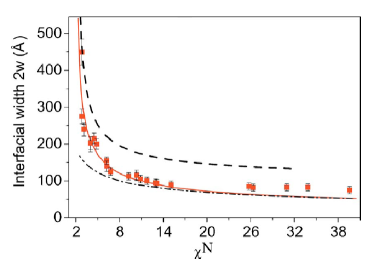
Figure 3.7: Intrinsic width of interfaces between A- and B-phases in binary polyolefin blends as a function of $\chi N$, compared with the predictions of the weak segregation theory (long dashed line), the strong segregation theory (dot dashed line), and the full SCF theory (solid line). From Ref. 137.

To close the theory section, I discuss the simplest possible examples of an inhomogeneous polymer system: An interface in a symmetrical binary homopolymer blend. This system has been studied intensely in experiments [138, 139, 140, 141, 142, 143, 137]. By mixing random copolymers of ethylene and ethyl-ethylene with two different, but very well defined copolymer ratios, Carelli et al. [143, 137] were able to tune the Flory-Huggins parameter very finely and study interfacial properties in a wide range of $\chi N$ between the weak segregation limit and the strong segregation limit. Fig. 3.7 compares the results for the interfacial width and compares them with the mean-field prediction for the weak segregation limit, the strong segregation limit, and the full numerical result.

We should note that there is a complication here. As mentioned earlier, fluid-fluid interfaces are never flat, they exhibit capillary waves [144, 145]. This leads to an apparent broadening of the interfacial width $w$ [146]. The apparent width depends on the lateral length scale of the observation $L$ and can be calculated according to [147, 148]

$$w^{2}=w_{0}^{2}+\frac{k_{{}_{B}}\!T}{4\sigma}\>\ln\Big{(}\frac{L}{a_{0}}\Big{)}\quad\mbox{or}\quad w^{2}=w_{0}^{2}+\frac{2k_{{}_{B}}\!T}{\pi\sigma}\>\ln\Big{(}\frac{L}{a_{0}}\Big{)},$$ (3.53)

depending how it is measured. Here $w_{0}$ is the ’intrinsic’ width, $\sigma$ the interfacial tension, and $a_{0}$ a ’coarse-graining length’, which is roughly given by the interfacial width [146, 148]. Both the quantities $L$ and $a_{0}$ are not very well defined in an actual experiment. Fortunately, they only enter logarithmically, therefore the result is not very sensitive to their values. The theoretical curves shown in Fig. 3.7 include the capillary wave broadening, calculated using the interfacial tension from the respective theory.

Comparing the curves in Fig. 3.7, one finds that the weak segregation theory consistently overestimates the width, and the strong segregation theory consistently underestimates it. The numerical SCF values interpolate between the two regimes and are in excellent quantitative agreement with the experimental data over almost the whole range of $\chi N$. The SCF theory is also found to perform very well compared to computer simulations [149, 148]. It reproduces many features of the interfacial structure, such as chain end distributions, local segment orientations etc. at a quantitative level, if capillary waves are accounted for [148], This illustrates the power of the SCF theory to describe the local structure of inhomogeneous polymer systems, even if the global structure is affected by large-scale composition fluctuations.

IV Simulations of Multiphase Polymer Systems

Whereas theoretical work on multiphase polymer systems has a long-standing tradition, the field of simulations in this area is much younger. This is because polymer simulations are computationally very expensive, which has essentially rendered them unfeasible until roughly 20 years ago. In this section, I will attempt to give an overview over the current state-of-the-art of simulations of inhomogeneous multicomponent polymer systems.

IV.1 Coarse-Graining, Part II

One of the obvious challenges in multiphase polymer simulations is that polymers are such big molecules, which moreover self-organize into even larger supramolecular structures. Polymeric materials exhibit structure on a wide range of length scales, from the atomic scale up to micrometers. Their specific material properties are to a great extent determined by local inhomogeneities and internal interfaces, and depend strongly on the interplay between these mesostructures in space and time. In order to understand the materials and make useful predictions for new substances, one must analyze their properties on all time and length scales of interest. Therefore, multiscale modeling has become one of the big topics in computational polymer science.

The central element of multiscale modeling is coarse-graining. By successively eliminating degrees of freedom (electronic structure, atomic structure, molecular structure, etc.), a hierarchy of models is constructed (see Sec. II.2). For each type of model, optimized simulation methods are developed, which allow one to investigate specific aspects of the materials.

Having identified suitable classes of coarse-grained models, one can proceed in two different manners:

Generic Modeling

This approach has been favored historically, and up to date, the overwhelming majority of simulations of multicomponent polymer systems is still based on it (see Sec. IV.4). Generic models are simple and computationally efficient. They are not designed to represent specific materials; rather, they are the simulation counterpart of the theoretical models discussed in the previous section. They are suited to study generic properties of polymer and copolymer systems, i.e., to identify the behavior that can be expected from their stringlike structure, their chemical incompatibility etc. Simulations of generic models are also particularly suited to test theories.

Generic models are used in all areas of materials science, and in most cases, they only give qualitative insights into the behavior of a material. This is different for polymers, because of their universal properties (see Sec. II). For example, we have already seen in Fig. 3.7 that a generic theoretical model (the Edwards model) quantitatively predicts important aspects of the interfacial structure in real polymer melts.

Nevertheless, the predictive power of generic models is restricted, and relies on the knowledge of ’heuristic’ parameters such as the $\chi$-parameter. Therefore, a second approach is attracting growing interest.

Systematic Bottom-Up Modeling

The idea of systematic coarse-graining is to establish a hierarchy of models for the same specific material, starting from an ab-initio description, with well-defined quantitative links between the different levels.

Ideally, the goal is to replace many degrees of freedom by a selection of fewer ’effective’ degrees of freedom. If one is only interested in equilibrium properties, the problem is at least well-defined. For each possible coarse-grained configuration, one must evaluate a partial partition function of the full system under the constraints imposed by the values of the coarse-grained degrees of freedom. This procedure results in an effective potential in the coarse-grained space, which is, in general, a true multibody potential – it cannot be separated into contributions of pair potentials. If one is interested in dynamical properties, the situation is even more complicated. One must replace a dynamical system for all variables by a lower dimensional system for a subset of effective variables. This can be done approximately, e.g., using Mori Zwanzig projector operator techniques [150]. The new dynamical system is inevitably a stochastic process with memory, i.e., the future time evolution not only depends on the current state of the system, but also on its entire history.

Obviously, such ’ideal coarse-graining’ is not feasible for polymer systems. Instead, researchers adopt a heuristic approach, where they first define a coarse-grained model, which typically has no memory and only pair potentials, and match the properties of the coarse-grained model with those of the fine-grain model as good as they can: The model parameters are chosen such that the coarse-grained model reproduces physical properties of interest, such as correlation functions or diffusion constants [151, 152, 153, 154].

Already early on, researchers have started to develop schemes for mapping real polymers on lattice models [155, 156, 157]. Nowadays, off-lattice models are more common. Early approaches focussed on the task of reproducing the correct intrachain correlations by optimizing the bond potentials in the chains [155]. Later, the interchain correlations were considered as well, which can be matched by adjusting the non-bonded, intermolecular potentials in the coarse-grained model. It is important to note that the resulting effective potentials depend on the concentration and the temperature [158] (much like the $\chi$-parameter itself). Different methods to determine effective potentials have been devised and even automated packages are available [153, 159, 160, 161, 162]. The reverse problem – how to reconstruct a fine-scale model from a given coarse-scale configuration – has also been addressed [163, 164]. Nowadays, the available techniques for mapping static properties are relatively advanced. In contrast, the field of mapping dynamical properties is still in its infancy [165].

The standard multiscale approach is sequential, i.e., numerical simulations are carried out separately for different levels. Currently, increasing effort is devoted to developing hybrid schemes where several coarse-graining levels are considered simultaneously within one single simulation [166, 167].

Despite the large amount of work that has already been devoted to systematic coarse-graining, coarse-grained simulation studies of realistic multicomponent polymer blends are still scarce. Mattice and coworkers have carried out lattice simulations of blends containing polyethylene and polypropylene homopolymers and copolymers [168, 169, 170]. Faller et al have developed and studied a coarse-grained model for blends of polyisoprene and polystyrene [171, 172, 173].

IV.2 Overview of structural models

After these general remarks, I shall give a brief overview over the different models that are currently used in multicomponent polymer simulations.

IV.2.1 Atomistic Models

Atomistic simulations are computationally intensive, and rely very much on the quality of the force fields. (Force fields are a separate issue in multiscale modeling, which shall not be discussed here.) Therefore, atomistic simulations of blends are still relatively scarce. So far, most studies have focussed on miscibility aspects [174, 175, 176, 177, 178, 179, 180, 181, 182, 183, 184]. Already early on, atomistic and mesoscopic simulations were combined in multiscale studies: Atomistic simulations were used to determine the Flory-Huggins $\chi$-parameter, coarse-grained methods were then applied to study large-scale aspects of phase separation [185, 186, 187, 188, 189, 190, 191] or mesophase formation [192]. Only few fully atomistic studies deal with aspects beyond miscibility, e.g, the formation of lamellar structures in diblock copolymers [193], or the diffusion of small molecules in blends [194].

IV.2.2 Coarse-Grained Particle Models

The coarse-grained models for polymers can be divided into two main classes: Coarse-grained particle models operate with descriptions of the polymers that are considerably simplified, compared to atomistic models, but still treat them as explicit individual objects. Field models describe polymer systems in terms of spatially varying continuous fields. I begin with discussing some of the most common particle models.

Lattice Chain Models

Lattice models have the oldest tradition among the coarse-grained particle models for polymer simulations, and are still very popular. The first molecular simulations of multiphase polymer systems – studies of binary homopolymer blends by Sariban and Binder in 1987[195, 196] and by Cifra and coworkers in 1988 [197] – were based on lattice models. They are particularly suited to be studied with Monte Carlo methods, and several smart Monte Carlo algorithms have been designed especially for lattice polymer simulations [198, 199].

In molecular lattice models, the polymers are represented as strings of monomers confined to a lattice. A natural approach consists in placing the ’monomers’ on lattice sites and linking them by bonds that connect nearest-neighbor sites. For many applications, it has proven useful to apply less rigid constraints on the links and allow for bonds of variable length, which may also connect second-nearest neighbors [200] or stretch over even longer distances [201]. Moreover, the lattice is usually not entirely filled with monomers, but also contains a small fraction of voids. This is because most Monte Carlo algorithms for polymers do not work at full filling, and special algorithms have to be devised for that case[202]. One particularly popular lattice model is the ’bond-fluctuation model’, devised in 1988 by Carmesin and Kremer [203]. It is based on the cubic lattice; monomers do not occupy single sites, but entire cubes in a cubic lattice. They are connected by ’fluctuating bonds’ of varying length, ($2,\sqrt{5},\sqrt{6},3$ or $\sqrt{10}$ lattice constants). In the bond-fluctuation model, a polymer system behaves like a dense polymer melt already at the volume fraction $0.5$. Therefore, it can be simulated very efficiently.

Despite their intrinsically anisotropic character, lattice models are able to reproduce most known self-assembled mesophases in copolymer melts, even the gyroid phase in diblock copolymers [204]. Nowadays, they are used to study such complex systems as ABC triblock copolymer melts confined in cylindrical nanotubes [205], which feature a rich spectrum of novel morphologies, e.g., stacked disks, curved lamellar structures, and various types of helices.

Off-Lattice Chain Models

For many years, only lattice simulations were sufficiently efficient that they could be used to study polymer blends at a molecular level. With computers becoming more and more powerful, off-lattice chain models become increasingly popular. Compared to lattice models, they have the advantage that they provide easy access to forces and can also be used in Molecular Dynamics or Brownian Dynamics simulations. They do not impose restrictions on the size and shape of the simulation box (in lattice models, the box dimensions have to be multiple integers of the lattice constant). The structure of space is not anisotropic as in lattice models. Whereas the inherent anisotropy of lattice models does not seem to cause problems if the lattice model is sufficiently flexible and if the chains are sufficiently long, simulations of shorter chains can be hampered by lattice artifacts.

In bead-spring models, polymers are represented by chains of spherically symmetric force centers connected by springs. Numerous variants have been proposed, which differ in the choice of the spring potentials (the bonded interactions) and the choice of the pairwise interactions between the beads (the non-bonded potentials).

The simplest choice of spring potential is a harmonic potential. In order to prevent chains from crossing each other in dynamical simulations, an anharmonic cutoff on the spring length is often imposed. A popular choice is the ’Finitely Extensible Nonlinear Elastic’ (FENE) potential

$$V_{\mbox{\tiny FENE}}(b)=\frac{k}{2}\>d^{2}\>\ln\Big{(}1-\frac{(b-b_{0})^{2}}{d^{2}}\>\Big{)},$$ (3.54)

which reduces to a harmonic spring potential with equilibrium spring length $b_{0}$ at $b\approx b_{0}$, and diverges at $|b-b_{0}|\to d$. In some applications, the springs are constrained to have fixed lengths – however, this requires the use of special algorithms and changes slightly the distribution of bond angles [198]. In addition, some bead-spring models also include bending potentials that allow one to tune the chain stiffness, or even torsional potentials.

The non-bonded interactions drive the segregation of the monomers. As we have discussed in Sec. III.1.3, both energetic and entropic factors can contribute to making monomers incompatible. Many models operate with energetic monomer (in)compatibilities, but models with entropically driven segregation are also common. As an example, we consider one commonly used type of potential, the truncated Lennard-Jones potentials

$$V_{\mbox{\tiny LJ}}(r)=\epsilon\Big{(}(\sigma/r)^{12}-(\sigma/r)^{6}+C\Big{)}\quad\mbox{for}\quad r<r_{c}$$ (3.55)

($V_{\mbox{\tiny LJ}}=0$ otherwise), where the parameter $C$ is chosen such that $V_{\mbox{\tiny LJ}}(r)$ is continuous at $r=r_{c}$. If the cutoff parameter $r_{c}$ is larger than $2^{1/6}\sigma$ (a common choice is $r=2.5\sigma$), the potential has a repulsive core surrounded by an attractive well . In this case, energetic incompatibility can be imposed by using species dependent interaction parameters $\epsilon_{ij}$ with $2\epsilon_{AB}<\epsilon_{AA}+\epsilon_{BB}$. If the cutoff parameter is $r_{c}\leq 2^{1/6}$, the potential is purely repulsive. In this case, one can still enforce monomer segregation by choosing species dependent and non-additive interaction radii $\sigma_{ij}$ with $2\sigma_{AB}>\sigma_{AA}+\sigma_{BB}$. The mechanism driving the segregation is the Equation-of-State effect discussed in Sec. III.1.3. A simulation model that is based on this idea has been proposed by Grest, Lacasse and Kremer in 1996 [206]. It is more efficient than conventional models with energetically driven segregation, because the interaction range is shorter. We note that high pressures have to be applied to keep the chains together and to drive the demixing.

In the context of ’Dissipative particle dynamics’ (DPD) simulations, (see below) it has also become popular to use soft non-bonded potentials without a hard core. A typical DPD-potential has the form [207]

$$V_{\mbox{\tiny DPD}}(r)=\frac{v}{2}\>\Big{(}1-r/r_{c}\Big{)}^{2}\quad\mbox{for}\quad r<r_{c}$$ (3.56)

($V_{\mbox{\tiny DPD}}=0$ otherwise). Demixing is induced by using species dependent parameters $v_{ij}>0$ with $2v_{AB}>(v_{AA}+v_{BB})$. The mechanism driving the segregation is again related to the Equation-of-State effect – like particles overlap more strongly than unlike particles. The DPD simulation method was originally proposed in the context of fluid simulations, where every DPD particle supposedly represents a lump of true particles. This motivates the absence of hard, impenetrable cores and even a roughly linear shape [208]. Early on, DPD potentials were also used in polymer simulations [207]. As long as topological constraints are not important, the monomer potentials do not need to have a hard core (see also the discussion at the end of the next section).

’Edwards’ Models

A special class of chain models are the Edwards models, which shall be treated separately. The idea is to implement directly an Edwards-type interaction ${\cal H}_{I}$ (Eq. (3.9)) in a particle-based simulation. The molecules are modeled as off-lattice chains as before, and the non-bonded interactions are given by a potential $V={\cal H}_{I}[\{\rho_{i}\}]$ that depends on local monomer densities $\rho_{i}({\bf r})$. To complete the definition of the model, one must prescribe how to evaluate the local densities. This is most easily done by simply counting the monomers in each cell of a grid. Other prescriptions that do not impose a grid are also conceivable.

Edwards models are not yet very common in simulations of multiphase polymer systems, but they will very likely gain importance in the future. The basic idea was put forward by Zuckermann and coworkers [209, 210] in 1994 in the context of polymer brush simulations. It was first applied to studying microphase separation in block copolymers by Besold et al. [211], who also showed that the model produces correct single-chain behavior in solution [212] (i.e., the chains behave like regular self-avoiding chains). In the following, the power of the approach has been demonstrated in a series of impressive work by Müller and coworkers[213] (see also Sec. IV.3.1).

Two notes are in order here. First, it is difficult to impose strict incompressibility in particle-based simulations. Instead, dense melt simulations usually operate at finite compressibility: One introduces an additional term [66]

$${\cal H}_{I,\mbox{\tiny comp.}}=\frac{\kappa}{2}(\rho_{A}+\rho_{B}-\rho_{0})^{2}$$ (3.57)

with a high modulus $\kappa$ in the interaction Hamiltonian. Second, chains may overlap in the Edwards models. They share this ’problem’ with the DPD models introduced in the previous section. In three dimensions, the lack of hard core interactions has no effect on the static properties of linear polymers [212, 213]. Topological constraints become important in two dimensions [15], or in melts of cyclic polymers [214], or, most notably, when looking at dynamical properties. In Edwards models, chains do not entangle, and reptation dynamics has to be put in ’by hand’ [215].

Ellipsoid Model

In 1998, Murat and Kremer proposed a model that allows to study weakly segregated polymer blends on the scale of the gyration radius $R_{g}$ and beyond [216]. If details of the conformations are not of interest, the polymers can be replaced by single, soft particles with ellipsoidal shape. The idea was then pursued mainly by Eurich, Maass, and coworkers [217, 218, 219], who also suggested to extend the model to diblock copolymers by modeling them as dimers to account for their dumbbell shape [219]. Sambrisky and Guenza have recently worked out a microscopic foundation for coarse-graining diblock copolymers into such dumbbells, which is based on liquid-state integral equations [220].

IV.2.3 Field-Based Models

Field-based models for polymer systems no longer treat the molecules as individual objects, but describe them in terms of locally varying fluctuating fields. Among these, the molecular field theories still incorporate some information on the conformations of molecules, and the Ginzburg-Landau models focus on the large-scale structure only.

Field-Theoretical Models

Field-theoretical models are the molecular field equivalent of the particle-based ’Edwards’ models discussed above. The idea is to use the starting point of the self-consistent field theory, i.e., a field-theoretic expression for the partition function (e.g., Eq. (3.19)), and to evaluate the functional integrals over fluctuating fields by simulation methods. Since some fields are complex, one is confronted with a sign problem (the integrand oscillates between positive and negative). Fredrickson and coworkers have demonstrated that the integrals can nevertheless be evaluated in many cases using a method borrowed from elementary particle physics, the ’Complex Langevin’ simulation method [221, 8, 222]. We refer to Ref. 8 for a general presentation of the method, and Ref. 223 for technical details.

To be more specific, let us consider the system discussed in Sec. III.2.1, a blend of polymers/copolymers containing two types of monomers A and B, with Flory-Huggins interactions (3.17). Rather than evaluating the integral over all five fluctuating fields $W_{A,B},\xi,\rho_{A,B}$ in Eq. (3.19), we reconsider the original partition function, Eq. (3.18), and decouple the integrals over different paths (polymer conformations) by means of a Hubbard-Stratonovich transformation [90]. This is possible, because the interaction Flory-Huggins interaction ${\cal H}_{I}[\{\hat{\rho}_{i}\}]$ is quadratic in the densities $\hat{\rho}_{i}$. The result is a functional integral over ’only’ two fields – one which is conjugate to the total density $\hat{\rho}=\hat{\rho}_{A}+\hat{\rho}_{B}$ and imaginary, and one which is conjugate to the composition $\hat{m}=\hat{\rho}_{B}-\hat{\rho}_{A}$ and real:

$${\cal Z}\propto\int_{i\infty}{\cal D}W_{+}\int_{\infty}{\cal D}W_{-}\>e^{-{\cal F}_{\mbox{\tiny FTS}}/k_{{}_{B}}\!T}$$ (3.58)

with

$${\cal F}_{\mbox{\tiny FTS}}[W_{+},W_{-}]=\frac{\rho_{0}}{N}\Big{\{}\frac{1}{\chi N}\int{\rm d}{\bf r}\>W_{-}^{2}-\int{\rm d}{\bf r}\>W_{+}-\sum_{\alpha}V_{\alpha}\frac{N}{N_{\alpha}}\>\ln\big{(}\rho_{0}{\cal Q}_{\alpha}/n_{\alpha}\big{)}\>\Big{\}}.$$ (3.59)

This partition function is the starting point for field-theoretical simulations of incompressible AB (co)polymer systems.

The idea to study multiphase polymer systems by direct evaluation of fluctuating field integrals like Eq. (3.58) was first put forward by Ganesan and Fredrickson in 2001 [224]. They used Complex-Langevin simulations to look at fluctuation effects in pure symmetric diblocks. Since then, Fredrickson and coworkers have shown that the method can be extended in various ways, e.g., it can deal with external stresses [225]), and it can be applied very naturally to charged polymers [226, 227]. Nevertheless, there are still problems with it. The theoretical foundations of the Complex Langevin method are not fully established. One can show that under certain conditions, it produces the correct statistical averages if the system reaches equilibrium [8]. However, the stability of the simulations cannot be ensured. Even if the Langevin step size is chosen small, a fraction of simulation runs still crashes [223]. Such problems are unknown from other simulation methods. Since it is generally not widely used and very young in the polymer community, the Complex Langevin method still suffers from teething troubles.

An alternative approach to carrying out field-theoretical simulations in melts has been suggested by Düchs et. al. [110] (see also Ref. 91). They suggested to treat only the real integral over $W_{-}$ with computer simulation and approximate the problematic imaginary integral over $W_{+}$ by its saddle-point. The integral over $W_{-}$ can be evaluated by standard Monte Carlo methods. The results from this partial saddle point approach were shown to agree quantitatively with the full Complex Langevin simulation [110]. Possible strategies to improve upon the saddle point integral have been pointed out by Bäurle and coworkers [228, 229, 230].

As already pointed out, field-theoretic models are in some sense equivalent to particle-based Edwards models (if the latter use discrete Gaussian chain models). In field-theoretical simulations, the mean-field limit can be reached very naturally and at low computational cost. Hence they are more efficient than particle-based simulations at high polymer densities, close to the SCF limit, whereas particle-based simulations are superior at lower polymer densities.

An application of field-theoretic simulations was already shown in Sec. III.2.5. The simulation data shown in Fig. 3.6 were obtained with field-theoretic Monte Carlo simulations.

Molecular Density Functionals

Molecular density functionals are free energy functionals of the type (3.25). They are used in dynamical density functional simulations (see Sec. IV.3.2).

Ginzburg-Landau Models

Ginzburg-Landau models no longer incorporate specific information on chain conformations and thus have a much simpler structure than molecular field models. Examples are the Flory-Huggins-de Gennes functional for homopolymer blends (Eq. (3.13)), or the Ohta-Kawasaki functional for diblock copolymer melts (Eq. (3.42)). This is the highest level of coarse-graining discussed in the present article.

IV.3 Overview of Dynamical Models

In many cases, only static equilibrium properties are of interest, and then most dynamical models are equivalent. When looking at dynamical properties such as dynamical response functions, or at nonequilibrium situations, the choice of the dynamical model becomes relevant. In the following, I summarize some important models that have been used to study multiphase polymer systems.

IV.3.1 Particle-Based Dynamics

Kinetic Monte Carlo (MC)

A priori, the Monte Carlo (MC) method has been invented as a method to evaluate high dimensional integrals (i.e., thermal averages), and is designed for studying dynamics. Nevertheless, MC simulations are used for dynamical studies, based on the fact that like many static properties, dynamical phenomena are also often governed by universal principles. In kinetic MC simulations, one analyzes the artificial Monte Carlo evolution of a system in order to gain insight into real dynamical processes in the system. The main requirement is that the Monte Carlo moves are only local and reasonably ’realistic’, i.e., chain crossings are not allowed. Kinetic Monte Carlo simulations have been used, e.g., to study the early stages of demixing in binary blends or the ordering dynamics in block copolymer melts.

Molecular Dynamics (MD)

In Molecular Dynamics simulations, one solves directly Newton’s or Hamilton’s equations of motions. This is the most straightforward approach to studying dynamical processes in a system. As usual, of course, the devil is in the details [198].

Brownian Dynamics

In Brownian dynamics simulations, one also solves equations of motion, but the underlying dynamics is not Hamiltonian. As we have noted earlier (Sec. IV.1), systematic coarse-graining necessarily turns a dynamical system into a stochastic process. Brownian Dynamics simulations account for this fact. They include dissipative and stochastic forces, which supposedly represent the interaction of the coarse-grained degrees of freedom with those that have been integrated out. In general, however, these forces are not derived systematically from the original model, but postulated heuristically.

More specifically, the particles $j$ experience three types of forces:

$$m_{j}\ddot{\bf r}_{j}={\bf F}_{j}^{C}+{\bf F}_{j}^{D}+{\bf F}_{j}^{R}$$ (3.60)

The first term ${\bf F}_{j}^{C}$ correspondes to the conservative forces, which are derived from the interparticle potentials of the structural model under consideration. These forces also enter the standard Molecular Dynamics simulations. The second ${\bf F}_{j}^{D}$ term is a dissipative force that couples to the velocity of the particles. The last term ${\bf F}_{j}^{R}$ is a Gaussian stochastic force with mean zero whose amplitude is related to the dissipative force by a ’fluctuation-dissipation theorem’ [231]. In a canonical simulation, the last two terms constitute a thermostat, i.e., they maintain the system at a given temperature $T$. Microcanonical models where energy is randomly shifted between ’internal’ and ’external’ degrees of freedom have been designed as well.

In the simplest (canonical) Ansatz, the dissipative force on a particle $j$ at time $t$ is proportional to its velocity ${\bf v}_{j}(t)$. According to the fluctuation-dissipation theorem, the stochastic force then fulfills

$${\bf F}_{j}^{D}=-\gamma_{j}{\bf v}_{j}\qquad\longleftrightarrow\quad\langle F_{j,\alpha}^{R}(t)\>F_{k,\beta}^{R}(t^{\prime})\rangle=2\gamma_{j}\>k_{{}_{B}}\!T\>\delta_{\alpha\beta}\>\delta_{jk}\>\delta(t-t^{\prime}).$$ (3.61)

Other choices are possible. For example, the dissipative force on $j$ can depend on the velocities of other particles $k$ as well, and/or on the history of the system. The fluctuation-dissipation relation for the stochastic force has to be adjusted accordingly [231]. The dynamics defined by Eq. (3.61) is commonly used because it is so simple, but it has the disadvantage that it is not Galilean-invariant – a system moving at constant speed is treated differently than a system at rest. Therefore, it does not incorporate hydrodynamic effects correctly, and it is not suited to study nonequilibrium systems such as polymer melts in shear flow.

Dissipative Particle Dynamics (DPD)

The problems of Eq. (3.61) are avoided in the recently developed ’Dissipative Particle Dynamics’ (DPD) method [232, 233]. DPD is a special type of Brownian Dynamics which is Galilean-invariant and has become very popular in simulations of complex fluids in recent years. The dissipative and stochastic forces are constructed such that they conserve the total momentum and angular momentum in the system. Consequently, they couple to relative velocities of particles rather than absolute velocities, and they act as central forces (to preserve angular momentum). Specifically, the forces acting on a particle $j$ are given by

$${\bf F}_{j}^{C}-\sum_{k\neq j}\Big{\{}\gamma\>\omega(r_{jk})\>(\hat{\bf r}_{jk}{\bf v}_{jk})\>\hat{\bf r}_{jk}+\sqrt{2\gamma\>k_{{}_{B}}\!T\>\omega(r_{jk})}\>\hat{\bf r}_{jk}\>\zeta_{jk}\Big{\}},$$ (3.62)

where ${\bf r}_{jk}={\bf r}_{j}-{\bf r}_{k}$ is the vector separating two particles $j$ and $k$, $r_{jk}$ its length, $\hat{\bf r}_{jk}$ the unit vector in the same direction, $\omega(r)$ an arbitrary function with a cutoff, and $\zeta_{jk}$ are symmetric and uncorrelated Gaussian random numbers with mean zero and variance one.

In the literature, the term ’DPD simulations’ often refers to simulations that use DPD dynamics in combination with soft ’DPD potentials’ (see Sec. IV.2.2, (Eq. (3.56)). However, DPD can of course be used as a dynamical model [233] or simply as a thermostat [234] in combination with any type of potential.

In contrast to kinetic Monte Carlo simulations or simple Brownian dynamics simulations (using Eq. (3.61)), DPD simulations take full account of hydrodynamic interactions. Studies of microphase separation in copolymer melts have shown that this makes a difference. The dynamics is strongly affected by hydrodynamic effects in certain regions of phase space - in particular, hydrodynamic interactions play a critical part in helping the system to escape from metastable transient states [235].

Single Chain in Mean Field (SCMF)

In 2005, Müller proposed an efficient method to study the ordering dynamics of polymer blends within Edwards models (see Sec. IV.2.2) [236, 237]. The idea is to take snapshots of the density configurations in regular intervals, and to let the chains move in the fields created by these snapshots, e.g., by kinetic Monte Carlo simulations. If the fields were updated after every Monte Carlo move, this would correspond to a regular simulation of the Edwards model. Daoulas et al have shown that it is possible to update much less often [237] without changing the results. This makes the method very efficient and especially suited for the use on parallel computers.

A similar idea had been put forward already in 2003 by Ganesan and Pryamitsin [238], in a less transparent formulation that involves self-consistent fields, to study stationary inhomogeneous polymer systems in an externally imposed flow field. In the absence of flow, the model of Ganesan and Pryamitsin is equivalent to that of Müller et al. A hybrid method that combines kinetic Monte Carlo and the self-consistent field formalism has also recently been proposed by Bäurle and Usami [239].

SCMF simulations are hampered by the general limitations of the Edwards models – chains can cross each other. However, there are ways to introduce the dynamical effect of entanglements at least in cases where the equilibrium configuration space is not affected by topological constraints [215].

IV.3.2 Field-Based Dynamics

Dynamic Density Functional Theory (DDFT)

Dynamic density functional theories (DDFT) are based on density functionals for polymer systems, such as, e.g., Eq. (3.25). They supplement them by a model for their dynamical evolution at nonequilibrium. For diffusive dynamics, the dynamical equations in an imposed flow profile ${\bf v}$ have the general form [105, 106, 107, 108].

$$\frac{\partial\rho_{i}}{\partial t}+\nabla({\bf v}\rho_{i})=\int{\rm d}{\bf r}^{\prime}\sum_{ij}\nabla_{\bf r}\Lambda_{ij}({\bf r},{\bf r}^{\prime})\nabla_{{\bf r}^{\prime}}\>\frac{\delta{\cal F}}{\delta\rho_{j}({\bf r}^{\prime})}+\eta_{i}({\bf r},t),$$ (3.63)

where $\Lambda_{ij}({\bf r},{\bf r}^{\prime})$ is a generalized mobility, and $\eta_{i}({\bf r},t)$ a Gaussian white noise with mean zero. If the amplitude of the latter is very small or zero, one has ’mean-field dynamics’ and the system evolves towards a minimum of the free energy functional (although not necessarily the global minimum). If the noise is larger and satisfies the fluctuation dissipation theorem,

$$\langle\eta_{i}({\bf r},t)\eta_{j}({\bf r}^{\prime},t^{\prime})\rangle=-2k_{{}_{B}}\!T\>\delta(t-t^{\prime})\>\nabla_{\bf r}\Lambda_{ij}({\bf r},{\bf r}^{\prime})\nabla_{{\bf r}^{\prime}},$$ (3.64)

the density configurations $\{\rho_{i}({\bf r})\}$ in an equilibrium simulation (no flow, sufficiently long runs) will be distributed according to $P[\rho]\propto\exp(-{\cal F}[\rho]/k_{{}_{B}}\!T)$.

The kinetic Onsager coefficient $\Lambda_{ij}({\bf r},{\bf r}^{\prime})$ depends on the microscopic dynamics in the system. Since it characterizes the current of component $i$ in response to an external force acting on component $j$, it is reasonable to assume that it is proportional to the local density $\rho_{i}({\bf r})$. An efficient choice which however disregards the connectivity of the chains is thus $\Lambda_{ij}({\bf r},{\bf r}^{\prime})=M_{i}\>\rho_{i}({\bf r})\>\delta({\bf r}-{\bf r}^{\prime})\>\delta_{ij}$ for compressible systems [240], or $\Lambda({\bf r},{\bf r}^{\prime})=M\>\rho_{A}\rho_{B}\>\delta({\bf r}-{\bf r}^{\prime})$ for binary incompressible systems (local dynamics) [106].

To account for the chain connectivity, one must include information on the chain correlations. For example, for Rouse chains, $\Lambda_{ij}({\bf r},{\bf r}^{\prime})$ should be proportional to the pair correlators $K_{ij}$ defined in Eq. (3.34) [108, 241]. At first sight, using such complex Onsager coefficients in a simulation seems forbidding, but thanks to a clever trick due to Maurits and Fraaije [241], it becomes feasible [242, 91, 243, 244, 245].

The DDFT method has been extended, e.g., to account for viscoelastic [246] or hydrodynamic effects [247, 83, 248]. A lattice version has also been proposed [249].

Time Dependent Ginzburg-Landau (TDGL) Theories and Cell Dynamics

Like dynamic density functional theories, time-dependent Ginzburg-Landau (TDGL) theories supplement a free energy functional ${\cal F}[\Phi]$ of an ’order parameter’ field $\Phi({\bf r})$ by a model for the dynamical evolution of $\Phi$. The TDGL theories of interest in multiphase polymer systems mostly operate with locally conserved order parameters and have the same general structure than Eq. (3.63). For example, time-dependent Flory-Huggins-de Gennes theories are used to study the demixing dynamics in polymer blends, and time-dependent Ohta-Kawasaki theories to study the ordering kinetics in copolymer systems. Discrete lattice versions of TDGL theories are often referred to as ’cell dynamics’ models.

We consider specifically the time-dependent Ohta-Kawasaki theory. Starting from the free energy functional (3.42) for melts of diblock AB copolymers and choosing an Onsager coefficient that describes local diffusive dynamics, $\Lambda({\bf r},{\bf r}^{\prime})=M\>\delta({\bf r}-{\bf r}^{\prime})$, we obtain the dynamical equations [250]

$$\frac{\partial\Phi_{A}}{\partial t}+\nabla({\bf v}\Phi_{A}) = M\Delta\>\frac{\delta{\cal F}_{\mbox{\tiny FA}}}{\delta\Phi_{A}({\bf r})}+\eta({\bf r},t)$$ (3.65)

$$= \frac{\rho_{0}}{N}\Big{[}\Delta\Big{(}\frac{\partial{\cal W}}{\partial\Phi_{A}}-B\Delta\Phi_{A}\Big{)}-A(\Phi_{A}-\bar{\Phi}_{A})\Big{]}+\eta({\bf r},t),$$

where $\bar{\Phi}_{A}$ is the total volume fraction of monomers A in the system. Hence the somewhat awkward long-range ’Coulomb’ term in Eq. (3.42) becomes short range, and the dynamical equations only depend on local terms. Because of the appealingly simple structure of the final theory, Eq. (3.65), it is widely used for simulations of copolymer systems at equilibrium and under shear (see below). Bahiana and Oono have formulated a discrete version on a lattice [251] which is equally popular in cell dynamics simulations.

TDGL simulations are much faster than molecular field simulations, but of course, the underlying model is less accurate. Honda and Kawakatsu have recently proposed a multiscale hybrid method that combines the two approaches, using dynamic density functional input to improve on the accuracy of the TDGL model [167]. Such hybrid approaches will presumably gain importance in the future.

IV.4 Applications

After this overview over the main models used for simulations of multiphase polymer systems, I will now illustrate them by reviewing simulation work that has been done on homopolymer blends and copolymer melts. I focus on simulations of generic models. Atomistic studies or studies of bottom-up models are scarce and have already been discussed earlier (Secs. IV.1 and IV.2.1).

IV.4.1 Homopolymer Blends

Bulk Properties

I have already mentioned the pioneering simulations of binary blends by Sariban and Binder and by Cifra et al. [195, 196, 197]. Following up on this work, a number of studies, mainly by Binder and coworkers, have considered the critical behavior of binary blends [252, 253, 254, 44, 255, 256]. As discussed in Sec. III.2.5, fluctuations shift the critical demixing point and change the critical exponents from mean-field-like to Ising-like. However, the region where the critical behavior deviates from the mean-field prediction shrinks with increasing chain length, and effective mean-field behavior could be observed already for relatively moderate chain lengths [252]. Coming from the other end, field-based Monte Carlo simulations of the Flory-Huggins-de Gennes functional (3.13) have confirmed that noise shifts the coexistence curve and changes the critical behavior from mean-field to Ising [257].

Along with these studies of static blend properties, extensive work has also been dedicated to the dynamics of demixing. On the particle-based side, this was mainly investigated using kinetic Monte Carlo [258, 259, 242]. Reister et al have compared results from kinetic Monte Carlo simulations and different versions of the dynamic density functional theory in a study of spinodal decomposition in symmetric blends [242]. Other field-based simulations have mainly relied on time-dependent Ginzburg Landau models, which have the advantage that one can reach much later stages of demixing. They were used to study demixing processes at equilibrium [260, 126, 261, 262, 263] and under shear [264, 265]. Particularly interesting morphologies can be obtained if the dynamics in the two phases is distinctly different, i.e., one component becomes glassy during the demixing process [31] or crystallizes [29, 266, 30].

The particle-based studies mentioned so far have used coarse-grained models of blends that demix explicitly for energetic reasons. A number of authors have explored other factors that are believed to affect the chain miscibility with generic models [267], e.g., the effect of nonrandom mixing [268, 269], shape disparity [270], stiffness disparity [271], different architectures [272], and a different propensity towards crystallization [23, 27].

Internal Interfaces

In the miscibility gap, polymer blends have a highly inhomogeneous structure with droplets of one phase dispersed in the other phase. Their material properties are largely determined by the properties of the interfaces separating the two phases. While the distribution, size, and shape of the droplets depend on how the blend has been processed, the interfaces separating them often have time to reach local equilibrium and can be studied by means of equilibrium simulations. The first study of an interface in a binary blend was carried out by Reiter et al. [273] in 1990. Since then, several authors have investigated interfaces in symmetric [274, 275, 276, 147, 148, 277] or asymmetric [278, 279, 280] binary blends (e.g., blends with stiffness and/or monomer size disparities) by means of generic particle-based simulations.

The local interfacial structure is of interest because it determines the mechanical stability of an interface. For example, the local interfacial width gives the volume in which chains belonging to different phases can entangle. On the other hand, we have already discussed in Sec. III.4 that interfaces exhibit capillary waves, which are significant on all length scales. This becomes apparent from the fact that the capillary-wave contribution to the total width, as given by Eq. (3.53), diverges both if the system size $L$ becomes very large and if the microscopic coarse-graining length $a_{0}$ becomes very small. Therefore the length scales of the capillary waves and those of the local interfacial profiles cannot be separated clearly, and it is not clear, a priori, whether the concept of a ’local interfacial structure’ is at all meaningful. This question has been investigated by Werner et al[148]by simulations of the bond-fluctuation model (see Sec. IV.2.2). They demonstrated that it is indeed possible to describe homopolymer interfaces consistently in terms of a convolution of ’intrinsic’ profiles with capillary wave undulations. They also studied the influence of confinement both on the capillary waves [281, 282] and on the intrinsic interfacial width [283].

Equilibrium simulations give information on the stability of interfaces under mechanical stress, but in a rather indirect way. A few authors have probed directly the rheological properties of interfaces with nonequilibrium particle- and field-based simulation methods, looking, e.g., at shear thinning and interfacial slip [284, 285, 286, 287]. Detailed simulations of nonequilibrium interfaces are expensive, but with the development of new efficient simulation algorithms and modern fast computers, they become feasible.

Surfaces and Films

Another topic discussed intensely in the literature is the behavior of blends in the vicinity of surfaces, and that of blends confined to thin films. From a simulation point of view, these two situations are identical, because surfaces are typically studied in slab geometries (i.e., with periodic boundaries in two directions and free boundaries in the third).

A large amount of work has been dedicated to the somewhat artificial situation of surfaces to which both types of monomers have exactly equal affinity. Even though these surfaces are perfectly neutral, one component will typically segregate to them: In incompatible blends, the minority component aggregates at the surface in order to reduce unfavorable contacts [288, 289, 290] (in contrast, the minority chains are removed from the surface in miscible blends [291]). In blends of chains with different stiffness, the stiffer chains are pushed towards the surface, because they loose less entropy there [292, 293]. For the same reason, linear chains aggregate at surfaces in blends of linear and star polymers [294].

Cavallo et al have systematically investigated the phase behavior of films confined between neutral walls as a function of the film thickness. If the film is made thinner, one observes a crossover from three-dimensional to two-dimensional Ising behavior [295, 296]. Fluctuation effects in thin films are observed to be much stronger than in the bulk, consistent with our discussion in Sec. III.2.5: In two dimensions, the Ginzburg parameter no longer scales with the chain length and stays finite for all chain lengths. A second transition occurs when the film becomes so thin that polymers are effectively two-dimensional, i.e., they can no longer pass each other. This reflects the theoretically expected fundamental difference between the demixing behavior of overlapping and non-overlapping two-dimensional polymers [15].

The more realistic situation of selective walls, to which one component adsorbs preferentially, has been addressed as well by different authors. In this case, the phase behavior is governed by wetting phenomena and capillary condensation [297, 298, 299].

The studies discussed so far were based on particle simulations. A few authors have used field-based simulations to explore dynamical aspects of phase separation in thin polymer blends. Morita et al have studied the interplay of spinodal decomposition and interfacial roughening due to droplet formation with dynamic density functional simulations [300]. Shang et al have used a time-dependent Ginzburg-Landau approach to study the spinodal phase separation of a thin film on a heterogeneous substrate [301].

IV.4.2 Copolymer Systems

Copolymers as Compatibilizers

Copolymers were originally designed as natural surfactant molecules that increase the miscibility of incompatible homopolymers and enhance their interfacial properties. They are usually much more expensive than their respective homopolymers, but adding a small amount of copolymer can already improve the properties of the homopolymer blend significantly.

A number of researchers have considered the effect of copolymers on the demixing transition for different copolymer architectures [302, 256, 303]. Dadmun and Waldow [256] have pointed out that copolymers not only shift the transition point towards higher values of the Flory-Huggins parameter $\chi$, but also change the critical exponents via a Fisher-renormalization mechanism. In the phase-segregated regime, copolymers aggregate to the interface, reduce the interfacial tension, and enlarge the interfacial width. The interfacial structure of homopolymer interfaces with adsorbed copolymers has been explored in detail by several authors [302, 304, 305, 306, 307, 277].

Milner and Xi have noted in 1996 that the main compatibilizing effect of copolymers probably has a kinetic origin [308]: Copolymers reduce the rate of droplet coalescence during the processing of the blend via a Marangoni effect: If the copolymer concentration drops somewhere at the surface of a droplet, the surface tension increases locally. This induces flow in the direction of the weak point. Hence the copolymer film stabilizes itself kinetically, much like a soap film. In addition, the copolymer blocks stretching into the bulk form repulsive coronae. Experimental studies suggest that the resulting steric repulsion between droplets may be even more prohibitive for droplet coalescence than the Marangoni effect [309]. Kim and Jo have studied the influence of copolymers on the dynamics of demixing in a series of works [310, 311, 312, 313, 314], but they used kinetic Monte Carlo, hence they did not include hydrodynamic effects and could not study the effect of the Marangoni flow.

If one increases the copolymer concentration beyond a certain threshold, the macrophase separated phase at high $\chi N$ eventually gives way to a microphase separated phase (see, e.g., the phase diagram shown in Fig. 3.6). A few authors have explored the full phase behavior of ternary systems [315, 316, 110, 111]. In ternary systems containing A and C homopolymers and ABC triblock copolymers, a whole zoo of new tricontinuous gyroid phases can be observed [317].

Pure Bulk Copolymer Melts

The propensity of copolymers to self-assemble into complex mesostructures makes them attractive for various micro- and nanotechnological applications, which is why pure copolymer melts have become interesting in their own right. Many simulation studies are now concerned with the properties of pure copolymer melts.

Early studies of fluctuations and chain correlations near the order/disorder transition (ODT), coming from the disordered side [47, 46, 318, 319] have reproduced the ODT-singularity in the structure factor and revealed the dumbbell structure of the chains mentioned earlier [47]. Later, intense work has been devoted to studying ordered lamellar structures below the ODT in melts of symmetrical diblock copolymers, and analyzing them with respect to their structure, their dynamics, and their fluctuations [320, 321, 322, 323, 324, 325, 326, 327, 328, 329, 330, 331]. Simulation studies of asymmetric diblock copolymer melts have also reproduced most of the other mesophases – the cylindrical phase, the bcc sphere phase, and even the gyroid phase [332, 333, 235, 211, 334, 204, 335].

Locating the actual position of the ODT accurately is difficult, especially in lattice models [336], since the natural periodicity of the structures is in general incompatible with the box size. This results in complex finite size artefacts. Nevertheless, phase diagrams have been obtained in recent years, [337, 338, 339]. Particle-based and field-based simulations have provided evidence that for symmetrical diblock copolymers ($f=1/2$), the transition to the lamellar phase is shifted [224, 340], compared to the mean-field phase diagram, and becomes first order [340, 341, 342], in agreement with the theoretical expectation [116] (see Sec. III.2.5).

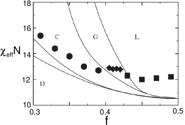
Figure 3.8: Phase diagrams for diblock copolymer melts as obtained from Monte Carlo simulations of a lattice model (chain length $N=30$) by Matsen et al. (left) [338] and from field-theoretical Complex-Langevin simulations (Ginzburg parameter $C=50$) by Lennon et al (right) [342]. Symbols L,C,G correspond to diblock phases of Fig. 3.3; in addition, the Monte Carlo phase diagram features a perforated lamellar (PL) phase. Left figure: Courtesy of Mark W. Matsen, adapted from Matsen, Griffiths, Wickham, and Vassiliev, J. Chem. Phys. 124, 024904 (2006). Right figure: Reprinted with permission from Lennon, Katsov, , and Fredrickson, Phys. Rev. Lett. 101, 138302, 2008. Copyright (2008) by the American Physical Society.

Two examples of phase diagrams obtained with different simulation methods are shown in Fig. 3.8: One was calculated by Matsen et al [338] using Monte Carlo simulations of copolymers with length $N=30$ in a simple lattice model (left), and one by Lennon et al.[342] using field-theoretical calculations (right) at Ginzburg parameter $C=50$. Both phase diagrams significantly improve on the SCF phase diagram of Fig. 3.5 (right) in the weak segregation regime, and reproduce the main qualitative features of the experimental phase diagram (Fig. 3.5, left): The transitions are first order everywhere. The ODT is shifted to higher $\chi N$. Direct phase transition between the disordered phase and the complex mesophase (PL or G, respectively) or the lamellar phase are possible for a range of copolymer block fractions $f$. The phase diagrams even reproduce a small hump of the ODT transition line at the boundary to the complex mesophase (PL or G), which is also observed experimentally. The only ’problem’ with the Monte Carlo phase diagram is that it features a perforated lamellar (PL) phase instead of a gyroid (G) phase. This may be a finite size artefact, as suggested by the authors, or a property of the lattice model under consideration. (Gyroid phases have been found in lattice models [204], but it should be noted that the free energies of the PL and the G phase are very close according to SCF calculations.) Nevertheless, the simulations demonstrate convincingly that the discrepancies between the experimental phase diagram and the SCF phase diagram shown in Fig. 3.5 can to a large extent be attributed to the effect of fluctuations.

In recent years, researchers have also begun to simulate melts of more complex copolymers, e.g., starblock copolymers [343, 344, 345, 346, 347], rod-coil copolymers, [348, 349] diblock copolymers with one crystallizing component [25, 24, 350, 26, 351, 352], triblock copolymers [353, 354, 355, 356], or random copolymers [357, 358]. An interesting study on diblock copolymers with one amphiphilic block has recently been presented by Khokholov and Khalatur [359]. Since the amphiphilic block favors interfaces, the morphology of the mesophases changes completely and is characterized by thin channels and slits. Lay et al. and Palmer et al have studied the computationally challenging problem of microphase separation in randomly crosslinked binary blends [360, 361, 362], and also the inverse problem, to which extent ordered copolymer structures can be stabilized by cross-linking [363].

A large amount of simulation work on copolymer melts has been done with time-dependent Ginzburg-Landau approaches [364, 365, 366, 367, 368, 369, 370, 371, 372, 373, 374, 375, 376, 377, 378]. These studies have mostly addressed dynamical questions, i.e., the kinetics of ordering, disordering processes in pure melts [366, 367, 368, 369, 370, 371, 372, 373, 374] and in mixtures containing copolymers [375, 376, 377, 378]. Already in pure diblock copolymer melts, ordering/disordering processes were found to proceed via intricate pathways that involve nontrivial intermediate states (e.g., the perforated lamellar state which is only metastable at equilibrium). In mixtures, the interplay of macrophase and microphase separation leads to a wealth of new transient morphologies [375, 376, 377, 378] (see also Ref. 379).

Confined Copolymer Melts

In recent years, there has been growing interest in confined copolymer systems. The first studies have explored the ordering of copolymers melts in thin films between neutral walls [380, 381, 382, 383] or general (selective) walls [384, 385, 386, 387, 388, 389, 390, 391, 392, 393, 394], both with particle-based models and dynamic density field theories. Triblock copolymers [395, 396, 397, 398, 399, 400] and copolymer blends [382] have also been considered. The dynamics of copolymer ordering in confinement was studied with time-dependent Ginzburg-Landau methods [401, 402, 392]. A series of papers have dealt with the technologically relevant question, whether and how surface patterns can be transferred into copolymer films, [403, 404, 389, 405, 406, 407, 408].

The current focus shifts to nanocylindrically or spherically confined blends [409, 410, 411, 412, 205, 413, 414, 415, 416, 417, 418]. A variety of new structures can already be observed in systems of diblock copolymers confined to nanocylinders, e.g., mesh structures, single and double helices [410]. For triblock copolymers, the spectrum is even more diverse [205]. The confined structures depend on the bulk structure and on the shape of the confining channels. Li and coworkers have shown that possible morphologies can be screened efficiently with the method of simulated annealing [419, 420, 421, 422, 423, 424].

Copolymers under Shear

Finally in this section, I briefly mention the large amount of work that has addressed the effect of shear on the microstructure of copolymer systems, with both field-based and particle-based methods [425, 426, 427, 428, 429, 430, 431, 432, 433, 434, 435, 436, 437, 438, 439, 440, 441]. Special attention was given to the phenomenon that lamellae reorient under shear [431, 442, 443, 444, 445]. Experimentally, it is observed that lamellae orient parallel to the shear flow at low shear rates, and perpendicular to the shear flow at high shear rates. Simulations give conflicting results. The parallel state consistently becomes unstable at high shear rates, but its relative stability at low shear rates (or results on the indicators of relative stability such as the entropy production) seems to depend on the type of model [443, 445].

V Future Challenges

The equilibrium theory of fluid polymer mixtures is fairly advanced. Thanks to the universal properties of polymers, it requires relatively little input information ($\chi$ parameter etc.) to be predictive at a quantitative level. However, if one goes beyond equilibrium and beyond the fluid state, the situation is much less satisfying. For example, very little work has been done on crosslinked polymer blends [363, 360, 361, 362], even though they are common in applications. Physical crosslinks can be established if domains crystallize or become glassy. As we have seen above, research on blends with one crystallizing or glassy component is also rather scarce.

Another important issue is the influence of the blend processing on the properties of the resulting materials, i.e., the structure of phase separating blends under shear. The mechanical properties of immiscible blends depend crucially on their microscopic morphologies, i.e., the sizes and shapes of droplets, which in turn depend on the manufacturing process. Theoretical nonequilibrium state diagrams that relate the processing conditions (shear rates, geometry, copolymer concentration etc.) with final morphologies are still missing. Since the relevant length scales are relatively large and hydrodynamics are important, the simulation method of choice should be a cell dynamics method that incorporates hydrodynamics, e.g., a Lattice-Boltzmann method [446]. Methods that combine Ginzburg-Landau functionals for immiscible fluids with Lattice-Boltzmann models for Newtonian fluids have been developed [447] and used to study demixing processes at rest [448] and under shear [449, 450, 451]. Giraud and coworkers have proposed a Lattice-Boltzmann method for viscoelastic fluids, which is more suitable to describe polymers [452], and carried out first simulations of viscoelastic liquid mixtures [453]. Nevertheless, the whole field is still in its infancy.

As the field of polymer simulations reaches maturity, the bottom-up modeling approach (Sec. IV.1) will gain importance. So far, the vast majority of theoretical and simulation studies of (co)polymer blends was based on generic model systems. One or two decades from now, realistic simulations of specific polymer blends will probably be equally, if not more common. One of the major challenges in this context is to develop hybrid multiscale methods that combine different levels of coarse-graining, i.e., use a relatively coarse basic model and fine-grain selectively in interesting regions of the materials (e.g., interfaces) [166].

Acknowledgments

The author thanks Mark W. Matsen for introducing her to the self-consistent field theory a long time ago and for providing Figs. 3.5 and 3.8 (left), and Glenn H. Fredrickson for discussions and for the permission to show Fig. 3.8 (right). She has benefitted from collaborations and/or discussions with Jörg Baschnagel, Kurt Binder, Dominik Düchs, Burkhard Dünweg, Avi Halperin, Venkat Ganesan, Kurt Kremer, Marcus Müller, Wolfgang Paul, Ulf Schiller, Jens Smiatek, Jens-Uwe Sommer, Andreas Werner, and many others. Financial support from the German Science Foundation (DFG) is gratefully acknowledged.

Bibliography

- [1] Flory P. J. Chem. Phys. 1941; 9:660–661.
- [2] Huggins M. J. Chem. Phys. 1941; 9:440.
- [3] Flory P. Statistical mechanics of chain molecules. edn., John Wiley & Sons: New York, 1969.
- [4] de Gennes P. Scaling concepts in polymer physics. edn., Cornell University Press: Cornell, 1979.
- [5] Doi M, Edwards S. The theory of polymer dynamics. edn., Oxford University Press: New York, 1986.
- [6] Fleer G, Cohen Stuart M, Scheutjens J, Cosgrove T, Vincent B. Polymers at interfaces. edn., Kluwer Academic Publ: Reading, Massachusetts, 1993.
- [7] Larson R. The structure and rheology of complex fluids. edn., Oxford University Press: New York, 1999.
- [8] Fredrickson G. The equilibrium theory of inhomogeneous polymers. edn., Clarendon press: Oxford, 2006.
- [9] Hamley I. The physics of block copolymers. edn., Oxford University Press: Oxford, 1999.
- [10] Guth E, Mark H. Monatshefte für Chemie 1934; 65:93.
- [11] Paul W, J B. Stochastic processes from physics to finance. edn., Springer: Berlin, 1999.
- [12] Kleinert H. Path integrals in quantum mechanics, polymer physics, and financial markets. 5th edn., World Scientific: , 2009.
- [13] Osa M, Yoshizaki T, Yamakawa H. Polymer JOURNAL 2004; 36:634–641.
- [14] Duplantier B, Saleur H. Nucl. Phys. B 1987; 290:291–326.
- [15] Semenov A, Johner A. Eur. Phys. J. E 2003; 12:469–480.
- [16] Zhulina EB, Borisov OV. Macromolecules 2008; 41:5934–5944.
- [17] Daoud M, Cotton J, Farnoux B, Jannink G, Sarma G, Benoit H, Duplessis R, Picot C, de Gennes P. Macromolecules 1975; 8:804–818.
- [18] Cacciuto A, Luijten E. Nano Lett. 2006; 6:901–905.
- [19] Wittmer J, Meyer H, Baschnagel J, Johner A, Obukhov S, Mattioni L, Muller M, Semenov A. Phys. Rev. Lett. 2004; 93:147 801.
- [20] Wittmer JP, Beckrich P, Johner A, Semenov AN, Obukhov SP, Meyer H, Baschnagel J. EPL 2007; 77:56 003.
- [21] Ahlrichs P, Everaers R, Dünweg B. Phys. Rev. E 2001; 64:040 501.
- [22] McLeish T. Adv. Phys. 2002; 51:1379–1527.
- [23] Hu W, Mathot V. J. Chem. Phys. 2003; 119:10 953–10 957.
- [24] Hu W. Macromolecules 2005; 38:3977–3983.
- [25] Hu W, Frenkel D. Faraday. Disc. 2005; 128:253–260.
- [26] Wang M, Hu W, Ma Y, Ma Y. J. Chem. Phys. 2006; 124:244 901.
- [27] Ma Y, Hu W, Wang H. Phys. Rev. E 2007; 76:031 801.
- [28] Ma Y, Zha L, Hu W, Reiter G, Han CC. Phys. Rev. E 2008; 77:061 801.
- [29] Mehta R, Kyu T. J. Pol. Sci. B 2004; 42:2892–2899.
- [30] Zhou D, Shi AC, Zhang P. J. Chem. Phys. 2008; 129:154 901.
- [31] Khalatur P, Khokholov A, Vasilevskaya V. Macrom. Theory and Sim. 1994; 3:939–961.
- [32] Genix A, Arbe A, Alvarez F, Colmenero J, Willner L, Richter D. Phys. Rev. E 2005; 72:031 808.
- [33] Han C, Bauer B, Clark J, Muroga Y, Matsushita Y, Okada M, Qui T, Chang T, Sanchez I. Polymer 1988; 29:2002–2014.
- [34] Hildebrand J, Scott R. The solubility of non-electrolytes. edn., Dover: New York, 1964.
- [35] Biros J, Zeman L, Patterson D. Macromolecules 1971; 4:30–&.
- [36] Freed K, Dudowicz J. Trends in Polymer Science 1995; 3:248–255.
- [37] Foreman K, Freed K. Adv. Chem. Phys. 1998; 103:335–390.
- [38] Dudowicz J, Freed K, Douglas J. Phys. Rev. Lett. 2002; 88:095 503.
- [39] Dudowicz J, Freed K, Douglas J. J. Chem. Phys. 2002; 116:9983–9996.
- [40] Freed K, Dudowicz J. Adv. Pol. Science 2005; 183:63–126.
- [41] Kumar S. Macromolecules 2000; 33:5285–5291.
- [42] Taylor J, Debenedetti P, Graessley W, Kumar S. Macromolecules 1996; 29:764–773.
- [43] Melenkevitz J, Crist B, Kumar S. Macromolecules 2000; 33:6869–6877.
- [44] Müller M, Binder K. Macromolecules 1995; 28:1825–1834.
- [45] Müller M, Binder K. J. Physique II 1996; 6:187–194.
- [46] Fried H, Binder K. J. Chem. Phys. 1991; 94:8349–8366.
- [47] Fried H, Binder K. Europhys. Lett. 1991; 16:237–242.
- [48] Maurer W, Bates F, Lodge T, Almdal K, Mortensen K, Fredrickson G. J. Chem. Phys. 1998; 108:2989–3000.
- [49] Freed K, Dudowicz J. Macromolecules 1998; 31:6681–6690.
- [50] Dudowicz J, Freed K. Macromolecules 2000; 33:3467–3477.
- [51] Curro J, Schweizer K. J. Chem. Phys. 1988; 88:7242–7243.
- [52] Schweizer K. Macromolecules 1993; 26:6033–6049.
- [53] Schweizer K, Curro J. Adv. Chem. Phys. 1997; 98:1–142.
- [54] Wang Z. J. Chem. Phys. 2002; 117:481–500.
- [55] Akkermans RLC. J. Chem. Phys. 2008; 128:244 904.
- [56] Tambasco M, Lipson J, Higgins J. Macromolecules 2006; 39:4860–4868.
- [57] Lipson J. Macromolecules 1991; 24:1334–1340.
- [58] Lipson J, Andrews S. J. Chem. Phys. 1992; 96:1426–1434.
- [59] Tambasco M, Lipson J, Higgins J. Macromolecules 2004; 37:9219–9230.
- [60] Freed K, Pesci A. J. Chem. Phys. 1987; 87:7342–7344.
- [61] Shibayama M, Yang H, Stein R, Han C. Macromolecules 1985; 18:2179–2187.
- [62] Balsara N, Fetters L, Hadjichristidis N, Lohse D, Han C, Graessely W, Krishnamoorti R. Macromolecules 1992; 25:6137–6147.
- [63] Londono J, Wignall G. Macromolecules 1997; 30:3821–3824.
- [64] Fan C, Olafson B, Blanco M, Hsu S. Macromolecules 1992; 25:3667–3676.
- [65] Kipper M, Seifert S, Thiyagarajan P, Narasimhan B. Polymer 2004; 45:3329–3340.
- [66] Helfand E, Tagami Y. J. Pol. Sci. B Lett. 1971; 9:741–&.
- [67] Helfand E, Tagami Y. J. Chem. Phys. 1972; 57:1812–&.
- [68] Helfand E, Tagami Y. J. Chem. Phys. 1972; 56:3592–&.
- [69] Helfand E, Sapse A. J. Chem. Phys. 1975; 62:1327–1331.
- [70] Helfand E. J. Chem. Phys. 1975; 62:999–1005.
- [71] Schmid F. J. Phys.: Cond. Matt. 1998; 10:8105–8138.
- [72] Matsen M. J. Phys.: Cond. Matt. 2002; 14:R21–R47.
- [73] Freed K. J. Chem. Phys. 1995; 103:3230–3239.
- [74] Hong K, Noolandi J. Macromolecules 1981; 14:727–736.
- [75] Schmid F. J. Chem. Phys. 1996; 104:9191–9201.
- [76] Matsen M, Schick M. Macromolecules 1994; 27:6761–6767.
- [77] Morse D, Fredrickson G. Phys. Rev. Lett. 1994; 73:3235–3238.
- [78] Duchs D, Sullivan D. J. Phys.: Cond. Matt. 2002; 14:12 189–12 202.
- [79] Hidalgo RC, Sullivan DE, Chen JZY. J. Phys.: Cond. Matt. 2007; 19:376 107.
- [80] Wang Q, Taniguchi T, Fredrickson G. J. Phys. Chem. B 2004; 108:6733–6744.
- [81] Cooke DM, Shi AC. Macromolecules 2006; 39:6661–6671.
- [82] Lynd NA, Hillmyer MA, Matsen MW. Macromolecules 2008; 41:4531–4533.
- [83] Hall DM, Lookman T, Fredrickson GH, Banerjee S. Phys. Rev. Lett. 2006; 97:114 501.
- [84] Maniadis P, Lookman T, Kober EM, Rasmussen KO. Phys. Rev. Lett. 2007; 99:048 302.
- [85] Feng EH, Lee WB, Fredrickson GH. Macromolecules 2007; 40:693–702.
- [86] Lee WB, Elliott R, Katsov K, Fredrickson GH. Macromolecules 2007; 40:8445–8454.
- [87] Thompson R, Ginzburg V, Matsen M, Balazs A. Science 2001; 292:2469–2472.
- [88] Reister E, Fredrickson G. J. Chem. Phys. 2005; 123:214 903.
- [89] Sides S, Kim B, Kramer E, Fredrickson G. Phys. Rev. Lett. 2006; 96:250 601.
- [90] Zinn-Justin J. Quantum field theory and critical phenomena. 2nd edn., Clarendon Press: Oxford, 1993.
- [91] Müller M, Schmid F. Adv. Pol. Science 2005; 185:1–58.
- [92] Matsen M, Schick M. Phys. Rev. Lett. 1994; 72:2660–2663.
- [93] Matsen M, Bates F. Macromolecules 1996; 29:1091–1098.
- [94] Bates F, Schulz M, Khandpur A, Forster S, Rosedale J, Almdal K, Mortensen K. Faraday. Disc. 1994; 98:7–18.
- [95] Förster S, Khandpur A, Zhao J, Bates F, Hamley I, Ryan A, Bras W. Macromolecules 1994; 27:6922–6935.
- [96] Khandpur A, Förster S, Bates F, Hamley I, Ryan A, Bras W, Almdal K, Mortensen K. Macromolecules 1995; 28:8796–8806.
- [97] Tyler C, Morse D. Phys. Rev. Lett. 2005; 94:208 302.
- [98] Takenaka M, Wakada T, Akasaka S, Nishitsuji S, Saijo K, Shimizu H, Kim MI, Hasegawa H. Macromolecules 2007; 40:4399–4402.
- [99] Scheutjens J, Fleer G. J. Phys. Chem. 1979; 83:1619–1635.
- [100] Carignano M, Szleifer I. J. Chem. Phys. 1993; 98:5006–5018.
- [101] Bryk P, MacDowell LG. J. Chem. Phys. 2008; 129:104 901.
- [102] Tang H, Freed K. J. Chem. Phys. 1991; 94:1572–1583, doi:10.1063/1.459962.
- [103] Woodward C. J. Chem. Phys. 1991; 94:3183–3191.
- [104] Woodward C, Yethiraj A. J. Chem. Phys. 1994; 100:3181–3186.
- [105] Fraaije J. J. Chem. Phys. 1993; 99:9202–9212.
- [106] Fraaije J, vanVlimmeren B, Maurits N, Postma M, Evers O, Hoffmann C, Altevogt P, GoldbeckWood G. J. Chem. Phys. 1997; 106:4260–4269.
- [107] Hasegawa R, Doi M. Macromolecules 1997; 30:3086–3089.
- [108] Kawakatsu T. Phys. Rev. E 1997; 56:3240–3250.
- [109] Hillmyer M, Maurer W, Lodge T, Bates F, Almdal K. J. Phys. Chem. B 1999; 103:4814–4824.
- [110] Düchs D, Ganesan V, Fredrickson G, Schmid F. Macromolecules 2003; 36:9237–9248.
- [111] Düchs D, Schmid F. J. Chem. Phys. 2004; 121:2798–2805.
- [112] Herktmätzki C, Schelten J. Phys. Rev. Lett. 1983; 51:896–899.
- [113] Schwahn D, Mortensen K, Yeemadeira H. Phys. Rev. Lett. 1987; 58:1544–1546.
- [114] Holyst R, Vilgis T. J. Chem. Phys. 1993; 99:4835–4844.
- [115] Brazovskii S. Sov. Phys. JETP 1975; 41:85.
- [116] Fredrickson G, Helfand E. J. Chem. Phys. 1987; 87:697–705.
- [117] Shi A, Noolandi J, Desai R. Macromolecules 1996; 29:6487–6504.
- [118] Leibler L. Macromolecules 1980; 13:1602–1617.
- [119] Milner S, Olmsted P. J. Physique II 1997; 7:249–255.
- [120] Erukhimovich I. Eur. Phys. J. E 2005; 18:383–406.
- [121] Ohta T, Kawasaki K. Macromolecules 1986; 19:2621–2632.
- [122] Ohta T, Kawasaki K. Macromolecules 1990; 23:2413–2414.
- [123] Uneyama T, Doi M. Macromolecules 2005; 38:196–205.
- [124] Yamada K, Nonomura M, Ohta T. J. Phys.: Cond. Matt. 2006; 18:L421–L427.
- [125] Kawakatsu T. Phys. Rev. E 1994; 50:2856–2862.
- [126] Kielhorn L, Muthukumar M. J. Chem. Phys. 1999; 110:4079–4089.
- [127] Sakurai J. Modern Quantum Mechanics. edn., Addison-Wesley: , 1994.
- [128] Semenov A. Sov. Phys. JETP 1985; 61:733–742.
- [129] Milner S, Witten T, Cates M. Europhys. Lett. 1988; 5:413–418.
- [130] Zhulina E, Borisov O, Pryamitsyn V. J. Coll. Interf. Sci. 1990; 137:495–511.
- [131] Zhulina E, Borisov O, Pryamitsyn V, Birshtein T. Macromolecules 1991; 24:140–149.
- [132] Milner S, Witten T, Cates M. Macromolecules 1988; 21:2610–2619.
- [133] Witten T, Leibler L, Pincus P. Macromolecules 1990; 23:824–829.
- [134] Matsen M. J. Chem. Phys. 2001; 114:10 528–10 530.
- [135] Netz R, Schick M. Europhys. Lett. 1997; 38:37–42.
- [136] Netz R, Schick M. Macromolecules 1998; 31:5105–5122.
- [137] Carelli C, Jones R, Young R, Cubitt R, Dalgliesh R, Schmid F, Sferrazza M. Phys. Rev. E 2005; 72:031 807.
- [138] Fernandez M, Higgins J, Penfold J, Ward R, Shackleton C, Walsh D. Polymer 1988; 29:1923–1928.
- [139] Stamm M, Schubert D. Ann. Rev. Mat. Sci. 1995; 25:325–356.
- [140] Schubert D, Stamm M. Europhys. Lett. 1996; 35:419–424.
- [141] Kerle T, Klein J, Binder K. Phys. Rev. Lett. 1996; 77:1318–1321.
- [142] Sferrazza M, Xiao C, Jones R, Bucknall D, Webster J, Penfold J. Phys. Rev. Lett. 1997; 78:3693–3696.
- [143] Carelli C, Jones R, Young R, Cubitt R, Krastev R, Gutberlet T, Dalgliesh R, Schmid F, Sferrazza M. Europhys. Lett. 2005; 71:763–769.
- [144] Buff F, Lovett R, Stillinger F. Phys. Rev. Lett. 1965; 15:621–&.
- [145] Rowlinson J, Widom B. Molecular Theory of Capillarity. edn., Clarendon: Oxford, 1982.
- [146] Semenov A. Macromolecules 1994; 27:2732–2735.
- [147] Lacasse M, Grest G, Levine A. Phys. Rev. Lett. 1998; 80:309–312.
- [148] Werner A, Schmid F, Müller M, Binder K. Phys. Rev. E 1999; 59:728–738.
- [149] Schmid F, Müller M. Macromolecules 1995; 28:8639–8645.
- [150] Forster D. Hydrodynamic fluctuations, broken symmetry, and correlation functions. edn., Addison-Wesley: Reading, Massachusetts, 1995.
- [151] Baschnagel J, Binder K, Doruker P, Gusev A, Hahn O, Kremer K, Mattice W, Müller-Plathe F, Murat M, Paul W, et al.. Adv. Pol. Science 2000; 152:41–156.
- [152] Müller-Plathe F. ChemPhysChem 2002; 3:754–769.
- [153] Müller-Plathe F. Soft Materials 2003; 1:1–31.
- [154] Binder K, Paul W, Sanots S, UW S. 2004; 152:491–510.
- [155] Baschnagel J, Binder K, Paul W, Laso M, Suter U, Batoulis I, Jilge W, Burger T. J. Chem. Phys. 1991; 95:6014–6025.
- [156] Paul W, Pistoor N. Macromolecules 1994; 27:1249–1255.
- [157] Rapold R, Mattice W. J. Chem. Soc. - Far. Transactions 1995; 91:2435–2441.
- [158] Carbone P, Varzaneh HAK, Chen X, Mueller-Plathe F. J. Chem. Phys. 2008; 128:064 904.
- [159] Reith D, Pütz M, Müller-Plathe F. J. Comp. Chem. 2003; 24:1624–1636.
- [160] Faller R. Polymer 2004; 45:3869–3876.
- [161] Milano G, Müller-Plathe F. J. Phys. Chem. B 2005; 109:18 609–18 619.
- [162] Li X, Kou D, Rao S, Liang H. J. Chem. Phys. 2006; 124:204 909.
- [163] Santangelo G, Di Matteo A, Muller-Plathe F, Milano G. J. Phys. Chem. B 2007; 111:2765–2773.
- [164] Sewell TD, Rasmussen KO, Bedrov D, Smith GD, Thompson RB. J. Chem. Phys. 2007; 127:144 901.
- [165] Guenza MG. J. Phys.: Cond. Matt. 2008; 20:033 101.
- [166] Praprotnik M, Delle Site L, Kremer K. Ann. Rev. Phys. Chem. 2008; 59:545–571.
- [167] Honda T, Kawakatsu T. Macromolecules 2007; 40:1227–1237.
- [168] Akten E, Mattice W. Macromolecules 2001; 34:3389–3395.
- [169] Rane S, Mattice W, Dhinojwala A. J. Phys. Chem. B 2004; 108:14 830–14 839.
- [170] Choi P, Rane SS, Mattice WL. Macrom. Theory and Sim. 2006; 15:563–572.
- [171] Sun Q, Faller R. J. Chem. Theory and Comp. 2006; 2:607–615.
- [172] Sun Q, Faller R. J. Chem. Phys. 2007; 126:144 908.
- [173] Sun Q, Pon FR, Faller R. Fluid Phase Equilibria 2007; 261:35–40.
- [174] Choi K, Jo W. Macromolecules 1997; 30:1509–1514.
- [175] Lee S, Lee J, Lee H, Mumby S. Polymer 1999; 40:5137–5145.
- [176] Gestoso P, Brisson J. Polymer 2003; 44:2321–2329.
- [177] Gestoso P, Brisson J. Polymer 2003; 44:7765–7776.
- [178] Maranas J, Kumar S, Debenedetti P, Graessley W, Mondello M, Grest G. Macromolecules 1998; 31:6998–7002.
- [179] Maranas J, Mondello M, Grest G, Kumar S, Debenedetti P, Graessley W. Macromolecules 1998; 31:6991–6997.
- [180] Neelakantan A, Maranas J. Macromolecules 2004; 37:8473–8480.
- [181] Faller R. Macromolecules 2004; 37:1095–1101.
- [182] Rissanou AN, Peristeras LD, Economou IG. Polymer 2007; 48:3883–3892.
- [183] Prathab B, Subramanian V, Aminabhavi TM. Polymer 2007; 48:417–424.
- [184] Prathab B, Aminabhavi TM. Langmuir 2007; 23:5439–5444.
- [185] Tao H, Fan C, Macknight W, Hsu S. Macromolecules 1994; 27:1720–1728.
- [186] Spyriouni T, Vergelati C. Macromolecules 2001; 34:5306–5316.
- [187] Yang H, Li Z, Lu Z, Sun C. Eur. Pol. J. 2005; 41:2956–2962.
- [188] Jawalkar S, Adoor S, Sairam M, Nadagouda M, Aminabhavi T. J. Phys. Chem. B 2005; 109:15 611–15 620.
- [189] Jawalkar SS, Aminabhavi TM. Polymer 2006; 47:8061–8071.
- [190] Jawalkar SS, Raju KVSN, Halligudi SB, Sairam M, Aminabhavi TM. J. Phys. Chem. B 2007; 111:2431–2439.
- [191] Jawalkar SS, Nataraj SK, Raghu AV, Aminabhavi TM. J. Appl. Pol. Sci. 2008; 108:3572–3576.
- [192] Lee WJ, Ju SP, Wang YC, Chang JG. J. Chem. Phys. 2007; 127:064 902.
- [193] Lu Z, Li Z, Huang X, Jiang B, Sun J. Macrom. Theory and Sim. 1998; 7:619–622.
- [194] Pavel D, Shanks R. Polymer 2005; 46:6135–6147.
- [195] Sariban A, Binder K, Heermann D. Coll. Pol. Sci. 1987; 265:424–431.
- [196] Sariban A, Binder K. Macromolecules 1988; 21:711–726.
- [197] Cifra P, Karasz F, Macknight W. J. Pol. Sci. B 1988; 26:2379–2383.
- [198] Frenkel D, Smit B. Understanding molecular simulation. 2nd edn., Academic Press: San Diego, 2002.
- [199] Ferrario M, Ciccotti G, Binder K ( (eds.)). Computer simulations in condensed matter: From materials to chemical biology, vol. 2. Springer: Berlin, 2006.
- [200] Larson R, Scriven L, Davis H. J. Chem. Phys. 1985; 83:2411–2420.
- [201] Dotera T, Hatano A. J. Chem. Phys. 1996; 105:8413–8427.
- [202] Pakula T. Macromolecules 1987; 20:679–682.
- [203] Carmesin I, Kremer K. Macromolecules 1988; 21:2819–2823.
- [204] Martinez-Veracoechea F, Escobedo F. Macromolecules 2005; 38:8522–8531.
- [205] Feng J, Ruckenstein E. J. Chem. Phys. 2007; 126:124 902.
- [206] Grest G, Lacasse M, Kremer K, Gupta A. J. Chem. Phys. 1996; 105:10 583–10 594.
- [207] Groot R, Warren P. J. Chem. Phys. 1997; 107:4423–4435.
- [208] Klapp S, Diestler D, Schoen M. J. Phys.: Cond. Matt. 2004; 16:7331–7352.
- [209] Laradji M, Guo H, Zuckermann M. Phys. Rev. E 1994; 49:3199–3206.
- [210] Soga K, Zuckermann M, Guo H. Macromolecules 1996; 29:1998–2005.
- [211] Besold G, Hassager O, Mouritsen O. Comp. Phys. Comm. 1999; 121:542–544.
- [212] Besold G, Guo H, Zuckermann M. J. Pol. Sci. B 2000; 38:1053–1068.
- [213] Detcheverry FA, Kang H, Daoulas KC, Mueller M, Nealey PF, de Pablo JJ. Macromolecules 2008; 41:4989–5001.
- [214] Müller M, Wittmer J, Cates M. Phys. Rev. E 1996; 53:5063–5074.
- [215] Müller M, Daoulas KC. J. Chem. Phys. 2008; 129:164 906.
- [216] Murat M, Kremer K. J. Chem. Phys. 1998; 108:4340–4348.
- [217] Eurich F, Maass P. J. Chem. Phys. 2001; 114:7655–7668.
- [218] Eurich F, Maass P, Baschnagel J. J. Chem. Phys. 2002; 117:4564–4577.
- [219] Eurich F, Karatchentsev A, Baschnagel J, Dieterich W, Maass P. J. Chem. Phys. 2007; 127:134 905.
- [220] Sambriski EJ, Guenza MG. Phys. Rev. E 2007; 76:051 801.
- [221] Fredrickson G, Ganesan V, Drolet F. Macromolecules 2002; 35:16–39.
- [222] Fredrickson GH. Soft Matter 2007; 3:1329–1334.
- [223] Lennon EM, Mohler GO, Ceniceros HD, Garcia-Cervera CJ, Fredrickson GH. Multiscale Modeling and Simulation 2007; 6:1347–1370.
- [224] Ganesan V, Fredrickson G. Europhys. Lett. 2001; 55:814–820.
- [225] Barrat J, Fredrickson G, Sides S. J. Phys. Chem. B 2005; 109:6694–6700.
- [226] Popov YO, Lee J, Fredrickson GH. J. Pol. Sci. B 2007; 45:3223–3230.
- [227] Lee J, Popov YO, Fredrickson GH. J. Chem. Phys. 2008; 128:224 908.
- [228] Moreira A, Bäurle S, Fredrickson G. Phys. Rev. Lett. 2003; 91:150 201.
- [229] Bäurle SA, Efimov GV, Nogovitsin EA. Europhys. Lett. 2006; 75:378–384.
- [230] Bäurle S, Efimov G, Nogovitsin E. J. Chem. Phys. 2006; 124:224 110.
- [231] Risken H. The Fokker-Planck equation. 2nd edn., Springer: Berlin, 1989.
- [232] Hoogerbrugge P, Koelman J. Europhys. Lett. 1992; 19:155–160.
- [233] Espanol P, Warren P. Europhys. Lett. 1995; 30:191–196.
- [234] Soddemann T, Dünweg B, Kremer K. Phys. Rev. E 2003; 68:046 702.
- [235] Groot R, Madden T, Tildesley D. J. Chem. Phys. 1999; 110:9739–9749.
- [236] Müller M, Smith G. J. Pol. Sci. B 2005; 43:934–958.
- [237] Daoulas KC, Müller M. J. Chem. Phys. 2006; 125:184 904.
- [238] Ganesan V, Pryamitsyn V. J. Chem. Phys. 2003; 118:4345–4348.
- [239] Baeurle SA, Usami T, Gusev AA. Polymer 2006; 47:8604–8617.
- [240] Maurits N, vanVlimmeren B, Fraaije J. Phys. Rev. E 1997; 56:816–825.
- [241] Maurits N, Fraaije J. J. Chem. Phys. 1997; 107:5879–5889.
- [242] Reister E, Müller M, Binder K. Phys. Rev. E 2001; 64:041 804.
- [243] He X, Schmid F. Macromolecules 2006; 39:2654–2662.
- [244] He X, Schmid F. Macromolecules 2006; 39:8908–8910.
- [245] He X, Schmid F. Phys. Rev. Lett. 2008; 100:137 802.
- [246] Maurits N, Zvelindovsky A, Fraaije J. J. Chem. Phys. 1998; 109:11 032–11 042.
- [247] Maurits N, Zvelindovsky A, Sevink G, van Vlimmeren B, Fraaije J. J. Chem. Phys. 1998; 108:9150–9154.
- [248] Honda T, Kawakatsu T. J. Chem. Phys. 2008; 129:114 904.
- [249] Mihajlovic M, Lo T, Shnidman Y. Phys. Rev. E 2005; 72:041 801.
- [250] Oono Y, Shiwa Y. Mod. Phys. Lett. B 1987; 1:49–55.
- [251] Bahiana M, Oono Y. Phys. Rev. A 1990; 41:6763–6771.
- [252] Deutsch H, Binder K. Macromolecules 1992; 25:6214–6230.
- [253] Deutsch H, Binder K. J. Physique II 1993; 3:1049–1073.
- [254] Binder K. Adv. Pol. Science 1994; 112:181–299.
- [255] Müller M, Wilding N. Phys. Rev. E 1995; 51:2079–2089.
- [256] Dadmun M, Waldow D. Phys. Rev. E 1999; 60:4545–4550.
- [257] Forrest B, Toral R. J. Stat. Phys. 1994; 77:473–489.
- [258] Sariban A, Binder K. Macromolecules 1991; 24:578–592.
- [259] Brown G, Chakrabarti A. Phys. Rev. E 1993; 48:3705–3711.
- [260] Takenaka M, Hashimoto T, Dobashi T. Phys. Rev. E 1995; 52:5142–5145.
- [261] Cao Y, Zhang H, Xiong Z, Yang Y. Macrom. Theory and Sim. 2001; 10:314–324.
- [262] Cheng M, Nauman E. J. Pol. Sci. B 2004; 42:603–612.
- [263] Prusty M, Keestra BJ, Goossens JGP, Anderson PD. Chem. Eng. Science 2007; 62:1825–1837.
- [264] He D, Nauman E. Chem. Eng. Science 1997; 52:481–496.
- [265] Zhang Z, Zhang H, Yang Y, Vinckier I, Laun H. Macromolecules 2001; 34:1416–1429.
- [266] Xu H, Chiu HW, Okabe Y, Kyu T. Phys. Rev. E 2006; 74:011 801.
- [267] Müller M. Macrom. Theory and Sim. 1999; 8:343–374.
- [268] Kumar S. Macromolecules 1994; 27:260–271.
- [269] Yang Y, Lu J, Yan D, Ding J. Macrom. Theory and Sim. 1994; 3:731–741.
- [270] Müller M. Macromolecules 1995; 28:6556–6564.
- [271] Weinhold J, Kumar S, Singh C, Schweizer K. J. Chem. Phys. 1995; 103:9460–9474.
- [272] Theodorakis PE, Avgeropoulos A, Freire JJ, Kosmas M, Vlahos C. J. Phys.: Cond. Matt. 2007; 19:466 111.
- [273] Reiter J, Zifferer G, Olaj O. Macromolecules 1990; 23:224–228.
- [274] Müller M, Binder K, Oed W. J. Chem. Soc. - Far. Transactions 1995; 91:2369–2379.
- [275] Ypma G, Cifra P, Nies E, vanBergen A. Macromolecules 1996; 29:1252–1259.
- [276] Olaj O, Petrik T, Zifferer G. J. Chem. Phys. 1998; 109:4646–4650.
- [277] Qian H, Lu Z, Chen L, Li Z, Sun C. J. Chem. Phys. 2005; 122:184 907.
- [278] Müller M, Werner A. J. Chem. Phys. 1997; 107:10 764–10 776.
- [279] Adhikari N, Auhl R, Straube E. Macrom. Theory and Sim. 2002; 11:315–325.
- [280] Adhikari N, Straube E. Macrom. Theory and Sim. 2003; 12:499–507.
- [281] Werner A, Schmid F, Müller M, Binder K. J. Chem. Phys. 1997; 107:8175–8188.
- [282] Werner A, Müller M, Schmid F, Binder K. J. Chem. Phys. 1999; 110:1221–1229.
- [283] Binder K, Müller M, Schmid F, Werner A. J. Stat. Phys. 1999; 95:1045–1068.
- [284] Barsky S, Robbins M. Phys. Rev. E 2001; 63:021 801.
- [285] Barsky S, Robbins M. Phys. Rev. E 2002; 65:021 808.
- [286] Narayanan B, Pryamitsyn V, Ganesan V. Macromolecules 2004; 37:10 180–10 194.
- [287] Lo T, Mihajlovic M, Shnidman Y, Li W, Gersappe D. Phys. Rev. E 2005; 72:040 801.
- [288] Kumar S, Tang H, Szleifer I. Mol. Phys. 1994; 81:867–872.
- [289] Rouault Y, Baschnagel J, Binder K. J. Stat. Phys. 1995; 80:1009–1031.
- [290] Rouault Y, Dunweg B, Baschnagel J, Binder K. Polymer 1996; 37:297–304.
- [291] Cifra P, Karasz F, Macknight W. Macromolecules 1992; 25:4895–4901.
- [292] Yethiraj A, Kumar S, Hariharan A, Schweizer K. J. Chem. Phys. 1994; 100:4691–4694.
- [293] Kumar S, Yethiraj A, Schweizer K, Leermakers F. J. Chem. Phys. 1995; 103:10 332–10 346.
- [294] Batman R, Gujrati PD. J. Chem. Phys. 2008; 128:124 903.
- [295] Cavallo A, Müller M, Binder K. Europhys. Lett. 2003; 61:214–220.
- [296] Cavallo A, Müller M, Binder K. J. Phys. Chem. B 2005; 109:6544–6552.
- [297] Pereira G, Wang J. J. Chem. Phys. 1996; 104:5294–5303.
- [298] Müller M, Binder K. Macromolecules 1998; 31:8323–8346.
- [299] Müller M, Binder K. Phys. Rev. E 2001; 63:021 602.
- [300] Morita H, Kawakatsu T, Doi M. Macromolecules 2001; 34:8777–8783.
- [301] Shang Y, Kazmer D, Wei M, Mead J, Barry C. J. Chem. Phys. 2008; 128:224 909.
- [302] Dadmun M. Macromolecules 1996; 29:3868–3874.
- [303] Dai B, Song M, Hourston D, He X, Liang H, Pan C. Polymer 2004; 45:1019–1026.
- [304] Werner A, Schmid F, Binder K, Müller M. Macromolecules 1996; 29:8241–8248.
- [305] Werner A, Schmid F, Müller M. J. Chem. Phys. 1999; 110:5370–5379.
- [306] Liang H. Macromolecules 1999; 32:8204–8209.
- [307] Kim S, Jo W. J. Chem. Phys. 1999; 110:12 193–12 201.
- [308] Milner S, Xi H. J. Rheol. 1996; 40:663–687.
- [309] Lyu S, Jones T, Bates F, Macosko C. Macromolecules 2002; 35:7845–7855.
- [310] Jo W, Kim S. Macromolecules 1996; 29:7204–7211.
- [311] Kim S, Jo W, Kim J. Macromolecules 1996; 29:6933–6940.
- [312] Kim S, Jo W, Kim J. Macromolecules 1997; 30:3910–3915.
- [313] Kim S, Jo W. J. Chem. Phys. 1998; 108:4267–4281.
- [314] Ko M, Kim S, Jo W. Polymer 2000; 41:6387–6394.
- [315] Müller M, Schick M. J. Chem. Phys. 1996; 105:8885–8901.
- [316] Poncela A, Rubio A, Freire J. J. Chem. Phys. 2003; 118:425–433.
- [317] Dotera T. Phys. Rev. Lett. 2002; 89:205 502.
- [318] Binder K, Fried H. Macromolecules 1993; 26:6878–6883.
- [319] Pakula T, Karatasos K, Anastasiadis S, Fytas G. Macromolecules 1997; 30:8463–8472.
- [320] Weyersberg A, Vilgis T. Phys. Rev. E 1993; 48:377–390.
- [321] Larson R. Macromolecules 1994; 27:4198–4203.
- [322] Larson R. Macromolecules 1995; 28:4784.
- [323] Pan X, Shaffer J. Macromolecules 1996; 29:4453–4455.
- [324] Hoffmann A, Sommer J, Blumen A. J. Chem. Phys. 1997; 106:6709–6721.
- [325] Banaszak M, Clarke J. Phys. Rev. E 1999; 60:5753–5756.
- [326] Jo W, Jang S. J. Chem. Phys. 1999; 111:1712–1720.
- [327] Murat M, Grest G, Kremer K. Europhys. Lett. 1998; 42:401–406.
- [328] Murat M, Grest G, Kremer K. Macromolecules 1999; 32:595–609.
- [329] Wang Q, Nealey P, de Pablo J. Macromolecules 2002; 35:9563–9573.
- [330] Yang J, Winnik M, Pakula T. Macrom. Theory and Sim. 2005; 14:9–20.
- [331] Srinivas G, Swope WC, Pitera JW. J. Phys. Chem. B 2007; 111:13 734–13 742.
- [332] Hoffmann A, Sommer J, Blumen A. J. Chem. Phys. 1997; 107:7559–7570.
- [333] Groot R, Madden T. J. Chem. Phys. 1998; 108:8713–8724.
- [334] Horsch M, Zhang Z, Iacovella C, Glotzer S. J. Chem. Phys. 2004; 121:11 455–11 462.
- [335] Martinez-Veracoechea FJ, Escobedo FA. J. Chem. Phys. 2006; 125:104 907.
- [336] Micka U, Binder K. Macrom. Theory and Sim. 1995; 4:419–447.
- [337] Schultz A, Hall C, Genzer J. J. Chem. Phys. 2002; 117:10 329–10 338.
- [338] Matsen M, Griffiths G, Wickham R, Vassiliev O. J. Chem. Phys. 2006; 124:024 904.
- [339] Beardsley TM, Matsen MW. Eur. Phys. J. E 2008; 27:323–333.
- [340] Vassiliev O, Matsen M. J. Chem. Phys. 2003; 118:7700–7713.
- [341] Müller M, Daoulas KC. J. Chem. Phys. 2008; 128:024 903.
- [342] Lennon EM, Katsov K, Fredrickson GH. Phys. Rev. Lett. 2008; 101:138 302.
- [343] Gemma T, Hatano A, Dotera T. Macromolecules 2002; 35:3225–3237.
- [344] Xu Y, Feng J, Liu H, Hu Y. 2006; 32:375–383.
- [345] Xu Y, Feng J, Liu H, Hu Y. 2008; 34:559–565.
- [346] He X, Huang L, Liang H, Pan C. J. Chem. Phys. 2002; 116:10 508–10 513.
- [347] He X, Huang L, Liang H, Pan C. J. Chem. Phys. 2003; 118:9861–9863.
- [348] AlSunaidi A, Den Otter W, Clarke J. Phil. Trans. A 2004; 362:1773–1781.
- [349] Pryamitsyn V, Ganesan V. J. Chem. Phys. 2004; 120:5824–5838.
- [350] Hu W, Karssenberg FG, Mathot VBF. Polymer 2006; 47:5582–5587.
- [351] Wang M, Hu W, Ma Y, Ma Y. J. Chem. Phys. 2006; 124:244 901.
- [352] Qian Y, Cai T, Hu W. Macromolecules 2008; 41:7625–7629.
- [353] Ko M, Kim S, Jo W. Macrom. Theory and Sim. 2001; 10:381–388.
- [354] Banaszak M, Woloszczuk S, Pakula T, Jurga S. Phys. Rev. E 2002; 66:031 804.
- [355] Huh J, Jo W, ten Brinke G. Macromolecules 2002; 35:2413–2416.
- [356] Song J, Shi T, Li Y, Chen J, An L. J. Chem. Phys. 2008; 129:054 906.
- [357] Houdayer J, Müller M. Europhys. Lett. 2002; 58:660–665.
- [358] Houdayer J, Müller M. Macromolecules 2004; 37:4283–4295.
- [359] Khokhlov AR, Khalatur PG. Chem. Phys. Lett. 2008; 461:58–63.
- [360] Lay S, Sommer J, Blumen A. J. Chem. Phys. 2000; 113:11 355–11 363.
- [361] Lay S, Sommer J, Blumen A. J. Chem. Phys. 2000; 113:11 355–11 363.
- [362] Palmer K, Lastoskie C. J. Chem. Phys. 2004; 120:486–495.
- [363] Lay S, Sommer J, Blumen A. J. Chem. Phys. 1999; 110:12 173–12 182.
- [364] Oono Y, Bahiana M. Phys. Rev. Lett. 1988; 61:1109–1111.
- [365] Chakrabarti A, Toral R, Gunton J. Phys. Rev. A 1991; 44:6503–6507.
- [366] Shiwa Y, Taneike T, Yokojima Y. Phys. Rev. Lett. 1996; 77:4378–4381.
- [367] Komura S, Fukuda J, Paquette G. Phys. Rev. E 1996; 53:R5588–R5591.
- [368] Qi S, Wang Z. Phys. Rev. Lett. 1996; 76:1679–1682.
- [369] Qi S, Wang Z. Phys. Rev. E 1997; 55:1682–1697.
- [370] Zhang H, Zhang J, Yang Y, Zhou X. J. Chem. Phys. 1997; 106:784–792.
- [371] Hamley I. Macrom. Theory and Sim. 2000; 9:363–380.
- [372] Hamley I, Stanford J, Wilkinson A, Elwell M, Ryan A. Polymer 2000; 41:2569–2576.
- [373] Ren S, Hamley I. Macromolecules 2001; 34:116–126.
- [374] Vega D, Harrison C, Angelescu D, Trawick M, Huse D, Chaikin P, Register R. Phys. Rev. E 2005; 71:061 803.
- [375] Ohta T, Ito A. Phys. Rev. E 1995; 52:5250–5260.
- [376] Ohta T, Motoyama M, Ito A. J. Phys.: Cond. Matt. 1996; 8:A65–A80.
- [377] Ito A. Phys. Rev. E 1998; 58:6158–6165.
- [378] Zhang J, Jin G, Ma Y. J. Phys.: Cond. Matt. 2006; 18:837–845.
- [379] Morita H, Kawakatsu T, Doi M, Yamaguchi D, Takenaka M, Hashimoto T. Macromolecules 2002; 35:7473–7480.
- [380] Sommer J, Hoffmann A, Blumen A. J. Chem. Phys. 1999; 111:3728–3732.
- [381] Sommer J, Hoffmann A, Blumen A. J. Chem. Phys. 1999; 111:3728–3732.
- [382] Song J, Li Y, Huang Q, Shi T, An L. J. Chem. Phys. 2007; 127:094 903.
- [383] Alexander-Katz A, Fredrickson GH. Macromolecules 2007; 40:4075–4087.
- [384] Kikuchi M, Binder K. Europhys. Lett. 1993; 21:427–432.
- [385] Kikuchi M, Binder K. J. Chem. Phys. 1994; 101:3367–3377.
- [386] Geisinger T, Müller M, Binder K. J. Chem. Phys. 1999; 111:5241–5250.
- [387] Geisinger T, Müller M, Binder K. J. Chem. Phys. 1999; 111:5251–5258.
- [388] Huinink H, Brokken-Zijp J, van Dijk M, Sevink G. J. Chem. Phys. 2000; 112:2452–2462.
- [389] Wang Q, Yan Q, Nealey P, de Pablo J. J. Chem. Phys. 2000; 112:450–464.
- [390] Feng J, Ruckenstein E. Macrom. Theory and Sim. 2002; 11:630–639.
- [391] Pereira G. Eur. Phys. J. E 2002; 7:273–289.
- [392] Feng J, Liu H, Hu Y, Prausnitz J. Chem. Eng. Science 2004; 59:1701–1710.
- [393] Knoll A, Lyakhova K, Horvat A, Krausch G, Sevink G, Zvelindovsky A, Magerle R. Nature Materials 2004; 3:886–890.
- [394] Lyakhova K, Sevink G, Zvelindovsky A, Horvat A, Magerle R. J. Chem. Phys. 2004; 120:1127–1137.
- [395] Szamel G, Müller M. J. Chem. Phys. 2003; 118:905–913.
- [396] Ludwigs S, Böker A, Voronov A, Rehse N, Magerle R, Krausch G. Nature Materials 2003; 2:744–747.
- [397] Horvat A, Lyakhova K, Sevink G, Zvelindovsky A, Magerle R. J. Chem. Phys. 2004; 120:1117–1126.
- [398] Lyakhova K, Horvat A, Zvelindovsky A, Sevink G. Langmuir 2006; 22:5848–5855.
- [399] Huang Y, Liu H, Hu Y. Macrom. Theory and Sim. 2006; 15:117–127.
- [400] Xiao X, Huang Y, Liu H, Hu Y. 2007; 33:1083–1091.
- [401] Brown G, Chakrabarti A. J. Chem. Phys. 1994; 101:3310–3317.
- [402] Brown G, Chakrabarti A. J. Chem. Phys. 1995; 102:1440–1448.
- [403] Pereira G, Williams D, Chakrabarti A. J. Chem. Phys. 2000; 112:10 011–10 016.
- [404] Wang Q, Nath S, Graham M, Nealey P, de Pablo J. J. Chem. Phys. 2000; 112:9996–10 010.
- [405] Jayaraman A, Hall C, Genzer J. J. Chem. Phys. 2005; 123:124 702.
- [406] Daoulas K, Müller M, Stoykovich M, Park S, Papakonstantopoulos Y, de Pablo J, Nealey P, Solak H. Phys. Rev. Lett. 2006; 96:036 104.
- [407] Daoulas KC, Müller M, Stoykovich MP, Kang H, de Pablo JJ, Nealey PF. Langmuir 2008; 24:1284–1295.
- [408] Chen H, Peng C, Sun L, Liu H, Hu Y, Jiang J. Langmuir 2007; 23:11 112–11 119.
- [409] Xu JB, Wu H, Lu DY, He XF, Zhao YH, Wen H. 2006; 32:357–362.
- [410] Feng J, Ruckenstein E. Macromolecules 2006; 39:4899–4906.
- [411] Feng J, Ruckenstein E. J. Chem. Phys. 2006; 125:164 911.
- [412] Feng J, Liu H, Hu Y. Macrom. Theory and Sim. 2006; 15:674–685.
- [413] Feng J, Liu H, Hu Y. Fluid Phase Equilibria 2007; 261:50–57.
- [414] Feng J, Liu H, Hu Y, Jiang J. Macrom. Theory and Sim. 2008; 17:163–170.
- [415] Feng J, Ruckenstein E. J. Chem. Phys. 2008; 128:074 903.
- [416] Wang Q. J. Chem. Phys. 2007; 126:024 903.
- [417] Xiao X, Huang Y, Liu H, Hu Y. Macrom. Theory and Sim. 2007; 16:732–741.
- [418] Han Y, Cui J, Jiang W. Macromolecules 2008; 41:6239–6245.
- [419] Yin Y, Sun P, Chen T, Li B, Jin Q, Ding D, Shi A. ChemPhysChem 2004; 5:540–548.
- [420] Yin Y, Sun P, Jiang R, Li B, Chen T, Jin Q, Ding D, Shi C. J. Chem. Phys. 2006; 124:184 708.
- [421] Yu B, Sun P, Chen T, Jin Q, Ding D, Li B, Shi AC. J. Chem. Phys. 2007; 126:204 903.
- [422] Yu B, Sun P, Chen T, Jin Q, Ding D, Li B, Shi AC. J. Chem. Phys. 2007; 127:114 906.
- [423] Yu B, Li B, Jin Q, Ding D, Shi AC. Macromolecules 2007; 40:9133–9142.
- [424] Chen P, Liang H. J. Phys. Chem. B 2008; 112:1918–1925.
- [425] Ohta T, Enomoto Y, Harden J, Doi M. Macromolecules 1993; 26:4928–4934.
- [426] Kodama H, Doi M. Macromolecules 1996; 29:2652–2658.
- [427] Zvelindovsky A, van Vlimmeren B, Sevink G, Maurits N, Fraaije J. J. Chem. Phys. 1998; 109:8751–8754.
- [428] Zvelindovsky A, Sevink G, van Vlimmeren B, Maurits N, Fraaije J. Phys. Rev. E 1998; 57:R4879–R4882.
- [429] Zhang K, Manke C. Comp. Phys. Comm. 2000; 129:275–281.
- [430] Hamley I. J. Phys.: Cond. Matt. 2001; 13:R643–R671.
- [431] Ren S, Hamley I, Sevink G, Zvelindovsky A, Fraaije J. Macrom. Theory and Sim. 2002; 11:123–127.
- [432] Sevink G, Zvelindovsky A. J. Chem. Phys. 2004; 121:3864–3873.
- [433] Feng J, Ruckenstein E. J. Chem. Phys. 2004; 121:1609–1625.
- [434] Honda T, Kawakatsu T. Macromolecules 2006; 39:2340–2349.
- [435] Rychkov I. Macrom. Theory and Sim. 2005; 14:207–242.
- [436] Liu D, Zhong C. Macrom. Rap. Comm. 2005; 26:1960–1964.
- [437] Narayanan B, Pryamitsyn V, Ganesan V. Phys. Rev. Lett. 2006; 96:028 302.
- [438] Li X, Tang P, Zhang H, Qiu F, Yang Y. J. Chem. Phys. 2008; 128:114 901.
- [439] You LY, Chen LJ, Qian HJ, Lu ZY. Macromolecules 2007; 40:5222–5227.
- [440] Pinna M, Zvelindovsky AV, Todd S, Goldbeck-Wood G. J. Chem. Phys. 2006; 125:154 905.
- [441] Pinna M, Zvelindovsky AV. Soft Matter 2008; 4:316–327.
- [442] Fraser B, Denniston C, Muser M. J. Pol. Sci. B 2005; 43:970–982.
- [443] Fraser B, Denniston C, Muser M. J. Chem. Phys. 2006; 124:104 902.
- [444] Liu W, Qian HJ, Lu ZY, Li ZS, Sun CC. Phys. Rev. E 2006; 74:021 802.
- [445] Lisal M, Brennan JK. Langmuir 2007; 23:4809–4818.
- [446] Succi S. The Lattice Boltzmann equation for fluid dynamics and beyond . edn., Oxford University Press: , 2001.
- [447] Orlandini E, Swift M, Yeomans J. Europhys. Lett. 1995; 32:463–468.
- [448] Wagner A, Yeomans J. Phys. Rev. Lett. 1998; 80:1429–1432.
- [449] Wagner A, Yeomans J. Int. J. Mod. Phys. C 1997; 8:773–782.
- [450] Wagner A, Yeomans J. Phys. Rev. E 1999; 59:4366–4373.
- [451] Martys N, Douglas J. Phys. Rev. E 2001; 63:031 205.
- [452] Giraud L, D’Humieres D, Lallemand P. Europhys. Lett. 1998; 42:625–630.
- [453] Wagner A, Giraud L, Scott C. Comp. Phys. Comm. 2000; 129:227–232.