Some Architectures for Chebyshev Interpolation

Abstract

Digital architectures for Chebyshev interpolation are explored and a variation which is word-serial in nature is proposed. These architectures are contrasted with equispaced system structures. Further, Chebyshev interpolation scheme is compared to the conventional equispaced interpolation vis-á-vis reconstruction error and relative number of samples. It is also shown that the use of a hybrid (or dual) Analog to Digital converter unit can reduce system power consumption by as much as $1/3^{rd}$ of the original.

I Introduction

Applications like synchronization in software defined radio (SDR) and power constrained sampling in sensor networks can have solutions garnered from non-uniform sampling research. Often in such pursuits, the hardware requirements and efficient architecture design are ignored [1, 2]. Signal interpolation is one of the underlying questions which one tries to solve in such applications. Chebyshev interpolation technique [3] in particular has been a promising non-uniform sampling and interpolation scheme. In general, sampling on non-uniform grid has many advantages (see [3, 4]). For example, Runge (see [4] pp155-156) demonstrated that interpolation of equispaced signal values is non-optimal for a certain class of functions. Sampling on the uniform grid, on the other hand though sometimes suboptimal, has been widely used in clock synchronization, timing correction, sample rate conversion among other applications.

Fox and Parker [3] suggested two similar schemes for Chebyshev interpolation. Neagoe et al. [1] showed that the coefficient set of one of these interpolation schemes is the output of a DCT (Discrete Cosine Transform) of the input samples. After these mathematical results Zhu [2], Wang [5] and Cuypers et al. [6] have tried presenting digital implementations of the interpolation scheme. These architectures sometimes don’t utilize hardware efficiently or are specific to an output node set. With an objective of designing a more flexible structure, this paper explores the merits and demerits of Chebyshev interpolation from an implementation perspective. A systolic array based Chebyshev interpolation architecture for a window of 8 samples is designed which is word-serial in nature (unlike the previous suggested structures). A sampling scheme is also proposed involving a SAR (Successive Approximation) ADC (Analog to Digital Converter) and a flash ADC to make a Flash-SAR hybrid converter block. By suitably sharing the samples between these ADCs, Chebyshev sampling is performed at $\sim 30-40\%$ lesser power consumption levels.

Section II revisits the mathematical basis of Chebyshev interpolation. Digital structures are explored and a new one is proposed in Section III. Details which make Chebyshev interpolation a viable alternative to equispaced interpolation are presented in Section IV and finally Section V summarises the theme and contribution of this paper.

II Theory of Chebyshev Interpolation

Chebyshev polynomials of the first kind $\{T_{n}(x)\},x\in[-1,1]$ can be defined recursively as

$$T_{n+1}(x)=2xT_{n}(x)-T_{n-1}(x)$$ (1)

where the first three polynomials are

$$T_{0}(x)=1$$ (2)

$$T_{1}(x)=x$$ (3)

$$T_{2}(x)=2x^{2}-1$$ (4)

The $k^{th}$ zero of an $n^{th}$ order polynomial ($T_{n}(x)$) is given as

$$x_{k}=cos(\frac{2k-1}{2n}\pi),k=1,2,...,n.$$ (5)

A polynomial (say $P_{N}(x)$) can be constructed from $\{T_{n}(x)\}$, which minimizes the maximum deviation from the exact underlying signal ([4],pp.156). To perform a $N^{th}$ degree polynomial approximation in $[-1,1]$ (this interval can be changed easily), the sample points ($x_{k}$) should be chosen at the roots of $T_{n+1}(x)$. This leads to a nonuniform grid which is denser at the edges and sparse towards the center. It can be shown that the polynomial $P_{N}(x)$ is a linear combination of $T_{0},...,T_{N-1}$ for which the coefficients are the DCT (Discrete Cosine Transform) of the sample values (sampled at $x_{k}$) [1].

$$P_{N}(x)=\sum^{N}_{i=0}c_{i}\bar{T}_{i}(x)\mbox{ where}$$ (6)

$$\bar{T}_{0}(x)=\frac{1}{\sqrt{2}}T_{0}(x),\bar{T}_{N>0}(x)=T_{N>0}(x)$$ (7)

$\{c_{j}\}\propto$ DCT($[f(x_{1})\ldots f(x_{N+1})]^{T}$. We can rewrite this as

$$\left[\begin{array}[]{c}c_{0}\\ \vdots\\ c_{N}\end{array}\right]=\mbox{{C}}\left[\begin{array}[]{c}f(x_{1})\\ \vdots\\ f(x_{N+1})\end{array}\right]$$ (8)

with

$$(C)_{j,k}=\mu_{j}cos\left(\frac{j\pi(2k+1)}{2(N+1)}\right)$$ (9)

$$\mu_{j}=\begin{array}[]{c}\frac{\sqrt{2}}{N+1},j=0\\ \frac{2(-1)^{j}}{N+1},j=1,...,N\end{array}$$ (12)

From Equations 6 and 8,

$$P_{N}(x)=[f(x_{0})...f(x_{N})]\mbox{{C}}^{T}\mbox{{T}}\left[\begin{array}[]{c}x^{N}\\ \vdots\\ x^{0}\end{array}\right]$$ (13)

Here T is the matrix of coefficients of powers of $x$ of the Chebyshev polynomials in decreasing order. In the general Lagrange interpolation case, C^TT can be replaced by a matrix L representing coefficients of Lagrange polynomials.

III Architectures for Chebyshev Interpolation

III-A Prior Art

Two systolic arrays for Chebyshev interpolation by Zhu et al. [2] are based on transform and time domain descriptions of the interpolation operation respectively. The distinction between time and transform domain structures is based on which summations in the interpolation formula (Equation 13) are done first. In the first array, the set of coefficients ${c_{i}}$ are computed first and then their product with $\bar{T}_{i}(x)$ is carried out . In the second, DCT of the Chebyshev polynomials generates the set of Chebyshev Type Interpolation Functions (CTIF) $\{\phi_{i}(x)\}$ which are then used for multiplication with $\{f(x_{i})\}$ i.e., Equation 13 is rewritten as

$$P_{N}(x)=\sum_{i=0}^{N}f(x_{i})\phi_{i}(x)$$ (14)

where $\phi_{i}(x)$ is calculated using Equations 9 and 12 as

$$\phi_{i}(x)=\sum^{N}_{k=0}\mu_{k}\bar{T}_{k}(x)cos\left(\frac{k\pi(2i+1)}{2(N+1)}\right)$$ (15)

A disadvantage with this structure is that the input is assumed to come in parallel. Thus the multiplications which could have otherwise been scheduled vis-á-vis time are now being done simultaneously, reducing hardware utilization efficiency.

A structure similar to the previous ones is proposed by Wang et al [5]. It assumes that we output another set of Chebyshev sampled values (with order $M\neq N$) from the existing ones and the hardware has been optimized keeping this in view making it unusable for an arbitrary output node set.

Cuypers et al. [6] also propose two architectures. The first uses a fast DCT block and employs a fast adder for Chebyshev recursive relations of Equation 1. No insight into the computational load per clock cycle, simultaneous use of adders and other implementation details is given. The second scheme suggests the use of a Farrow structure and a CORDIC unit to perform interpolation assuming that the input signal is in $\theta$ domain rather than the $x$ domain ($x=cos(\theta)$). Computation of the Farrow structure coefficients is not explained.

III-B Proposed Scheme

The assumption that all the samples are available at the same time is not practical. An implementation which is word-serial rather than word-parallel in nature would better utilize hardware and not require more buffering of samples than necessary. Keeping this in view, a design which makes use of the word-serial property of the input and reduces the overall count of multiply and add units is proposed. Portions of the computation (Equation 13) are performed as samples arrive one by one. For instance, $\{c_{i}\}$, the set of coefficients in the interpolation formula of Equation 8 is computed using a word serial systolic array shown in Figure 1. The Chebyshev polynomials are also computed according to Equation 1 at an arbitrary node set by rescheduling a pair of multiply and add units (IIR filtering). Maximum resource usage is guaranteed (i.e., Hardware Usage Efficiency = 100 %) for both the computation of the coefficients as well as the subsequent FIR filtering (multiplication and summation). Though the first part of the total system could be optimized by using any of the fast DCT architectures available ([7, 8]), a generalized systolic array performing matrix vector multiplication has been used to keep the structure independent of the output node set. The transformation matrix $T$ of the 2D dependence graph (DG) which was obtained by choosing the desired sequence of inputs and outputs is $T=[1\hskip 14.45377pt0]$ and the schedule vector ($s$) which allows the reuse of multiply and add units is $[1\hskip 14.45377pt1]^{T}$.

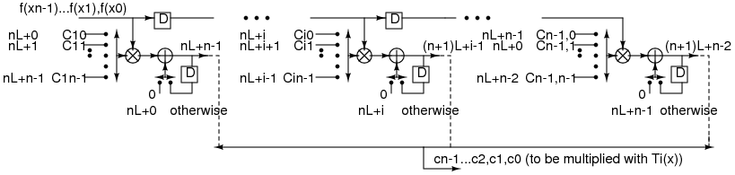
Figure 1: Part of the proposed structure, working on word serial data ${f(x_{i})}$ from a data converter to get the coefficients.

For both, coefficient generation and Chebyshev polynomial evaluation, multiplexers with timing control are used to achieve correct flow of data. For example, the output of the Chebyshev polynomial evaluation unit has to switch between IIR filter mode and connect ‘$0$’ and input ‘$x$’ to the output when $T_{0}(x)$ and $T_{1}(x)$ are evaluated in each $N$ cycle period. Note that since the normalized Chebyshev function values are needed, the recursions are slightly different from Equation 1. For example, even though $\bar{T}_{0}(x)=\frac{1}{\sqrt{2}}$ and $\bar{T}_{n>0}(x)=T_{n>0}(x)$, the recursion formulae for $\{T_{i}(x)\}$ will not work for $\{\bar{T}_{i}(x)\}$. Specifically it will fail at the step where $\bar{T}_{2}(x)$ is substituted as $2x\bar{T}_{1}(x)-\bar{T}_{0}(x)$ since, $\bar{T}_{2}(x)=T_{2}(x)=2xT_{1}(x)-T_{0}(x)$ and $T_{0}(x)$ is different from $\bar{T}_{0}(x)$.

A tabulation of multiplications, additions and computations per cycle required by the word-serial architecture proposed compared to Zhu’s systolic arrays is provided in Table I. Solutions by Wang et al. [9] and Cuypers et al. have not been compared because the former optimizes for a specific output node set and the latter does not discuss the structures at an implementation level.

Architecture	Zhu	Zhu	Proposed
	(time	(transform	(1-Dim
	domain)	domain)	systolic)
Buffering required for	samples	$T_{i}(x)$	none
(memory)	& $T_{i}(x)$
I/O type	word	word	word
	parallel	parallel	serial
Computation of coefficients	$\{\Phi_{i}(x)\}$	$\{c_{i}\}$	$\{c_{i}\}$
Peak operations$/$cycle	$>$8,stored	8	8
Computation of $T_{i}(x)$
Peak operations$/$cycle	0	stored	8
FIR Filtering ($\sum c_{i}T_{i}(x)$)
Peak operations$/$cycle	8	8	8
Latency (cycles)	16	16	16
Hardware Util. Efficiency	100($\%$)	100($\%$)	100($\%$)

TABLE I: Computations needed in different structures (assuming a set of 8 samples).

IV Advantages of Chebyshev sampling

IV-A Reduction of interpolation error

Two characteristic signals are taken to investigate the effectiveness of the interpolation scheme. In addition to a bandlimited signal, a non bandlimited signal ($e^{-x}sin(8x)$) is also chosen. When the number of samples is 8 and the bandlimited function is a sinusoid plus its third harmonic ($sin(4x)+0.5sin(8x),x\in[-1,1]$), the interpolation error for the equispaced case is $\sim$4 times the Chebyshev case as shown in Figure 2. A similar result is obtained for the non bandlimited case as shown in Figure 3.

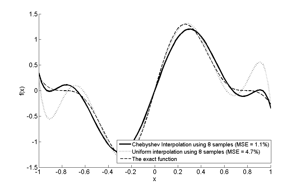
Figure 2: In general, more number of samples for the equispaced case are required in the same interval to reduce the interpolation error.

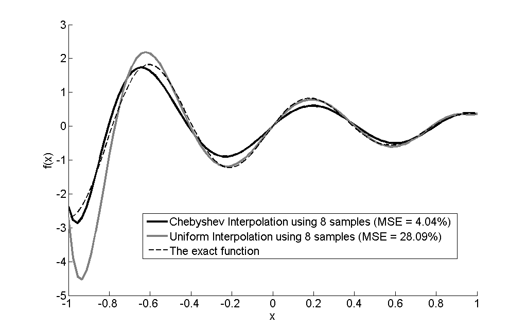
Figure 3: A non bandlimited function $e^{-x}sin(8x)$ over the interval $[-1,1]$ is interpolated using both the schemes.

IV-B Use of Hybrid ADC for power savings

Power savings can be achieved during sampling in a Chebyshev based interpolation system through the use of two (dual) data converters (ADCs) as a hybrid. When the interpolation error limit is fixed for the equispaced and Chebyshev cases, the number of samples required to do so also becomes fixed. In some cases as seen in Section IV-A, equispaced system requires more samples than the Chebyshev system. For the Chebyshev system, a scheme is proposed where the samplings are split between two ADCs, one of which is faster but power consuming (flash) and the other is slower but power saving (SAR). To do so, a flash and SAR ADC are bundled together with a timing control unit to make a hybrid unit. A simple strategy to split the samples between the flash and SAR is based on whether the ratio of the intersample interval is greater than the SAR sampling and conversion time (i.e., $T_{SAR}<floor(sin\mbox{kc}/sin\mbox{c})$ where $c=\frac{\pi}{N+1}$ (derivable from Equation 5). Table II shows the power savings as a function of sharing of samples between the two ADCs for the two example signals of Section IV-A. Note that, Flash ADC topology is assumed to be thermometric (not necessarily the case) and power consumption per comparison in either case is taken to be 1 arbitrary unit (au.)

ADC unit	8 bit Flash	8 bit Flash-SAR hybrid
Interpolation	Equispaced	Chebyshev
To have interpolation error $<1.1\%$ for $sin(4x)+0.5sin(8x)$
Num. of points required	10	8 ($a_{flash}+a_{SAR}$)
Splitting	–	$a_{flash}=6$, $a_{SAR}=2$
Power (au)	$10*2^{8}=2560$	$6*2^{8}+2*8=1552$
To have interpolation error $<4.1\%$ for $e^{-x}sin(8x)$
Num. of points required	11	8 ($a_{flash}+a_{SAR}$)
Splitting	–	$a_{flash}=6$, $a_{SAR}=2$
Power (au)	$11*2^{8}=2816$	$6*2^{8}+2*8=1552$

TABLE II: Sampling power savings per window is $\sim 39\%$ and $\sim 44\%$ resp. for each of the signals.

IV-C Chebyshev Interpolation and Farrow Structures

Even though Chebyshev Interpolation using a Farrow Structure is described in [6], it assumes that the input signal is in the $\theta$ domain. It is worthwhile to compare the structures for chebyshev interpolation in comparison to the Farrow structure which is widely used for equispaced interpolation even though this kind of polynomial interpolation is ill-conditioned. Farrow structure based interpolation units recently have been ported to perform some special nonuniform interpolations [10] but don’t yield to Chebyshev interpolation because the inter-sample intervals are too diverse in range. The DCT shortcut for the Chebyshev case has made this scheme comparable to the Farrow shortcut [11] based equispaced case.

IV-D Design summary and applications

The non-uniformly spaced nodes in the Chebyshev interpolation require block processing which can be a disadvantage for applications where latency is critical. Further, the sampling times are not only irregular but they also cause sampling intervals to be non rational ratios of each other. This implies that there will always be an error in the sampling time even if a very high frequency timing clock is used. An analysis of the optimal number of sample points to be taken in a Chebyshev window hasn’t been done and was fixed to 8. Nevertheless, this parameter has an effect on the flatness of the system frequency response and on the interpolation error. From an implementation perspective, latency would increase with an increase in this parameter. In a broader context like Chebyshev sampling, seeking out optimal node sets contingent to the class of signals at system input could lead to minimal power consumption and reconstruction errors. But such systems, like Chebyshev hardware will need extra logic for compatibility with the existing equispaced systems. For Chebyshev sampling to work well, the average sampling rate should be two times or higher than the $f_{max}$ of the input signal [1], but this is indeed the case in most DSP systems where the equispaced sampling rate is chosen to be 10-15 times $f_{max}$ as a rule of thumb.

Sampling clock synchronization in DSL modems, timing correction, power efficient sensor networking, sample rate conversion in Software Defined Radio are some of the topics where Chebyshev interpolation can be used (fractional delay filters are already being used). Chebyshev interpolation is superior when accuracy is important. It also fits nicely with signal compression like the DCT compression scheme (where only subset of coefficients containing most of the energy are retained) [2].

V Conclusions

A digital architecture performing Chebyshev interpolation based on systolic arrays assuming word-serial data input is implemented in detail and contrasted with other architectures proposed in literature. This structure has a latency of $2N$ cycles between the input and the interpolated output. Merits of Chebyshev sampling compared to equispaced sampling are then explored. A scheme for Chebyshev sampling using a Flash-SAR hybrid ADC unit is also discussed which results in power savings. By optimally distributing the share of samples which will be sampled by either type of ADC, power consumption of the sampling system is optimized. Once the samples have been obtained (sequentially), these are fed to the word serial systolic array for interpolation in the digital domain. Finally, the paper echoes the point that inexpensive digital computation can allow for system specific optimal node sets (not just Chebyshev and equispaced) leading to arbitrary precision in signal interpolation.

References

- [1] V.-E. Neagoe, “Chebyshev Nonuniform Sampling Cascaded with the Discrete Cosine Transform for Optimum Interpolation,” Acoustics, Speech and Signal Processing, IEEE Transactions on, vol. 38, no. 10, pp. 1812–1815, Oct 1990.
- [2] Y.S. Zhu and S.W. Leung, “Systolic Array Implementations for Chebyshev Nonuniform Sampling ,” Acoustics, Speech, and Signal Processing, 1992. ICASSP-92., 1992 IEEE International Conference on, vol. 4, pp. 177–180 vol.4, Mar 1992.
- [3] L. Fox and I.B Parker, “Chebyshev Polynomials in Numerical Analysis,” Oxford University Press, 1968.
- [4] J.C. Mason and David C. Handscomb, Chebyshev Polynomials , CRC Press, September 2003.
- [5] Zhongde Wang, G.A. Jullien, and W.C. Miller, “Fast Computation of Chebyshev Optimal Nonuniform Interpolation,” Circuits and Systems, 1995., Proceedings., Proceedings of the 38th Midwest Symposium on, vol. 1, pp. 111–114 vol.1, Aug 1995.
- [6] G. Cuypers, G. Ysebaert, M. Moonen, and F. Pisoni, “Chebyshev Interpolation for DMT Modems,” Communications, 2004 IEEE International Conference on, vol. 5, pp. 2736–2740 Vol.5, June 2004.
- [7] Chao Cheng and K.K. Parhi, “A Novel Systolic Array Structure for DCT,” Circuits and Systems II: Express Briefs, IEEE Transactions on, vol. 52, no. 7, pp. 366–369, July 2005.
- [8] D.-F. Chiper, “Novel systolic array design for discrete cosine transform with high throughput rate,” Circuits and Systems, 1996. ISCAS ’96., ’Connecting the World’., 1996 IEEE International Symposium on, vol. 2, pp. 746–749 vol.2, May 1996.
- [9] Zhongde Wang, G. A. Jullien, and W. C. Miller, “On Computing Chebyshev Optimal Nonuniform Interpolation,” Signal Processing, vol. 51, no. 3, pp. 223 – 228, 1996.
- [10] D. Babic and M. Renfors, “Power efficient structure for conversion between arbitrary sampling rates,” Signal Processing Letters, IEEE, vol. 12, no. 1, pp. 1–4, Jan. 2005.
- [11] C.W. Farrow, “A Continuously Variable Digital Delay Element,” Circuits and Systems, 1988., IEEE International Symposium on, pp. 2641–2645 vol.3, Jun 1988.