How Does Radio AGN Feedback Feed Back?

Abstract

The possible role of radio AGN ”feedback” in conventional hierarchical cosmological models has become widely discussed. This paper examines some of the details of how such feedback might work. A basic requirement is the conversion of radio AGN outflow energy into heating of the circumgalactic medium in a time comparable to the relevant cooling times. First, the class of radio AGN relevant to this process is identified as FR-I radio sources. Second, it is argued via comparisons with experimental data that these AGN outflows are strongly decelerated and become fully turbulent sonic or subsonic flows due to their interaction with the surrounding medium. Using this, a three-dimensional time dependent calculation of the evolution of such turbulent MHD flows is made to determine the time scale required for conversion of the turbulent energy into heat. This calculation, when coupled with observational data, suggests that the onset of heating can occur $\sim 10^{8}$ yr after the fully turbulent flow is established, and this time is less than or comparable to the local cooling times in the interstellar or circumgalactic medium for many of these objects. The location of where heat deposition occurs remains uncertain, but estimates of outflow speeds suggest that heating may occur many tens of kpc from the center of the parent galaxy. Recent observations suggest that such radio AGN outflows may become dispersed on much larger scales than previously thought, thus possibly satisfying the requirement that heating occur over a large fraction of the volume occupied by the circumgalactic gas.

1 Introduction

The current successes of cold dark matter cosmologies, and in particular the $\Lambda$CDM models, are well known. These hierarchical models begin with the microwave background fluctuations and proceed forward to reproduce the structure in the Ly$\alpha$ forest at $z\sim 3$ (e.g., Mandelbaum et al. 2003) and continue to evolve the dark matter structure distribution to arrive at results consistent with the power spectrum of the distribution of galaxies at the present epoch (e.g., Tegmark et al. 2004), the fraction of baryons in rich clusters (White et al. 1993), and other notable results. These models follow the evolution of dark matter, and the accompanying galaxies are assumed to form as gas flows into the ever growing dark matter condensations (e.g., White and Rees 1978). The most detailed results describing this structure evolution have come from highly sophisticated numerical simulations that follow the growth of mass fluctuations in the early Universe, such as the Millennium simulation (Springel et al. 2005). However, there are some well known difficulties with these models in that they predict too many faint and too many bright galaxies (e.g., Benson et al. 2003), and in addition they predict that the largest galaxies should be blue and star forming.

These are serious difficulties, and they have been addressed through the use of various assumptions about physical processes that work on scales not resolved by the numerical simulations. These ”semi-analytic” models have addressed the problems at both the dwarf galaxy and the brightest galaxy scales; the issues addressed in this paper involve only the problems associated with the evolution of the brightest galaxies. The problems there are a direct result of the hierarchical nature of the models; minute fluctuations in the very early Universe grow due to continuing dark matter and baryonic infall, and in the context of the models this infall should continue to the present epoch, possibly leading to significant star formation now in the most massive galaxies. Thus in this picture the most massive galaxies would be blue due to the large population of young stars, whereas in fact the largest galaxies are generally seen as ”red and dead” at the present epoch, implying that the most active epoch of star formation occurred earlier (e.g., Madau et al. 1996, Cowie et al. 1996).

To address this problem, one of the most commonly used assumptions in semi-analytic models is that of ”feedback” from the central regions of the galaxy, where energy in some form is produced in sufficient quantity that it can heat the inflowing gas, perhaps stopping or reversing the inflow, and in any case providing enough energy to suppress star formation. Once this has been done, the subject galaxy will then passively evolve, and its aging stellar population will become redder with time until the galaxy colors match the observations. Motivated by the observation of active galactic nuclei (AGN) in many massive red galaxies, several AGN related driving mechanisms for this feedback have been suggested. Radiatively driven winds, AGN driven shocks and mass outflows, QSOs, and radio sources associated with AGNs have all been proposed (e.g., Sijacki et al. 2007). In some instances QSOs have been referred to as ”high luminosity” AGN feedback and radio-loud AGN (or ”radio AGN”) have been called ”low luminosity” AGN feedback. This may not be a meaningful distinction, since many QSOs may well be examples of powerful radio sources that are directed toward the observer, with their collimated emission Doppler boosted to very high luminosities. The use of AGNs, and in particular radio AGNs, as sources of the energy required to suppress star formation in feedback models has appeal because estimates for the total energies of these objects derived from energy equipartition arguments have existed for some time. These minimum energies (from $\sim 10^{57}-10^{61}$ ergs) are, in an integral sense, adequate to provide the needed heating for AGN feedback to work. Moreover, recent estimates of the total energies present in some radio sources tend to lie factors of 10 higher than the estimates based on the equipartition energy present in relativistic electrons and fields (Bîrzan et al. 2008).

Thus the total energies available in radio AGN make these objects viable candidates for powering feedback and for suppressing star formation in massive galaxies, and radio AGN have been incorporated into semi-analytic models that are based on cosmological simulations such as the Millennium Run (e.g., Croton et al. 2006, Bower et al. 2006, Okamoto et al. 2008). For example, Croton et al. (2006) show that a form of radio AGN energy input can not only reproduce the observed truncation of the bright end of the luminosity function, but that it can also possibly suppress accretion and give rise to an old, red population of elliptical galaxies. Radio AGN feedback has also been used to explain the presence of old ”red and dead” galaxies in voids (Croton & Farrar 2008), where environmental effects are much less pronounced. Finally, radio AGN feedback has also been suggested by several authors as a means of suppressing cooling or providing reheating in the cores of rich clusters of galaxies, thereby solving the ”cooling flow” problem and at the same time accounting for the colors of brightest cluster galaxies (e.g, Fabian et al. 2000, Brüggen & Kaiser 2002, Ruszkowski et al. 2004, McNamara & Nulsen 2007).

While the integrated total energies of radio sources are adequate, and sometimes more than adequate (e.g., Best et al. 2006) to provide the needed feedback in semi-analytic models, the key question of ”Does it really work?” remains. Having enough total energy is only the first of several conditions that need to be met. In order for radio AGN feedback to work, this energy contained in the outflowing radio sources must be transferred to the surrounding medium. In order to suppress star formation, this energy transfer has to be fairly efficient, and equally important, for radio AGN feedback it has to be turned into heat, and it has to be distributed over most of the volume of gas in and around the halo of the parent galaxy. Finally, all this has to happen in a time less than the local cooling time or dynamical infall time. Until all of these conditions can be met, the effectiveness of radio AGN feedback in solving significant difficulties with current cosmological models will remain in question. This paper provides a calculation of one way this energy transfer process can work. Section II presents an overview of the physical processes involved in radio AGN feedback, while Section III describes a calculation of the energy transfer during the interaction of a radio source with its environment that covers up to 5 orders of magnitude in scale. The results of this calculation are given in Section IV, and the conclusions are found in Section V.

2 Physical Processes in Radio AGN Feedback

A fundamental property of radio AGN that has a major impact on the issue of feedback is the bipolar nature of the energy outflow. Except for low energy ”compact radio sources”, all radio AGN show this morphology. The degree of collimation can be moderate, with opening angles of the flow of order twenty degrees or so, or it can be extreme, as in the case of the very energetic and highly collimated flows associated with high luminosity radio sources and quasars. This two-sided collimated outflow is the principal obstacle to radio AGN feedback being an efficient and effective mechanism for energizing and heating (or blowing away) the gas in the central regions of the parent galaxy, since the heating and suppression of star formation must occur throughout the central region and not just along the two narrow cones in the vicinity of the radio jets. Thus for feedback to be effective, some processes must be found that transfers energy from the jet to the surrounding medium, converts that energy to heat, and distributes it over most of the volume in the central regions of the parent galaxy. Some possible mechanisms for this energy transfer have been previously suggested, such as shock waves from highly supersonic outflows (Brüggen et al. 2007, Graham et al. 2008) or sound wave dissipation from less energetic events (Sanders & Fabian 2007, 2008). These will be considered in more detail later, but in general shock waves are one-time events that rapidly slow and dissipate in the direction transverse to jet motion, while sound waves may or may not carry enough energy to heat large volumes of gas through their eventual dissipation. More importantly, the process of energy deposition by the sound waves in a magnetoionic medium is not clearly understood in this case, especially with regard to the dissipation lengths.

Clarification of possible feedback processes can be found from the luminosities, morphologies and demographics of the radio AGN outflows. Most extended radio sources can be placed in one of two categories first proposed by Fanaroff & Riley (Fanaroff & Riley 1974). These two classes, FR-I and FR-II, are characterized by different luminosities and by very different radio morphologies. High luminosity FR-II objects are generally characterized by two very highly collimated jets of emission extending over large distances, typically hundreds of kpc, with the jets terminating in regions of high surface brightness (”hot spots”) surrounded by lower surface brightness lobes which often have a ”swept back” or ”bow shock” appearance (e.g. Ferrari 1998, De Young 2002). The morphologies of the lower luminosity FR-I objects are dramatically different, with the highest surface brightness near the nucleus of the parent galaxy and a gradual dimming of brightness along two moderately collimated jets with much wider opening angles than seen in the FR-II objects. These outflows are also often bent or distorted and display a meandering morphology as the flow moves outward. This pattern of radio emission is very suggestive of the slow, subsonic flow associated with plumes and turbulent flows, and it was suggested many years ago (e.g., De Young 1981, Bicknell 1984) that these radio sources were characterized by significant interaction with the surrounding ISM or IGM that resulted in mass entrainment and a deceleration of the AGN outflow as it moves away from the nucleus. It may also be that the original outflow speeds in the FR-I objects are less than those existing in FR-II sources, but in any case the current modeling of these objects usually involves deceleration to subsonic flow, presumably mediated by mass entrainment from the ambient medium (e.g., Laing & Bridle 2002, 2004).

The second key point in considering radio AGN feedback comes from the demographics of FR-I and FR-II radio sources. It has been known for some time that the local space density of extended radio sources is dominated by FR-I objects (e.g., Ledlow & Owen 1996, Owen & Ledlow 1997, Jackson & Wall 1999, Willot et al. 2001), where the local ($z<0.1$) density of FR-I objects is roughly $10^{2}$ times that of FR-II radio galaxies. The local density of FR-I radio sources, and a calibration point for constructing radio luminosity functions (RLF) is about 400 Gpc^-1 (Rigby, Best & Snellen 2008). Due to the rapid decline in the detection of the fainter FR-I objects with distance, the dependence of the FR-I/FR-II ratio with redshift is less clear, but recent surveys and modeling of the RLF out to moderate redshifts of less than 1 suggest that the space density of FR-I objects clearly dominates in the local universe (Willot et al. 2001, Cara & Lister 2008, Donoso et al. 2009). Thus to a very good approximation the ”generic” radio AGN outflow in the nearby universe can be taken to be an FR-I radio source. This may also be the case at moderate redshifts as well, since the previous picture of a constant FR-I space density with cosmic epoch coupled with a rapidly evolving FR-II space density may be overly simple (e.g., Rigby, Best & Snellen 2008). In any case it is clear that ”radio AGN feedback” for redshifts less than one can be taken as ”FR-I AGN feedback”, and henceforth the focus here will be on FR-I objects as sources of radio AGN feedback.

A third observational result that constrains the feedback process comes from radio and x-ray observations of radio sources in rich clusters of galaxies. For the first time since their discovery over thirty years ago, it is now possible to carry out calorimetry of some radio source outflows by using estimates of the $pV$ work done by the outflows in inflating cavities observed in the ICM. (e.g., Bîrzan et al. 2008, McNamara & Nulsen 2007 and references therein.) The role of such cavities as being a signature of radio AGN feedback in clusters has been discussed elsewhere, and the relation of this phenomenon to more general FR-I outflows will be discussed at the end of Section 4. The focus here is on the general problem of radio AGN feedback, both in and out of clusters and groups of galaxies, and the relevant result from the radio source calorimetry in clusters is that it reveals outflow energies that are generally in excess of the equipartition values that were commonly assumed in the past (Bîrzan et al. 2008). These $pV$ values are often an order of magnitude greater than the total energies contained in relativistic electrons and magnetic fields in minimum energy equipartition, and they are consistent with most of the energy residing in the kinetic energy flux of the outflow (e.g., De Young 2006).

With these three observational constraints - the meandering plume-like morphology of FR-I radio sources, the dominance of FR-I objects in the nearby radio AGN population, and the existence of much more energy in the outflows than is required to account for the synchrotron radio emission, the most likely paths for radio AGN feedback become more clearly defined. First, if these outflows are truly subsonic over most of their length, and the morphological data are very suggestive of this, then heating by shock waves is not likely to be a significant energy transfer mechanism in these objects, nor is momentum transfer likely to form a nearly spherical outflowing wind that removes the ambient gas. Second, because there is strong evidence that AGN outflows are relativistic on very small ($\sim$ parsec) scales, the FR-I morphology strongly suggests significant deceleration of the flow. The uniform appearance of the outflows from the nucleus outward without any clear discontinuities together with the spreading of the outflow from the nucleus outward implies that this deceleration process begins near the nucleus and continues more or less uniformly throughout the outflow region within the parent galaxy. Deceleration of the flow means a loss of momentum from the jet via a transfer of momentum from the jet to another medium, with the most obvious candidate being the ambient gas in the ISM of the host galaxy. The most natural and most obvious candidate for this deceleration process is thus entrainment of, and transfer of momentum to, the ambient medium at the interface between the outflowing AGN material and the ISM and galactic halo gas.

In addition to continuous deceleration from entrainment, deceleration of the outflow from its original speed near the galactic nucleus could entail the production of shock waves and subsequent heating, since VLBI observations of AGN suggest very rapid outflow speeds on the parsec and subparsec scales in the innermost regions. However, the propagation of a decelerating supersonic jet into the circumnuclear gas will produce a driven bow-shock configuration that, for uniform flow, is a one-time event. In addition, except for the small angular region near the head of the jet, such shocks are generally weak, oblique, and decelerating. Nonetheless, they probably occur around the initial outflow regions of the jets, and as such they could produce localized heating in the innermost regions of the parent galaxy, especially if the AGN outflow involves multiple outbursts. This process may be at work in outflows in rich clusters such as 3C 84, where deceleration is most dramatic due to the very high ambient densities. Because the total energy involved in these shocks is much less than the kinetic energy of the outflow, and because the focus here is not on AGN in rich clusters, the emphasis here will be on the transport of energy by the outflow itself, with most of the flow deceleration being due to continuous entrainment of the ambient medium.

This entrainment process is mediated through the non-linear development of surface instabilities, most notably the Kelvin-Helmholtz (KH) instability, and it is driven by the large ($\sim 10^{43}-10^{45}$ erg s^-1) kinetic energy flux of these outflows derived from the calorimetry described above. Analytic approximations, laboratory experiments, and numerical simulations have all shown that this instability in shearing flows is essentially inevitable. Incompressible flows, compressible flows, supersonic flows, MHD flows and relativistic shearing flows all show the onset and non-linear growth of the KH instability (e.g., Chandrasekhar 1961, Brown & Roshko 1974, Clemens & Mungal 1995, Aloy et al, 1999, Ryu, Jones & Frank 2000, Perucho et al. 2004, 2007). In the fully non-linear stage of development the instability evolves into a mixing layer dominated by large scale vortex structures that entrain material from both sides of the layer into the layer itself (e.g., Dimotakis & Brown 1976). The thickness of this layer grows as one moves down the jet from the onset of the non-linear phase of the instability, and the growth of the layer is nearly linear with distance along the jet until the jet is fully infiltrated by the layer. At that point a different evolutionary phase begins, as is described in Section 3. For a plane mixing layer, which is a good approximation to the cylindrical mixing layer in a round jet in its initial stages (e.g., Dimotakis et al. 1983, Freund et al. 2000), the initial growth is characterized by a nearly constant opening angle that depends upon the relative flow speeds and the fluid densities as

$$Tan\theta\approx(C/2)(\rho_{j}/\rho_{a})^{-\eta}M^{-1},$$ (1)

where $\rho_{j}$ and $\rho_{a}$ are the densities in the outflow and the ambient medium respectively, and $M$ is the Mach number of the outflow relative to the sound speed in the ambient medium (e.g., Brown & Roshko 1974, Dimotakis & Brown 1976, De Young 1993). Empirical data suggest $C\approx 0.16$ and $\eta\approx 0.5$. Within this growing mixing layer the entrainment proceeds through the initial production of large scale eddies whose diameter is roughly equal to the thickness of the layer, followed by the development of finer scale structures within the eddies as well as merging of the larger scale structures. In other words, the mixing layer becomes fully turbulent. Moreover, the thickness of this turbulent mixing layer grows as one moves downstream along the jet, and eventually the turbulence will penetrate throughout the entire volume of the outflow. From Eq. 1, the distance along the jet from the onset of the non-linear mixing layer to the point of complete infiltration of turbulence into the interior of the jet can be approximated by

$$L_{SAT}\sim(2/C)R_{o}M(\rho_{j}/\rho_{a})^{\eta},$$

where $R_{o}$ is the radius of the jet at the onset of the mixing layer. Beyond this point the flow within the jet is fully turbulent; many experimental examples of such turbulent, decelerated jets can be found (e.g., Dimotakis et al. 1983, Mungal et al. 1992), and within the limits of resolution the outflow from FR-I objects such as 3C 31 is indistinguishable from these experimental results. Thus the FR-I demographics, when combined with the evidence for uniform deceleration in their AGN outflows, the universality of shear driven surface instabilities that entrain mass and provide momentum transfer through the growth of turbulent mixing layers, and the morphological similarities between FR-I outflows and subsonic turbulent plumes all provide evidence that the most common energy outflow associated with radio AGN feedback is that of diverging, subsonic, fully turbulent plumes.

This argument is given further support from a comparison of high resolution radio observations of FR-I outflows with experimental results concerning fully turbulent round jets propagating into a uniform medium. There is considerable evidence that such jets are self-similar flows (e.g., Pope 2000, Hussein et al. 1994), and that these flows all have the same opening angle once self-similarity is established. This angle is about 23-24 degrees, and an examination of radio observations of the FR-I objects 3C 31 and 3C 296 (Hardcastle et al. 2005, Laing et al. 2008) shows that both the north and south jets in these objects are very well enclosed by an opening angle of about 23 degrees ($tan(\theta/2)=0.20$). Once the outflows show sudden divergence or bending this is no longer the case, but in the inner regions of the flow where the ambient conditions are likely to be fairly constant or slowly varying, the agreement with self-similar turbulent jets is remarkable. Elements of this picture have been suggested before, and the first numerical simulation of mass entrainment in astrophysical jets was performed many years ago (De Young 1986); there has since been considerable development of phenomenological models of these flows (e.g., Laing et al. 1999, Laing & Bridle 2002, 2004, Wang et al. 2009).

Because magnetic fields are present in both the AGN outflows and in the ambient medium, possible inhibition of the mixing layer growth by magnetic effects might occur, especially for ”favorable” field geometries where ${\bf B}$ is parallel to ${\bf v}$. However, it is clear that in the context of MHD outflow models, the average kinetic energy density must be much greater than the average magnetic energy density in order for the AGN outflow to occur. (The opposite case of nearly mass-free ”Poynting” jets is discussed in the last section.) In the MHD case the concern is then that very local B field amplification due to turbulence could lead to local field energies sufficient to damp the development of the mixing layer. In this case, detailed 3D numerical MHD simulations of the development of the K-H instability and its fully non-linear growth (e.g., Ryu et al. 2000) show that the flow remains ”essentially hydrodynamic”. Small scale field amplifications do occur, and at late times the amplitudes are comparable to the flow energy densities, but these areas are very localized and do not inhibit the growth of turbulent flow in the mixing layer on the larger scales of energy injection into the turbulence. It is important to note the difference between these dynamic, driven outflows and the much slower, passive evolution of buoyant ”bubbles’ in an intracluster medium, where large scale ICM fields may have an influence on the bubble evolution.

This characterization of radio AGN feedback as turbulent FR-I outflows provides the initial conditions for finding processes that can transform this outflow into widespread heating of the ambient medium. A major advantage of turbulent flows is that the ultimate fate of fully developed turbulent flows is conversion of the turbulent energy into heat. Thus if mass entrainment and the generation of turbulence is the most efficient coupling of the AGN outflow to the ambient medium, then the the natural evolution of that turbulence will provide the most effective heating of the gas in the galaxy by radio AGN outflows. A central issue is how long this conversion takes. The next section provides a quantitative estimate of this time through a calculation of the evolution of a driven turbulent flow from its onset until its dissipation.

3 Evolution of Turbulent AGN Outflows

3.1 Formalism

The turbulent flow that describes the radio AGN outflow can be recast in a form common to many turbulent flows. On some large scale comparable to a defining scale of the problem (e.g., the radius of the outflow) energy is injected in the form of turbulent eddies. This process, as verified by experiment, involves a large scale ingestion of material on both sides of flow boundary in a ”gulping” mode by the largest eddies (e.g., Dimotakis & Brown 1976), followed by a rapid generation of finer and finer structure and mixing within this large scale as the flow evolves to smaller scales. In terms of the evolution of the energy spectrum of the turbulence, this can be described as energy injection over a small range of wavenumber $k$ followed by a loss free cascade of energy to larger wavenumbers. For homogeneous and isotropic hydrodynamic turbulence this process results in the standard power-law Kolmogorov spectrum with $E_{v}\propto k^{5/3}$. (For MHD turbulence the power-law exponent is less well defined but is generally somewhat smaller.) The dissipation of the turbulent kinetic energy into heat occurs at and above some wavenumber $k_{d}$ which generally lies many orders of magnitude above the energy injection scale $k_{I}$. The Kolmogorov formalism describes an equilibrium state where the energy input at $k_{I}$ is exactly balanced by the dissipation at $k_{d}$. The problem being addressed here is not as simple, since what is needed is a calculation of the time required for the flow to reach the dissipation range at $k_{d}$ after the injection has begun at $k_{I}$. Because the evolution of the turbulent flow involves the non-linear interaction and energy transfer among turbulent scales of many different sizes, both upward and downward in $k$ space, the evolution must be calculated explicitly. In addition to the time dependent nature of the flow, a major hurdle is the many orders of magnitude in scale between the size of the large eddy injection range (tens of parsecs or more) to the energy dissipation scale due to effective viscosities in ionized plasma (possibly meters or less).

Some simplifying assumptions can be made. If the overall outflow of the FR-I AGNs is subsonic or transonic relative to the ambient medium, then the flow can be regarded as generally incompressible. In addition, in a frame comoving with the mean local outflow speed the turbulence can be treated as locally homogeneous and weakly isotropic (in that helicity is allowed) to a good approximation. Under these conditions a technique may be used that calculates the three dimensional time dependent evolution of turbulence, both hydrodynamic and magnetohydrodynamic, over several orders of magnitude in spatial scale. The original method was devised to treat purely hydrodynamical turbulence (e.g., Orszag 1970, 1972) but was subsequently generalized to include magnetic fields in the MHD approximation (Pouquet et al. 1976, Pouquet et al. 1978, De Young 1980). This approach takes moments of the Fourier transforms of the equations of mass, momentum and energy conservation in order to obtain equations that describe the time evolution of second moments of velocity and magnetic field, i.e., the kinetic energy and magnetic energy, as a function of time and spatial scale. The system of moments is closed by using a quasi-normal approximation that assumes the fourth order moments are related to the second order moments in the same way as is the case for a Gaussian distribution of Fourier modes. This ”quasi-normal” approximation permits closure of the system of equations at second order and results in differential equations that describe the temporal and spatial evolution in Fourier space of the square of the fluid velocity (i.e., kinetic energy per unit mass) and the magnetic energy per unit mass. The calculation uses a complex form of eddy viscosity that employs a Markov cutoff in ”memory” of the eddy interactions and includes the non-linear transfer of energy among turbulent eddies of different sizes, including triads of eddies with differing wavenumbers. Some additional details are found in the Appendix. The principal advantages of this eddy damped, quasi-normal Markov (EDQNM) method are its ability to calculate the time evolution of the turbulence over very large spatial ranges and its relatively modest computational requirements, especially when compared to the more straightforward methods of direct numerical simulation. The technique is is wide use, and its accuracy has been verified by comparison with both direct numerical simulations and with laboratory experiments (e.g., Gomez et al. 2007, Vedula et al. 2005, Turner & Pratt 2002, Lesieur & Ossia 2000, Staquet & Godeferd 1998).

Details of this technique can be found in Orszag (1977), Lesieur (2008), and Pouquet et al. (1976) and De Young (1980) for the MHD generalization. As discussed in the Appendix, evolution of the turbulence is followed by solving a series of integro-differential equations of the general form

$$(\partial/\partial{t}+2\nu k^{2})E(k)=F(k)+\int T[k,p,q,E(k,p,q)\nu]dpdq.$$ (2)

Here $E$ is the Fourier transformed magnetic or kinetic energy at wavenumber $k$, $\nu$ is a dissipation constant (either viscosity or magnetic diffusivity), $F(k)$ is the forcing function or driving term, which in this case arises from the surface instabilities at the jet-ambient medium interface that create the large scale turbulent eddies driving the turbulent flow. The term $T$ represents the non-linear transfer terms in the flow which mediate the transfer of magnetic and kinetic energies over all wavenumbers; i.e., $T$ describes the processes that create the cascade of energy from large scale to small scales, the amplification of magnetic fields by fluid turbulence, and the inverse cascades, if any, of energy from small scales to larger scales. (Which in general is significant only in the presence of flows with net helicity.) In general all of $E$, $F$, and $T$ are time dependent. The explicit form for $T$ can be complex because it describes the interaction of hydrodynamic turbulent eddies with each other, the interaction of hydrodynamic turbulence with any magnetic fields and the resulting possible magnetic field amplification, the effects of eddy viscosity, and the self interaction of magnetic turbulent structures with each other. The complete MHD forms of $T$, including the effects of helicity ($v\cdot\nabla\times v$ and its magnetic counterpart $b\cdot\nabla\times b$) are given in De Young (1980).

In the present case magnetic effects are not of major concern. However, a very small, dynamically unimportant magnetic field is included for completeness; its initial energy density is $10^{-2}$ that of the turbulent kinetic energy density. It could in principle play a role in the dissipation process at small scales, but to include these effects would require a knowledge of the detailed field reconnection and dissipation mechanisms, which in turn would require a specification of field geometries and strengths as a function of scale length. Since these are unknown, the magnetic diffusivity is chosen to be consistent with the hydrodynamic dissipation as described below. Magnetic field amplification to equipartition with the hydrodynamic energies will occur on very small scales, but in the absence of any helicity this will have no effect on the evolution of the turbulence on the scales of interest here.

The problem is specified by the injection of kinetic turbulent energy at some rate $F(k)$ at a scale defined as the energy range, and the evolution of the turbulent energy spectrum is then followed as the energy cascades to smaller and smaller scales. A natural unit for length is that corresponding to the energy injection scale, $L_{o}\propto 1/k_{I}$, and a corresponding time scale comes from the largest eddy turnover time; i.e., $t_{o}\approx L_{o}/v_{o}$, where $v_{o}$ is the mean velocity of the turbulent flow. Because the turbulence is driven by shear instabilities in the mixing layer between the AGN outflow and the surrounding medium, $v_{o}$ is comparable to the local jet outflow speed. The calculations here are basically scale free. This is because the actual dissipation scale is very many orders of magnitude smaller than the energy injection scale, and inclusion of the energy scale, which is necessary, means that even with this technique the calculation cannot span the scale lengths from energy injection to dissipation. The dissipation scale is given by $k_{d}\approx k_{I}R^{3/4}$, where $R$ is the Reynolds number appropriate to the large scale flow and $k_{I}$ is the wavenumber corresponding to the energy injection scale. The hydrodynamic Reynolds number is $R=<v_{I}^{2}>^{1/2}/\nu k_{I}$, where $<v_{I}^{2}>^{1/2}$ is the average velocity at scales $k_{I}$; i.e., $v_{I}\sim v_{o}$. The magnetic Reynolds number is just this expression with the magnetic diffusivity $\lambda$ substituted for the kinetic viscosity $\nu$. For a hot ($\sim 10^{7}$K) rarefied ($n\sim 10^{-4}$) plasma $\nu\sim 10^{-4}$ (e.g., Spitzer 1962), and energy injection scales of tens of parsecs and sonic or subsonic flow speeds of $10^{2}-10^{3}$ km/sec imply ten or more orders of magnitude in scale between the energy injection scale and the dissipation scale. Even though the equations of the form (2) above are solved numerically on a logarithmic scale in $k$ space, a solution that spans the complete scale from $k_{I}$ to $k_{d}$ is not feasible, especially in view of a causality condition discussed below. Thus the actual values of the dissipation constants $\nu$ and $\lambda$ never enter into the calculation, and no inherent scales are present. This means that application of the results can be applied to many different spatial and time scales, and this characteristic will be used in estimating the time for the turbulent energy flow to actually reach the regime where energy is dissipated into heating the ambient medium.

Because the wavenumber range included in the calculations is less than the complete range to $k_{d}$, some mechanism has to be used at the upper end $k_{top}$ of the calculated wavenumber range to simulate the continuation of the loss free cascade of energy to wavenumbers beyond $k_{top}$. If this is not done, unphysical reflection of turbulent energy from the upper end of the calculated wavenumber range can occur. A standard method for treating this is to use artificially large values of the dissipation constants $\nu$ and $\lambda$. These are adjusted so that the resulting effective values of $k_{d}$ are somewhat less than $k_{top}$ so that no spurious energy reflections are seen. The differential equations of the form given by Eq. 2 are solved numerically on a discrete grid in $k$ space, and in order to avoid non-physical energy fluctuations, a time step control similar to a Courant condition must be used. The value of the time step in the integration is chosen to be less than the minimum of $[1/(v_{I}k_{top}),1/(k_{top}^{2}\nu)$. This ensures the correct behavior at high wavenumbers; it also illustrates why extending the calculated wavenumber range beyond about 5 orders of magnitude is not practical. Because the calculation is scale free, the obvious scaled values to choose are $k_{I}=1$ and $v_{I}=1$; once the physical dimension and speed corresponding to these are chosen, the time step is determined and the problem is well defined.

The scale-free nature of the calculation allows a simple estimate of the time required to actually reach the true dissipation range once a calculation has reached equilibrium over the more limited wavenumber range described above. Suppose a calculation is made of the evolution of the turbulence spectrum between some $k_{1}$ and $k_{2}$ using a $\delta$-function energy input at $k_{1}$. Let $k_{2}$ be some large multiple $M_{1}$ of $k_{1}$, about 100, and suppose the spectrum reaches a steady state at some time $t_{1}$, where $t$ is measured in units of $t_{1,o}=\ell_{1}/v_{1}$ with $\ell_{1}\sim 1/k_{1}$; $t_{1,o}$ is roughly the large scale eddy turnover time at $k_{1}$, and $v_{1}$ is the mean flow speed of the turbulence on this scale. Hence $t_{1}$ can be measured in units of the turnover time and thus $t_{1}\approx N_{1}t_{1,o}$. Because it is scale free, the same calculation also applies to driving turbulence between $k_{2}$ and $k_{3}=M_{2}\times k_{2}$ with a $\delta$-function at $k_{2}$. In this case a steady state is reached in some time $t_{2}$ where now $t$ is measured in units of $t_{2,o}=\ell_{2}/v_{2}$ with $\ell_{2}\sim 1/k_{2}$. Similarly, the calculation can be made between $k_{3}$ and $k_{4}=M_{3}\times k_{3}$, and so on until some $k_{n}$ is reached where $k_{n}\approx k_{d}$. Then the total time required for the turbulence to cascade from $k_{1}$ to the dissipation range is just $t_{d}=t_{1}+t_{2}+t_{3}+...+t_{n}$. But $t_{1}=N_{1}t_{1,o}=N_{1}\ell_{1}/v_{1}$ and similarly for the other $t_{i}$. But in this scale-free calculation, $M_{1}=M_{2}=...=M_{n}=M$, and thus $N_{1}=N_{2}=N_{3}=...N_{n}=N$, and so $t_{d}=N(\ell_{1}/v_{1}+\ell_{2}/v_{2}+...+\ell_{n}/v_{n})$. To a first approximation all of the $v_{i}$ are equal, though it could be argued that as one goes to smaller and smaller scales the relevant values of $v_{i}$ decrease due to an increasing effective viscosity, especially in the presence of magnetic fields. By setting all $v_{i}=v_{1}$ a lower limit on the value of $t_{d}$ is obtained, and this is the most constraining value for the issue of concern here. Then $t_{d}\approx(N/v)\Sigma\ell_{i}$, and since $\ell_{i}\sim 1/k_{i}$ the time for the turbulent flow to reach the dissipation range and begin to heat the ambient medium is

$$t_{d}\simeq(N\ell_{1}/v)[1+1/M+1/M^{2}+...+1/M^{n-1}].$$ (3)

Thus a good approximation of the time for the turbulent cascade to reach the dissipation stage is just the number $N$ of large scale eddy turnover times that are required for the establishment of a steady state turbulent cascade over a factor of about $M\approx 100$ in scale and beginning with the scale of the large scale energy injection. i.e., $t_{d}\approx N\ell_{1}/v_{1}$.

3.2 Initial Conditions

In this model the energy injection occurs on the scale of the largest eddies when the outflowing jet first becomes fully turbulent from outer boundary to centerline. In the limiting case the energy injection spectrum could be taken as a delta function centered on $k=k_{I}=1$, and the energy injection function in Eq. 2 would have the form $F(k)=F_{v}\delta(k=k_{I}$). Since the goal of the calculation is to determine the time required for the turbulence originating on a scale $k_{I}$ to cascade down to the dissipation range, the injection spectrum should be some sharply peaked function centered on $k_{I}$. A narrow Gaussian form may be more cosmetically appealing but will be seen to have little effect on the outcome of the calculation. The value of the constant $F_{v}$ controls the amplitude of the energy injection spectrum, and because the calculation is looking at the minimum time required for the turbulent cascade to reach the dissipation range, values of $F_{v}$ near the maximum allowed are of interest. The units of $F_{v}$ are (kinetic) energy per unit mass per unit time, and in the dimensionless units used here, $F_{v}$ should be some fraction of $v_{I}^{3}/R_{t}$, where $R_{t}$ is the value of the jet radius at which the flow becomes fully turbulent throughout its volume. The maximum value of $F_{v}$ is then equal to one. A ”reasonable” choice might be to set an average large scale eddy size to half $R_{t}$ and the similarly for some average rotation speed of those eddies as $v_{I}/2$, which gives a value of $F_{v}=0.25$ in dimensionless units where $v_{I}=1$ and $R_{t}=1$. In fact, it will be seen that values of $F_{v}$ between 1.0 and 0.1 yield roughly the same results. Introducing a time variation in $F_{v}$ is easily done, but such variations could only be less than the maximal value and thus defeat the purpose of finding minimum equilibration times. Hence $F_{v}$ will be kept constant.

A major virtue of the formalism used here is that the calculation is carried out with logarithmic intervals in $k$ space, and though this introduces some complications to ensure that energy transfer among structures in neighboring regions of wavenumber space is not incomplete, it allows the calculation to cover many orders of magnitude in scale and thus permits the development of a turbulent cascade through the loss-free inertial range. In general the calculations here cover almost four orders of magnitude in scale in three dimensions, which would require a major computational effort in a direct numerical simulation. Most calculations used a wavenumber range of $k\in[0.015,128]$, while more extensive runs extended the upper limit to $k=1024$. The kinetic energy in the EDQNM formalism must be positive definite, so the initial energy spectra were set equal to a constant but negligible value of $10^{-4}$ in scaled units at all wavenumbers. This is three to four orders of magnitude below the injection energy and has no effect on the evolution of the energy spectrum resulting from the turbulent mixing layer. The energy levels at the upper and lower ends of the wavenumber range were not fixed after initialization. In practice there is no significant inverse cascade of energy in the absence of helicity, so the value of $E_{v}$ at the low end of the wavenumber range (largest scale) does not evolve from its initial value. The energy at the largest wavenumber $k_{top}$ begins to fall immediately due to the very rapid energy transfer on the smallest scales, but this value always remains non-zero.

3.2.1 Parameter Space

The major free parameters in these calculations are the shape and amplitude of the energy injection spectrum $F_{v}(k)$. Other parameters that can be varied are the wavenumber range, the length of time covered by the calculation, the value of the viscosity to test for any influence on the spectral evolution, and the density of points in wavenumber space. For most of the calculations the shape of $F_{v}(k)$ was taken to be a delta function centered at the energy injection scale $k_{I}$, as discussed above. In some runs this shape was changed to a Gaussian distribution in the log of injection energy sharply peaked at $k=k_{I}$, and with $\sigma=0.2$ in log$k$. The values of $F_{v}$ ranged from the maximum of 1.0 to 0.01, with the most common value being 0.25 as described previously. The normalization constant for the Gaussian runs was chosen so that the peak of the distribution had the same amplitude at $k=k_{I}$ as did the delta function energy injection, thus providing a comparable energy injection rate. The scaled wavenumber range was in most cases from 0.015 to 128, with a few runs being made over the range $k\in[0.015,1024]$. Values of the time evolution of the turbulent energy spectra were calculated at equally spaced logarithmic intervals in the $k$ domain; some runs were repeated with the density of points increased by a factor of two to see what effect, if any, would result from changing the size of $\Delta k$. As described above, values of the viscosity $\nu$ were chosen so that an effective $k_{d}$ lay near the value of $k_{top}$. Various small changes in $\nu$ were made in some runs to find the smallest value of $\nu$ that would not produce any ”feedback” from the upper end of the $k$ range into the larger scales. Such unphysical inverse cascades were immediately apparent by the growth or ”bunching up” of elevated $E_{v}$ values at the top end of the wavenumber range. Adequately high dissipation to ensure only a direct and unimpeded cascade to smaller scales (large $k$) was always shown by a rolloff in values of $E_{v}$ from a power law at the highest wavenumbers. The timestep was determined for each run via the effective Courant condition described earlier; increases in $\Delta t$ much above this value immediately result in zero or negative values of $E_{v}$ at the highest wavenumbers.

4 Results

The objective of these calculations is a determination of the time elapsed from the onset of driven turbulence on some large scale to the transformation of the turbulent energy into heat at the dissipation scale. This first occurs when the turbulent cascade reaches an equilibrium or steady state condition with energy flowing in at $k_{I}$ and being dissipated at $k_{d}$ after transit through a loss free cascade to ever smaller scales. Establishment of this equilibrium is an asymptotic process, hence the time required for equilibrium will be set at that time when any changes in the energy spectrum per unit time are less than a few percent. This will give a minimum time for establishment of equilibrium and will result in the minimum time for feedback into heat to occur.

The approach to equilibrium is slightly complicated because there is no well defined ”front” of energy marching down to smaller scales into a constant background of very low turbulent energy. Instead, as soon as the calculation is begun, energy begins to flow to higher wavenumbers, as it should. This means that the initial constant and very small value of $E_{v}$ set at the beginning shows a decay at large $k$ before the energy flow from the injection region arrives at the smallest scales. Hence the shape of the spectrum evolves over the

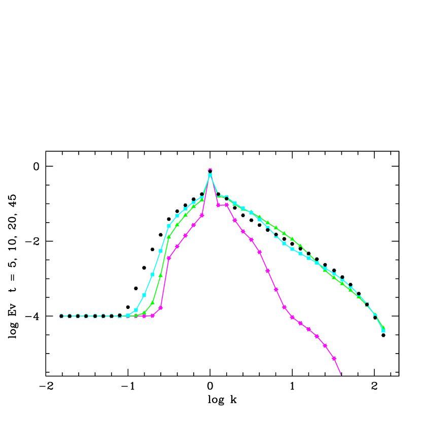
Figure 1: Early time evolution of the turbulent kinetic energy spectrum. Energy is injected with a delta function at $k=1$, and time is measured in units of eddy turnover time at $k=1$. Magenta stars: t=5; green triangles: t=10; blue squares: t=20; black circles: t=45. The spectrum has not reached equilibrium by $t=45$.

full wavenumber range for all times greater than zero. Figure 1, which shows the early evolution of the turbulent kinetic energy spectrum as a function of time, illustrates this behavior. In this case the energy injection spectrum has a delta function form for $F(k)$ at $k=1$, and time is measured in units of the $k=1$ eddy turnover time, $t_{o}=R_{t}/v_{I}$. At early times ($t\leq 5$) the effects of the energy drain at large wavenumber is very evident, since the spectrum in this range is reduced far below the initial constant value of $10^{-4}$ described in Section 3.2. Nonetheless, at $t=5$ the flow of energy from the injection region at $k=1$ to smaller scales is clearly seen, with a ”front” of the energy cascade having arrived as far as $k\approx 10$. By $t=10$ the effects of energy injection have reached to scales of order $10^{-2}$ smaller than the injection region, but, as Figure 1 shows, the spectrum has not yet reached an equilibrium state by $t=45$. Figure 2 shows the late time evolution of the kinetic energy spectrum, and there it is clear that for scales smaller than the injection scale, there is very little evolution in the spectrum at times later than $t=60$, with little or no evolution past $t=100$. At larger scales there continues to be a slow growth of turbulent energy on scales of up to 10 times the size of the injection region, consistent with previous calculations. However, this region is of no concern for the present problem, and in addition the applicability of homogeneity on these scales is less certain for the jet structures considered here. The region $k<1$ has no effect on small scale evolution, and in the absence of helicity almost all the injected energy cascades to the small scale regions (e.g., De Young 1980).

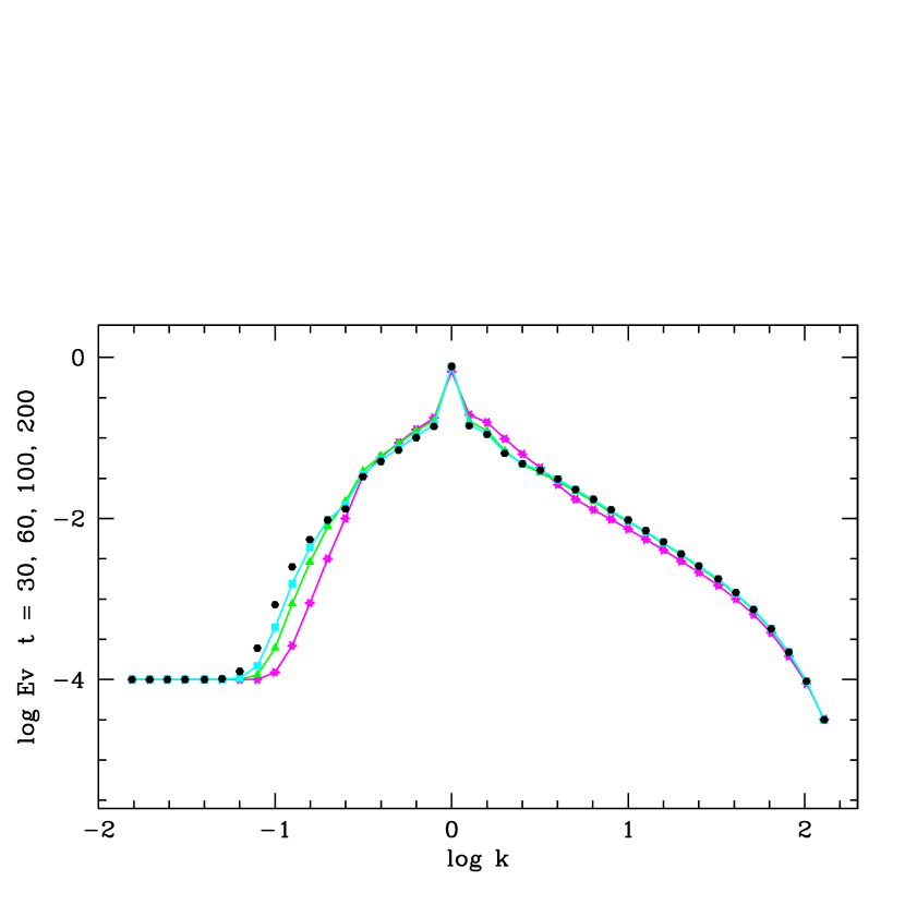
Figure 2: Late time evolution of the kinetic energy spectrum shown in Figure 1. Magenta stars: t=10; green triangles: t=60; blue squares: t=100; black circles: t=200. The spectrum has reached equilibrium by $t=200$ for all values of $k\geq 1$.

Figure 3 shows the resultant spectrum at $t=60$ when the wavenumber space is extended to $k=1024$, thus spanning over 5 orders of magnitude in scale. As discussed above, this is a practical maximum for a single calculation due to the time step constraints at the smallest scales. Figure 3 also shows a comparison between a $\delta$ function energy injection at $k=1$ and a Gaussian energy injection on the same scale with the normalization discussed in the previous section. It is clear that there is no significant difference in the late time spectra that result from the two different energy injection functions. Also evident in Figure 3 is the establishment of a clear power-law energy spectrum for times greater than

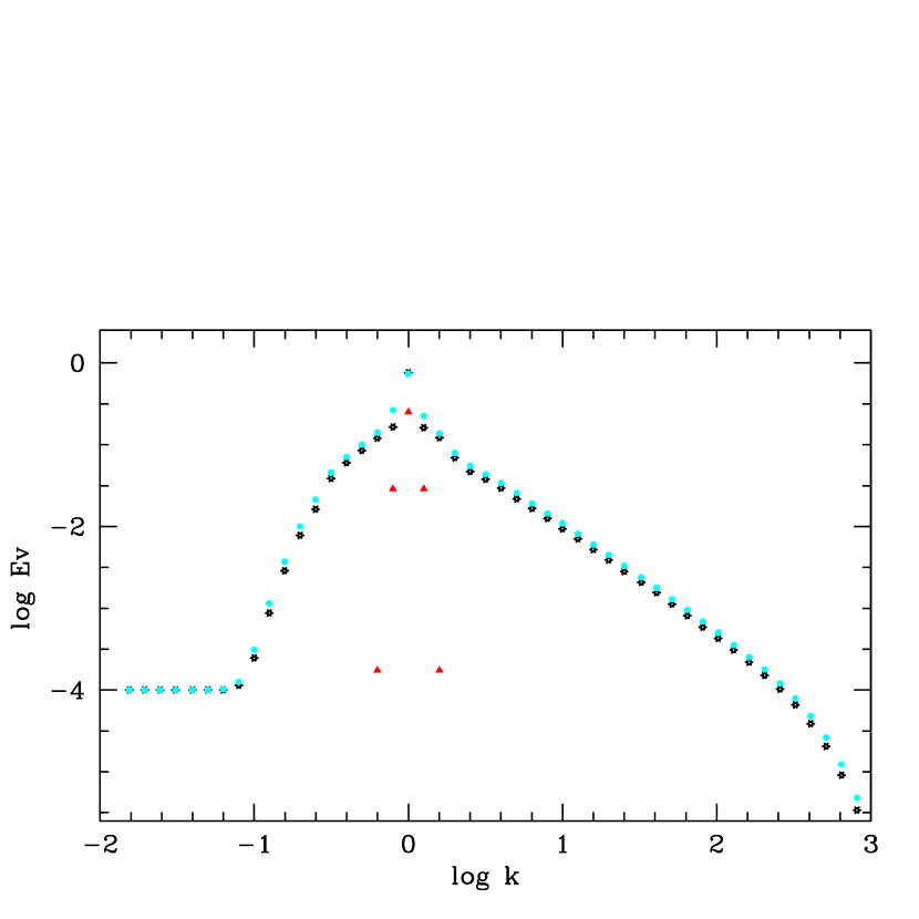
Figure 3: Turbulent kinetic energy spectra at a scaled time of $t=60$ for a wavenumber space extending to $k=1024$. Shown are the spectra for delta function (black) and Gaussian (blue) energy injection profiles, with the form of the Gaussian injection spectrum also shown by red triangles. No appreciable differences exist in the overall energy spectrum for the two different injection profiles.

$t=60$. Finally, Figure 4 shows the time evolution of the total (kinetic plus magnetic) energy for the $\delta$ function injection case that covers the range $k\in(0.015,1024)$. From this figure it is clear that the turbulence has not reached an equilibrium state for times less than $t\simeq 70$. However, it does seem that equilibrium is established by $t=100$. The early rapid growth of $E_{tot}$ for times less than ten is due to the constant inflow of injected energy with no loss at the high wavenumber end having yet occurred. The slower growth for $t>10$ reflects the evolution of the spectrum after energy loss begins but is not yet in equilibrium. In addition, after $t=10$ the conversion of kinetic energy into magnetic energy begins to become noticeable at the few percent level. Throughout all these calculations, the total turbulent energy is always dominated by the kinetic energy; the maximum magnetic energy integrated over all scales never exceeds about 70 percent of the kinetic energy.

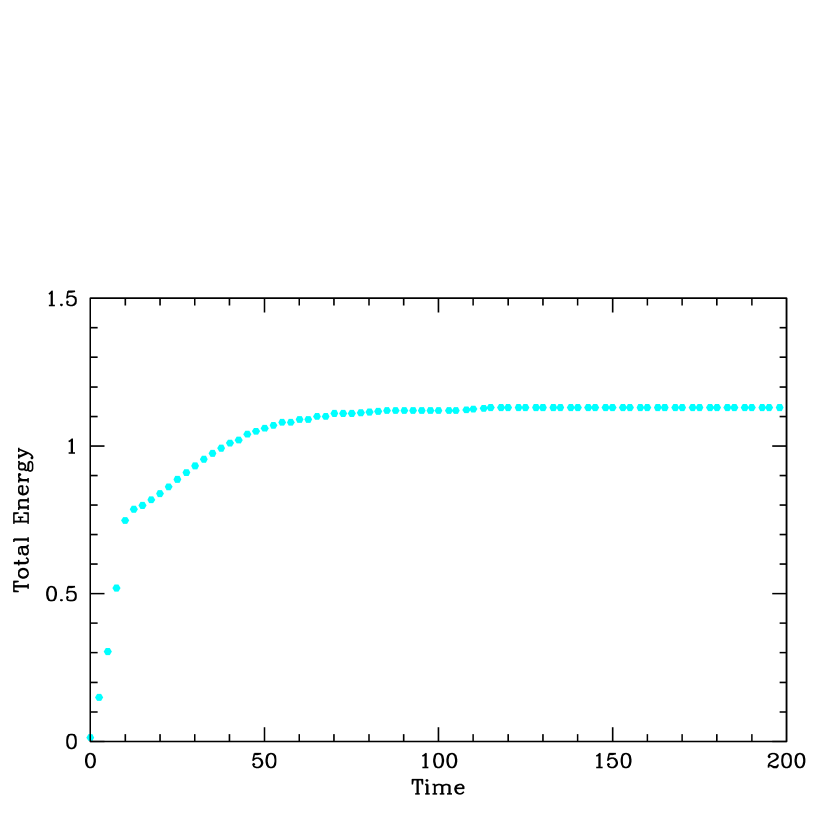
Figure 4: Time evolution of the total (kinetic plus magnetic) turbulent energy for the extended ($k_{top}=1024$) case and delta function energy injection. Irregularly spaced data are due to plot roundoff. The evolution of $E_{tot}$ is discussed in the text.

Additional calculations were made with variations of other parameters mentioned in the previous section, such as variation of $F_{v}$, $\Delta k$, $\Delta t$, $k_{max}$, and $\nu$. However, these variations did not significantly alter the overall results presented in Figures 1 though 4. In particular, the variation of $F_{v}$, which might be thought to have the largest effect, was not particularly notable. Calculations were made with values of $F_{v}$ varying from 0.1 to 1.0, and while the amplitude of the turbulent energy spectrum increased as $F_{v}$ was increased, the shapes of the equilibrium spectra were virtually invariant over an order of magnitude change in $F_{v}$. This is not surprising given the tendency for the turbulent MHD cascade to evolve toward a common power-law form. Moreover, the scaled time required to establish equilibrium was about $t\approx 100$ in all cases, which is consistent with a scale free calculation. Variations in $\Delta t$ and $\nu$ have been discussed above; these are controlled by the Courant condition to preserve positive definite energies and to avoid unphysical inverse cascades of energy at large wavenumber. The effects of changing the upper limit on the wavenumber range are shown in the figures; a more clear definition of the loss-free power-law energy cascade is seen with larger $k_{max}$, but the time required to reach equilibrium is not affected. This is also an expected result, since equilibrium is reached most rapidly at the smallest scales (largest $k$). Decreasing the value of $\Delta k$ and increasing the density of computational points has the expected effect of making the energy transfer among triads of wavenumbers slightly more efficient. A doubling of the density of points in $k$ results in maximum change in $E_{v}$ of 7 percent at the upper end of the wavenumber range. Again, the time to reach equilibrium, which is governed by processes on the larger scales, is unaffected.

Thus a robust conclusion that emerges from these calculations and which is illustrated in Figures 2 and 4 is that the turbulent cascade reaches equilibrium over the wavenumber range $k\in(.01,1000)$ in about 100 large scale eddy turnover times; $t_{eq}\approx 100t_{o}$. This result can then be combined with Equation 3 for the time required after the onset of energy injection to reach turbulent dissipation of energy into heat;

$$t_{d}\approx(N\ell_{1}/v)[1+1/M+1/M^{2}+...+1/M^{n-1}]\\ \approx(N\ell_{1}/v).$$

Thus these results imply that a value of $N=100$ is appropriate for these turbulent jet flows. With this result in hand it is now possible to estimate the time required for radio AGN outflows to convert their outflow energy into heat. To do this requires a conversion from the scale free calculation here into the relevant astrophysical quantities.

4.1 Scaling

The first scale to establish is the spatial scale that corresponds to $k_{I}$ where the energy is injected. This is basically the size of the large scale fully developed turbulent eddies which are driving the turbulence, powered by the vorticity generated in the shearing motions of the mixing layer. As described earlier, the mixing layer grows in thickness until it permeates the entire jet, at which point the flow is fully turbulent, and it is at stage that the interior of the jet can be characterized as a homogeneous and isotropic (in a comoving frame) turbulent flow. Hence the size of the large scale eddies at the point of complete turbulent infiltration or saturation is an appropriate measure of the energy injection scale. Given the internal structure of mixing layers, a good approximation for this eddy size is just the radius of the outflowing jet at saturation, since that is where the linearly expanding mixing layers merge together and the potential flow in the core of the jet ceases. Experimental data on gaseous turbulent jets also show that the large scale structures at this point are comparable to the jet radius (Dimotakis et al. 1983). In addition, it is at this point that the opening angle of the outflow increases slightly and takes on the common value of $tan(\theta/2)\approx 0.2$ seen in fully turbulent round jets. (Some experimental data for turbulent jets also show the creation of larger scale structures that develop in the downstream flow, but these are often attributed to merging or pairing of large eddies formed earlier rather than an indication of an energy injection scale (e.g., Brown & Roshko 1974, Dimotakis et al. 1983). In addition, these structures are most apparent in fluid turbulent jets and are less dominant in very high Reynolds number gaseous jets (Dimotakis et al. 1983, Dahm & Dimotakis 1990).) Determination of the jet radius when it becomes fully turbulent can be estimated from analytic approximations to $L_{sat}$ or from observations of the early stages of FR-I outflows. The latter is probably the more robust method, given the uncertainty in the initial jet densities and outflow speeds. Radio observations of the inner regions of 3C 31 and 3C 296 (Hardcastle et al. 2002, Laing et al. 2008, Hardcastle et al. 2005) permit an estimation of the jet width in its earliest turbulent phase. In particular, the southern jets in these objects show an increase of the jet opening angle to $\sim 25$ degrees that marks the transition to self-similar fully turbulent outflow. Estimates of the jet radii at these points give values in the the range $\approx 0.14-0.17$ kpc, and thus a reasonable estimate from these data for the scale corresponding to $k_{I}$ is about $0.1-0.2$ kpc.

A consistency check can be made by looking at the corresponding values of $L_{sat}$ and the density ratios and outflow speeds that would be required. For example, in 3C 31 the estimated point where the jets appear fully turbulent is at a distance of about 1.7 kpc from the nucleus, while in the case of 3C 296 this distance is about $1.5$ kpc. Using this as a rough measure of $L_{sat}$, and assuming that the functional form for plane mixing layers given above can be generalized to mixing layers for round jets, given the overall similarity of the mixing layers in the two cases (e.g., Freund et al. 2000, Dimotakis et al. 1983), then it is possible to see if ”reasonable” values of outflow densities and speeds near the nucleus result. The jet becomes fully turbulent at a radius $R_{t}\approx 2R_{o}$, and using $\eta\approx 0.5$ and $R_{t}\approx 0.15$ kpc as an average of the above numbers, together with the observed temperatures and inferred number densities for the ambient medium in 3C 31 and 3C 296 at about 1.5 kpc from the their nuclei (Hardcastle et al. 2002, 2005) gives jet flow speeds in the innermost regions of $\sim 10^{9}$ cm s^-1 and jet number densities of $\sim 10^{-5}$ cm^-3, This is consistent with models of ”light” jets which are mildly relativistic in the innermost regions (e.g., Laing et al. 2008). Thus different and independent approaches indicate that a value of $R_{t}\sim 0.15$ kpc is a consistent value to take for the scale of the energy injection range, and this value will be taken to be the size corresponding to $k_{I}$.

Once a value of $R_{t}$ is established, the remaining scales can be fixed by setting a velocity scale, and this is usually chosen to be the turbulent turnover speed of the large scale eddies in the energy range. The flow in the mixing layer is subsonic relative to the ambient medium as argued previously, perhaps transsonic at most in the initial stages. Hence the value of the eddy turnover speed $v_{I}$ will be some fraction of the local sound speed in the ambient medium, and this in turn has been established for some FR-I objects via observations of x-ray emission in the central regions of the parent galaxies. These observations are consistent with thermal bremsstrahlung radiation, and thus a temperature and sound speed for this gas can be established. In particular, Chandra observations of 3C 31 and 3C 296 (Hardcastle et al. 2002, 2005) are consistent with gas temperatures of order $10^{7}$K, with corresponding sound speeds of $\sim 3\times 10^{7}$ cm s^-1. Thus a an average value of $v_{I}\approx 10^{7}$ in the energy injection range is consistent with observations and will be used here. This value is significantly less than the above estimate of $10^{9}$ in the innermost region of the jet, and so it is also consistent with significant deceleration having occurred, especially in the outer layers of the jet, due to mass entrainment via the growing turbulent mixing layer. Once these scales are established, a time unit of $t_{o}\approx R_{t}/v_{I}$, the large eddy turnover time, follows naturally, as does the unit of turbulent kinetic energy density per unit mass, $v_{I}^{2}$. This last quantity is the unit (per unit wavenumber) used in the energy spectra shown in Figs. 1-3.

4.2 Radio AGN Feedback

The previous two sections provide the information needed to establish an estimate of the time required from the establishment of a fully turbulent outflow in an FR-I jet to the onset of conversion of turbulent energy into heat. As argued above, both observations and analytic approximations suggest a large scale eddy size at the energy injection region of $R_{t}\sim 0.15$ kpc, with an accompanying turbulent eddy speed of $v_{I}\sim 10^{7}$ cm s^-1. This gives a time unit for the turbulence calculations of $t_{o}\approx 4.5\times 10^{13}$s or $\sim 10^{6}$ yr. The nonlinear turbulence calculation shows the establishment of an equilibrium spectrum in about 100 large scale eddy turnover times, which gives an estimate of the time for the onset of conversion of outflow energy into heat of about 100 million years. These times are comparable to or less than the Bremsstrahlung cooling times deduced from x-ray observations of hot gas in and around the host galaxies of FR-I radio sources (e.g., Hardcastle et al. 2002, 2005; Laing et al. 2008).

Where is this heat deposited? The above time estimate is a measure of the beginning of the conversion into heat; it presumably continues for a time comparable to the lifetime of the AGN outflow. This injection of heat cannot take place within the confines of the outflows that are observed to be well defined jets, since the energy density in these regions is so high that conversion of all the directed kinetic energy into heat at that point would result in pressures high enough to decollimate the jet. Hence there is a need to know how far the jets will propagate in the $\sim 10^{8}$ years after they become fully turbulent. The mean outflow speeds in these objects are unknown, but an estimate can be gained from the arguments that the jets are fully turbulent flows. As mentioned before, such jets are self-similar flows, and experimental data show that the on-axis outflow speed in such jets is approximately 10 times the mean outflow speed on the surface of the jet (e.g., Pope 2000, Hussein et al. 1994). From previous considerations the outflow speed on the surface of the jet is of the order of or less than the local sound speed, and this has been estimated to be $\sim 10^{7}$ cm s^-1 in the region of turbulent energy injection. Thus in this phase of the jet propagation a mean outflow speed of $\sim 10^{8}$ cm s^-1 may be used, which would place the onset of conversion into heat at a distance of 100 kpc or so from the onset of the fully turbulent phase. This is well beyond the collimated outflow region of most FR-I objects, and hence deposition of heat in this region would not be in conflict with the observed properties of the jets. Moreover, this region may lie in that portion of the outflow where the AGN flow has become much more broadly dispersed and less well collimated. This decollimation process is necessary if radio AGN feedback is to work, since the heating must take place over a large volume in order to provide significant suppression of star formation. The 100 kpc estimate is somewhat uncertain, since beyond ten kpc or so from the nucleus the radio morphology of FR-I outflows shows a clear departure from simple self-similar flow. However, it could be that there is very little deceleration beyond this point, and that most of the mass entrainment is completed by this time. The jet morphologies are not inconsistent with this, in which case the outflow speeds near the centerline of the jet remain about the same as they were in the self-similar regime, and the above estimate of $\sim 100$ kpc retains some validity. This is suggestive, but hardly definitive. There is in addition the fact that centerline outflow speeds in self-similar jets decrease linearly with distance, though the relevant constant in this relation is unknown; hence there will be some, possibly non-negligible, deceleration of the jet from the onset of self-similarity until the $\sim 10$ kpc scale is reached.

The late stages of the evolution of these flows raises the issue of their relation to the AGN outflows seen in the cores of rich galaxy clusters. Much work has been done on the role of ”radio bubbles” in the ICM, relic and otherwise, and their possible influence on the evolution of the ICM and brightest cluster galaxies (e.g., Fabian et al. 2002, Brüggen & Kaiser 2001, Fabian et al. 2002, De Young 2003, Jones & De Young 2005, O’Neill et al. 2009), and a natural question arises about the relation of these objects to the flows discussed here. In general, most FR-I AGN do not show radio ”bubbles”, nor are they usually found in the cores of rich clusters. For those that are, it it likely that relatively low powered FR-I jets would be rapidly decelerated and confined by the high ambient pressures and could slowly inflate buoyant cavities in the hot ICM, as has been suggested by many models. Such cavities are usually small for low radio powers, a few tens of kpc, and the jet structures feeding them are even smaller (e.g., McNamara & Nulsen 2007). By contrast, the fully turbulent FR-I jets discussed here are themselves tens of kpc in length before the onset of complex large scale flow patterns such as bends or meanders. Hence there is likely to be a continuum in radio source morphology for a given radio power as one moves from very high pressure regions in the centers of rich clusters to lower pressure environments found in small clusters, groups, and individual galaxies. The onset of mixing layers, entrainment and deceleration could occur in all these environments, as has been argued here, with the process occurring on smaller scales in more dense and high pressure environments (cf. Eq 1.) However, one important added factor in the dense ICM in cluster cores is the presence of non-negligible external magnetic fields. Although the KH instability and resultant mixing occurs unabated in MHD flows with weak fields (Ryu, Jones & Frank 2000), if the average magnetic energy density becomes comparable to the kinetic energy density, then the mixing layer picture may have to be modified, especially if the external fields have long coherence lengths. In particular, expansion of an inflated ”bubble” into a magnetized medium may not result in the late stage mixing that simple hydrodynamic flows would suggest (De Young 2003, De Young et al. 2008), so in the case of cluster cores the final step in AGN feedback may be more difficult to accomplish. This issue is at present still unresolved.

Though the creation of bubbles and cavities may be the end state of the flow in high pressure environments, in lower pressure regions the final state could be much more diffuse and distorted due to large scale external magnetic fields or to any flows in the circumgalactic gas caused by galaxy orbits or merging events. The detection (or not) of such faint extended regions is very much a function of x-ray and radio telescope sensitivity and selection effects. In this context is it very interesting to note that Rudnick & Brown (2009) have recently observed very large, diffuse polarized radio structures surrounding the FR-I object 3C 31. Though further observations are needed, such very large structures could be the signature of the decollimated and widely dispersed portions of radio AGN outflows where the heat is deposited from fully turbulent jets. A similar widely dispersed radio emitting region has been known for some time to surround the collimated outflows from the FR-I source associated with M87 (Owen et al. 2000). Thus the issue of where the turbulent energy is actually deposited remains an important unresolved problem. It was argued above that a distance from the nucleus of $\sim 100$ kpc was not unreasonable for the onset of heat deposition, but also discussed there were the uncertainties associated with AGN outflow speeds for distances greater than $\sim 10$ kpc. For isolated galaxies, heat deposition at $\sim 100$ kpc is clearly too distant for thermal suppression of star formation in the near galactic halo, yet the presence of coherent flows on scales $\geq$ 10 kpc argues for conversion to heat beyond 10 kpc. The picture is further complicated by low surface brightness radio data for some FR-I objects (e.g., 3C 296, M87); these show the presence of faint radio emission very close to the stellar extent of the galaxy, and the implication here is that AGN outflow material from earlier epochs may have been advected or diffused back into the near circumgalactic regions. These data could imply that deposition of heat is possible into inner galactic halo at distances a few tens of kpc from the nucleus, probably on timescales in excess of $10^{8}$ years. However, it seems clear that if energy deposition is needed for isolated galaxies in the inner regions of the ISM, further investigation into the very late time evolution of outflows is needed to see if this process is viable.

5 Summary and Discussion

The object of this paper is an exploration of the feasibility of radio AGN feedback. The constraints on this process are that it must heat the interstellar and circumgalactic medium around the host galaxy in a time less than or the order of the ambient gas cooling time and with enough volume coverage so that significant star formation can be suppressed and the host galaxy will appear to be undergoing passive evolution. The issue of radio AGN feedback in massive, rich clusters of galaxies is not specifically addressed, as this process has been treated in many other papers. Instead, the more general case of radio AGN feedback for galaxies in small groups and clusters and even in isolated systems is considered here. The emphasis is to proceed from the basic properties of AGN outflows to see if a continuous chain of physical processes can be established that will lead to the required heating in the required time. The analysis has a small number of fairly simple steps. First, observations show that the most common class by far of radio AGN in universe out to $z\sim 0.5$ and perhaps beyond is the class of FR-I radio sources. Second, the morphology of these objects strongly suggests that their bipolar outflows are subsonic or transsonic beyond a few kpc from the nucleus. Third, given the evidence for relativistic outflows very close to the nucleus together with the nearly universal onset of global surface instabilities in such shearing flows, this slow outward motion strongly suggests that it is due to deceleration of the flow via the formation of non-linear mixing layers and their accompanying mass entrainment on the surface of the jet. Fourth, experimental evidence argues convincingly that such turbulent mixing layers will soon penetrate throughout the jet volume, resulting in a fully turbulent flow in the interior of the bipolar outflows. This conclusion is reinforced by the opening angle of the radio jets observed in some nearby FR-I objects; this angle is completely consistent with the experimental data on fully turbulent self-similar jet outflows. Fifth, it is well known that such turbulent flows eventually cascade to smaller and smaller structures until a dissipation range is reached where most of the turbulent kinetic energy is converted into heat. A series of 3D time dependent calculations of the evolution of such turbulent flows is then performed to see if this eventual conversion of collimated outflow energy into heat can take place in a time short enough to be of interest for AGN feedback. The answer appears to be yes, with the first onset of heating occurring roughly $10^{8}$ years after the development of fully turbulent flow; this time is comparable to or less than the cooling times derived from x-ray observations of gas surrounding nearby FR-I radio galaxies. Finally, the question of where this heat is deposited and whether or not the deposition is sufficiently isotropic is briefly addressed. To retain the observed radio source structure, heating probably occurs beyond the extent of the coherent jet outflow. Estimates of outflow speeds for fully turbulent jets indicate energy deposition on scales as large as $\sim$ 100 kpc, which is well beyond the coherent jet structures for most FR-I objects. Isolated galaxies may require heating on smaller scales, and there is some evidence this might be occurring due to late time evolution of the flows. Recent observations of very large scale and diffuse radio structures around 3C 31 and earlier observations of M87 suggest that the suggested large scale heat deposition may be taking place.

These simple arguments, while suggestive, are not conclusive. It seems likely that the idea of slow and turbulent outflows from FR-I radio AGN is either almost certainly right or very wrong, the latter because we have missed the fundamental nature of jet outflows from AGN. For example, if these flows are ”Poynting flows” that are completely dominated at all times by magnetic fields and have very few particles (e.g., Li et al. 2006), then the nature of the interaction with the surrounding medium might be very different, with little or no role for MHD or hydrodynamic turbulence. However, it is not clear how such magnetically dominated outflows can reproduce the morphology observed in the FR-I radio sources. Even if turbulent jets are the correct description, there are details of their evolution suggested by observations that may mean departures from the isotropic turbulence in their interiors that is used here. Deflections, bending, or propagation into decreasing density gradients or into inhomogeneities may all cause departures from this condition and perhaps changes in the time required for turbulence to decay into heat. The magnitude of such departures is currently unknown, and they may be small enough that the above treatment remains a good approximation, especially in the interior of the jet. Finally, the large scale distribution of energy from radio AGN outflows remains a largely unsolved problem. The observational hints are suggestive, but more observations of faint and diffuse radio emission around FR-I outflows are needed, as are additional calculations of the very late stages of these outflows.

Appendix A Appendix: The EDQNM Approximation

Presented here are some additional concepts and relations that lie behind the derivation of Equation (2). Most of the basic framework of the EDQNM method is given in the main body of the paper, and complete derivations for all aspects of the method, together with more detailed descriptions of the method and its variants, are provided in the references cited. A particularly complete treatment is found in Lesieur (2008).

The foundation of the EDQNM model are the familiar conservation equations of ideal MHD flow:

$$(\partial/\partial t-\nu\nabla^{2}){\bf v}=-({\bf v\cdot\nabla)v}+({\bf b\cdot\nabla)b}-\nabla p+{\bf f}$$ (A1)

$$(\partial/\partial t-\lambda\nabla^{2}){\bf b}=-({\bf v\cdot\nabla)b+(b\cdot\nabla)v}$$ (A2)

$${\bf\nabla\cdot b}=0;{\bf\nabla\cdot v}=0$$ (A3)

where ${\bf B(r},t)=(\rho\mu)^{1/2}{\bf b(r},t)$ is the magnetic field, $\rho$ is the density, ${\bf v(r},t)$ is the fluid velocity, $\rho p$ is the pressure and $\mu$ is the magnetic susceptibility. Here $\nu$ is the kinematic viscosity, $\lambda$ is the magnetic diffusivity, and ${\bf f}$ is a forcing term that represents the injection of kinetic energy into the system. In principal the formalism also accommodates the injection of magnetic energy as well as kinetic and magnetic helicities (${\bf v\cdot\nabla\times v}$ and ${\bf b\cdot\nabla\times b}$). The treatment described here is restricted in nearly incompressible flows that are almost isotropic in that they admit helicity in the flow fields. Extensions of the method to anisotropic and quasi compressible flows are described in the references.

As mentioned in the text, the EDQNM method derives equations that govern the second order moments of velocity and magnetic field which thus provide the evolution of the kinetic and magnetic energy densities. These governing equations actually determine the behavior of the Fourier transformed moments; because Fourier components are global averages over configuration space, the equations provide the evolution of energy on a particular scale over the entire flow and thus provide immediately the time evolution of the energy spectra. In addition, operation in Fourier space allows in this formalism the integration of the governing equations using logarithmic intervals in wavenumber space and so permits coverage over many orders of magnitude in spatial scale in three dimensions, a task that would be extremely difficult through direct numerical simulation. The general form of Equation (2) in the text can be obtained by first taking the Fourier transform of the above Navier-Stokes equation, which gives, for no magnetic fields and no helicity, with $\rho$ explicit, the general form

$$(\partial/\partial t+\nu k^{2})u(k,t)=F+F.T.[(1/\rho){\bf\nabla}p+{\bf u\cdot\nabla u}]$$

where $u$ is the Fourier transform of the velocity $v$, $F$ is the Fourier transform of the forcing (energy injection) term and F.T. is the Fourier transform operator. The transformed incompressibility condition becomes ${\bf k\cdot u(k},t)=0$, and this condition allows elimination of the pressure from the equation of motion. This is because the incompressibility equation shows that ${\bf u}$ is in a plane perpendicular to ${\bf k}$, and thus so are $\partial{\bf u}/\partial t$ and $\nu k^{2}{\bf u}$, while the pressure gradient $ip{\bf k}$ is parallel to ${\bf k}$. As a result, the F.T. of ${\bf v\cdot\nabla v}+(1/\rho){\bf\nabla}p$ is the projection onto the plane containing ${\bf u}$ of the F.T. of the non-linear term ${\bf v\cdot\nabla v}$. Thus the form of the fluid equation in Fourier space becomes, in general,

$$(\partial/\partial t+\nu k^{2})u(k,t)=F+ikG(k)\int u(p,t)u(q,t)dp.$$ (A4)

where the vector notation has been dropped. The exact form of this equation can be found in Lesieur (2008). It can now be seen that a similar equation can be found for the Fourier transform of the second moment of Eq. A1, and it is also clear that the result of this will include a third order term in $u$ on the right hand side. Similarly an equation for the third order moments will include an integral over a term of fourth order moments; this difficulty is of course a result of the non-linear nature of the flow arising from the $v\cdot\nabla v$ term in the momentum equation. Closure of this system of moments is accomplished by assuming that the fourth order moments are nearly Gaussian; hence the ”quasi-normal” approximation. This approximation allows the fourth order moments to be written as sums of products of the second order moments, and because the third order moments can already be written as a function of second order moments, the system is closed at this level. A discussion of the accuracy of this approximation and tests of its rigor are found in Lesieur (2008) and references therein. Thus the origin of the overall form of Eq (2) in the text can be seen. In general the integral in this equation will contain many terms that are quadratic in kinetic energy, helicity, and magnetic energy, and numerical solution of this integro-differential equation is necessary. It can be shown (Lesieur 2008) that energy is strictly conserved when integration over wavenumber space includes all triads of turbulent eddies whose wavenumbers (k,p,q) satisfy the requirement that ${\bf k+p+q=0}$; thus interactions with $k\ll p\sim q$ include non-local interactions in wavenumber space. A complete tabulation of all the terms included on the right side of Eq (1) is found in De Young (1980).

In addition to a closure approximation, two other constraints are added to the right side of Eq. (2). In its simplest form, the quasi-normal approximation can, at late times, lead to negative energies in some portions of the spectra. This has been shown to be due to an eventual excess value building up in the third order moments. These moments have been shown experimentally to saturate, and a modification to the theory incorporates this effect by adding a linear damping term in the equation governing the growth of the third order moments which represents the deformation rate of eddies of size $\sim k^{-1}$ by larger scale eddies. This ”eddy damping” stabilizes the growth rate of the third order moments and results in the Eddy Damped Quasi-Normal (EDQN) version of the theory. A final modification guarantees the positive definite character of the spectra in all situations, not just at late times. This is the introduction of a Markov process to remove excessive ”memory” in the system on timescales of order of the large eddy turnover time, including removal of any time variations in the eddy damping term. With this step the formalism takes on the final form of the EDQNM theory. Specific forms for these modifications can be found in De Young (1980) and Lesieur (2008).

References

- (1) Aloy, M.A., Ibañez, J.M., Martí, J-M, Gómez, J-L., & Müller, E. 1999, ApJ, 523, L125
- (2) Benson, A.J., Bower, R.G., Frenk, C.S., Lacey, C.G., Baugh, C.M., & Cole, S. 2003, ApJ, 599, 38
- (3) Best, P.N., Kaiser, C.R., Heckman, T.M., & Kauffmann, G. 2006, MNRAS, 368, L67
- (4) Bicknell, G.V. 1984, ApJ, 286, 68
- (5) Bîrzan, L., McNamara, B.R., Nulsen, P., Carilli, C., & Wise, M.W. 2008, ApJ, 686, 859
- (6) Bower, R.G. et al. 2006, MNRAS, 370, 645
- (7) Brown, G.L., & Roshko, A. 1974, J.Fl.Mech, 64, 775
- (8) Brüggen, M., & Kaiser, C.R 2001, MNRAS, 325, 676
- (9) Brüggen, M., & Kaiser, C.R 2002, Nature, 418, 301
- (10) Brüggen, M., Heinz, S., Roediger, E., Ruszkowski, M., & Simionescu, A. 2007, MNRAS, 380, L67
- (11) Cara, M., & Lister, M.L. 2008, ApJ, 674, 111
- (12) Chandrasekhar, S. 1961, Hydrodynamic and Hydromagnetic Stability (Oxford: Clarendon), chap. 11
- (13) Clemens, N.T., & Mungal, M.G. 1995, J.Fl.Mech, 284, 171
- (14) Cowie, L.L., Songaila, A., Hu, E.M., & Cohen, J.G. 1996, AJ, 112, 839
- (15) Croton, D.J. et al. 2006, MNRAS, 365, 11
- (16) Croton, D.J., & Farrar, G. 2008, MNRAS, 386, 2285
- (17) Dahm, W., & Dimotakis, P.E. 1990, J..Fl.Mech, 217, 299
- (18) De Young, D.S. 1980, ApJ, 241, 81
- (19) De Young, D.S. 1981, Nature, 293, 43
- (20) De Young, D.S. 1986, ApJ, 307, 62
- (21) De Young, D.S. 1993, ApJ, 405, L13
- (22) De Young, D.S. 2002, The Physics of Extragalactic Radio Sources (Chicago: Univ. Chicago Press)
- (23) De Young, D.S. 2003, MNRAS, 343, 719
- (24) De Young, D.S. 2006, ApJ, 648, 200
- (25) De Young, D.S., O’Neill, S.M., & Jones, T.W. 2008, ASPC, 388, 343
- (26) Dimotakis, P.E., & Brown, G.L. 1976, J.Fl.Mech, 78, 535
- (27) Dimotakis, P.E., Miake-Lye, R.C., & Papantoniou, D.A. 1983, Phys.Fl., 26, 3185
- (28) Donoso, E., Best, P.N., & Kauffmann, G. 2009, MNRAS, 392, 617
- (29) Fabian, A.C. et al. 2000, MNRAS, 318, L65
- (30) Fabian, A.C., Celotti, A., Blundell, K.M., Kassim, N.E., & Perley, R.A. 2002, MNRAS, 331, 369
- (31) Fanaroff, B.L., & Riley, J.M. 1974, MNRAS, 167, 31P
- (32) Ferrari, A. 1998, ARAA, 36, 539
- (33) Freund, J.B., Lele, S.K., & Moin, P. 2000, J.Fl.Mech, 421, 229
- (34) Gomez, T., Sagaut, P., Schilling, O., & Zhou, Y. 2007, Phys. Fl. 19, 48101
- (35) Graham, J., Fabian, A.C., & Sanders, J.S. 2008, MNRAS, 386, 278
- (36) Hardcastle, M.J., Alexander, P., Pooley, G.G., & Riley, J.M. 1997, MNRAS, 288, L1
- (37) Hardcastle, M.J., Worrall, D.M., Birkinshaw, M., Laing, R.A., & Bridle, A.H. 2002, MNRAS, 334, 182
- (38) Hardcastle, M.J., Worrall, D.M., Birkinshaw, M., Laing, R.A., & Bridle, A.H. 2005, MNRAS, 358, 843
- (39) Hussein, H.J., Capp, S., & George W.K. 1994, J.Fl.Mech 258, 31
- (40) Jackson, C.A., & Wall, J.V. 1999, MNRAS, 304, 160
- (41) Jones, T.W., & De Young, D.S. 2005, ApJ, 624, 586
- (42) Laing, R.A., Parma, P., de Riter, H.R., & Fanti, R. 1999, MNRAS, 306, 513
- (43) Laing, R.A., & Bridle, A.H. 2002, MNRAS, 336, 328
- (44) Laing, R.A., & Bridle, A.H. 2004, MNRAS, 348, 1459
- (45) Laing, R.A., Bridle, A.H., Parma, P., Feretti, L., Giovannini, G., Murgia, M., & Perley, R.A. 2008, MNRAS, 386, 657
- (46) Ledlow, M.J., & Owen, F.N. 1996, AJ, 112, 9
- (47) Lesieur, M., & Ossia, S. 2000, J. Turb., 1, 7
- (48) Lesieur, M. 2008, Turbulence in Fluids, (Springer), 4th ed.
- (49) Li, H., Lapenta, G., Finn, J.M., Li, S., & Colgate, S.A. 2006, ApJ. 643, 92
- (50) Madau, P., Ferguson, H.C., Dickinson, M.E., Giavalisco, M., Steidel, C.C., & Fruchter, A 1996, MNRAS, 283, 1388
- (51) Mandelbaum, R., McDonald, P., Seljak, U., & Cen, R. 2003, MNRAS, 344, 776
- (52) McNamara, B.R., & Nulsen, P.E.J. 2007, ARAA, 45, 117
- (53) Mungal, M.G., Lozano, A., & van Cruyningen 1992, Exp.Fl, 12, 141
- (54) Okamoto, T., Nemmen, R., Rodrigo, S., & Bower, R.G. 2008, MNRAS, 385, 161
- (55) O’Neill, S.M., De Young, D.S., & Jones, T.W. 2009, ApJ, 694, 1317
- (56) Orszag, S.A. 1970, J.Fl.Mech, 41, 363
- (57) Orszag, S.A., & Patterson, G.S. 1972, Phys.Rev.Lett, 28, 76
- (58) Owen, F.N., & Ledlow, M.J. 1997, ApJS, 108, 41
- (59) Owen, F.N., Eilek, J.A., & Kassim, N.E. 2000, ApJ, 543, 611
- (60) Perucho, M., Hanasz, M., Martí, J-M., & Miralles, J-A. 2007, Phys.Rev.E, 75, 56312
- (61) Pope, S.B. 2000, Turbulent Flows (Cambridge: Cambridge Univ Press)
- (62) Pouquet, A., Frisch, U., & Léorat, J. 1976, J.Fl.Mech 77, 321
- (63) Pouquet, A., & Patterson, G.S. 1978, J.Fl.Mech, 85, 305
- (64) Rigby, E.E., Best, P.N., & Snellen, I. 2008, MNRAS, 385, 310
- (65) Ruszkowski, M., Brüggen, M., & Begelman, M.C. 2004, ApJ, 615, 675
- (66) Rudnick, L., & Brown, S. 2009, ApJ, 137, 145
- (67) Ryu, D., Jones, T.W., & Frank, A. 2000, ApJ, 545, 475
- (68) Sanders, J.S., & Fabian, A.C. 2007, MNRAS, 381, 1381
- (69) Sanders, J.S., & Fabian, A.C. 2008, MNRAS, 390, L93
- (70) Sijacki, D., Springel, V., di Matteo, T., & Hernquist, L. 2007, MNRAS, 380, 877
- (71) Spitzer, L. 1962, The Physics of Fully Ionized Gases (New York: Wiley-Interscience)
- (72) Springel, V. et al. 2005, Nature, 435, 629
- (73) Staquet, C., & Godeferd, F.S. 1998, J.Fl.Mech 360, 295
- (74) Tegmark, M. et al., 2004, Phys.Rev.D, 69, 103501
- (75) Turner, L., & Pratt, J. 2002, J. Phys. A, 35, 781
- (76) Vedula, P., Moser, R.D., & Zandonade, P.S. 2005, Phys. Fl. 17, 55106
- (77) Wang, W., Kaiser, C.R., Laing, R., Alexander, P., Pavlovski, G., & Knigge, C. 2009, MNRAS, 397, 1113
- (78) White, S.D.M., & Rees, M.J. 1978, MNRAS, 183, 341
- (79) White, S.D.M., Navarro, J.F., Evrard, A.E., & Frenk, C. S. 1993, Nature, 366, 429
- (80) Willott, C.J., Rawlings, S., Blundell, K.M., Lacy, M., & Eales, S. 2001, MNRAS, 322, 536