A time-dependent radiative model for the atmosphere of the eccentric exoplanets

Abstract

We present a time-dependent radiative model for the atmosphere of extrasolar planets that takes into account the eccentricity of their orbit. In addition to the modulation of stellar irradiation by the varying planet-star distance, the pseudo-synchronous rotation of the planets may play a significant role. We include both of these time-dependent effects when modeling the planetary thermal structure. We investigate the thermal structure, and spectral characteristics for time-dependent stellar heating for two highly eccentric planets. Finally, we discuss observational aspects for those planets suitable for Spitzer measurements, and investigate the role of the rotation rate.

1. Introduction

Observations of close-in extrasolar planets using theSpitzer Space Telescope have permitted the inference of their atmospheric properties via detection of their emergent infrared light (Deming et al., 2007; Knutson et al., 2007; Grillmair et al., 2007; Swain et al., 2008). Most investigations of this type are not sensitive to the time variation of the planet’s properties. However, a real planet will sometimes produce a dramatically time-variable infrared signal in response to several variables, as was recently demonstrated by Langton & Laughlin (2008). For planets on eccentric orbits, the observed signal will vary due to the star-planet distance, as well as rapid changes in our viewing angle to the planet. The latter is sensitive to the pseudo-synchronous rotation rate near periastron for planets on eccentric orbits. Also, there is the finite radiative response time, wherein the planet’s atmosphere does not heat or cool instantaneously in response to variable stellar irradiation. Finally, a vigorous hydrodynamics is expected to re-distribute the heating by stellar irradiation.

A full treatment of time-dependent radiative transfer coupled to nonlinear hydrodynamics is beyond the current state of the art. In this paper, we concentrate on the effect of time-dependent radiative transfer in isolation from the re-distribution of heat by dynamics. There are two motivations for investigating time-dependent radiative effects in relative isolation, coupled only to the changing rotational aspect geometry. First, we want to know the time scales for the exoplanet atmosphere to respond as a function of orbit eccentricity and depth in the atmosphere. Second, a comparison of our calculations to Spitzer time series data for eccentric planets might in principle inform us of the degree to which the observations are affected by dynamics, i.e., can simple time-dependent radiative transfer and changing aspect geometry account for most of the observations, or do hydrodynamic effects become dominant on a short time-scale? Planets on eccentric orbits receive a highly varying flux from their stars. Even in the case of one of the mildest eccentric planets WASP-10 b, with an eccentricity of 0.057 (Christian et al., 2009) this represents a variation $\sim$ 25% in the received flux between periastron and apastron. Our model takes into account the time-variable stellar irradiance impinging on the atmosphere of these planets.

In Section 2, we present our time-dependent model calculation and assumptions. In Section 3, we will point out some aspects of the eccentric exoplanets. We will focus our study on the two transiting planets that have the largest eccentricities: HD 80606b ($e=0.932$) and HD 17156b ($e=0.67$). A summary of the results and a conclusion will be presented in Section 4.

2. The atmospheric model

2.1. Radiative transfer

The energy equation relating the evolution of the temperature profile in an atmosphere under hydrostatic equilibrium is:

$$\frac{dT}{dt}=h(p)-c(p){\rm,}$$ (1)

where $h(p)$ is the heating rate and $c(p)$ the cooling rate. Assuming that the energy flux is purely radiative, we have $h(p)=-\frac{mg}{C_{\rm p}}\frac{dF_{\star}}{dp}$ and $c(p)=-\frac{mg}{C_{\rm p}}\frac{dF_{\rm IR}}{dp}$. We divided the net flux into the thermal flux emitted by the atmosphere $F_{\rm IR}$ (upward $-$ downward) and the net stellar flux $F_{\star}$ (downward $-$ upward), so that $F=F_{\rm IR}-F_{\star}$. The numerical method used to solve the energy equation as well as the sources of opacities is discussed in detail in Iro et al. (2005). Once the radiative solution is reached, the (temperature-dependent) adiabatic lapse rate is calculated for each layer and it is imposed to the final solution where it would be exceeded.

2.2. Input parameters

Table 2.2 summarizes the input parameters pertaining to each planet, star and orbit among the eccentric transiting planets. An exception would be the metallicity, and we adopted a solar metallicity for all the models in this study. In this table, we included HD 209458b, even though its eccentricity is consistent with a circular orbit.

Table 1Planetary and stellar input parameters.

	Orbit						Planet			Star			Refs.
System	$e$	$a$	$d_{\rm min}$	$d_{\rm max}$	$P$	$\omega$	$R_{\rm pl.}$	Mass	$P_{\rm spin}$	Type	$R_{\star}$	$\left[\frac{\rm Fe}{\rm H}\right]$
		[AU]	[AU]	[AU]	[d.]	[∘]	[RJ]	[MJ]	[d.]		[R⊙]
HD 80606	0.93	0.432	0.029	0.835	111.45	300	1.1	4.18	1.72	G5	1.0	0.43	(1)
HD 17156	0.67	0.159	0.052	0.266	21.22	121	1.23	3.09	3.80	G0V	1.47	0.24	(2;3)
$\left\{{{\rm HAT-P-2}\atop{\rm HD147506}}\right.$	0.52	0.068	0.033	0.103	5.63	190	0.95	8.62	1.87	F8	1.42	0.11	(4)
XO-3	0.260	0.046	0.034	0.058	3.19	346	1.22	11.79	2.25	F5V	1.38	-0.18	(5)
HAT-P-11	0.198	0.053	0.043	0.063	4.89	355	0.42	0.081	3.94	K4	0.75	0.31	(6)
GJ 436	0.15	0.085	0.024	0.033	2.64	351	0.39	0.070	2.32	M2.5	0.47	-0.32	(7-10)
WASP-14	0.095	0.037	0.033	0.041	2.24	255	1.26	7.725	2.12	F5	1.297	0.0	(11)
HAT-P-1	0.067	0.055	0.052	0.059	3.09	0	1.225	0.524	3.01	G0V	1.135	0.13	(12)
WASP-10	0.057	0.037	0.035	0.039	3.52	157	1.29	3.06	3.45	K5	0.784	0.03	(13)
WASP-6	0.054	0.042	0.040	0.044	3.36	99	1.22	0.50	3.30	G0V	0.87	-0.2	(14)
WASP-12	0.049	0.023	0.022	0.024	1.09	286	1.79	1.41	1.07	F	1.57	0.3	(15)
HD 209458	0.014	0.045	0.044	0.046	3.52	80	1.31	0.69	3.52	G0V	1.46	0.01	(16)

Note. — The metallicity is shown only for informational purposes since we used a solar metallicity for our models.The minimal and maximal distances (resp. $d_{\rm min}$ and $d_{\rm max}$) as well as the rotation period given by Eq. 3 ($P_{\rm spin}$) are calculated as a function of the parameters found in the references.

References. — (1) Langton & Laughlin (2008) ; (2) Gillon et al. (2008) ; (3) Fischer et al. (2007) (4) Loeillet et al. (2008) ; (5) Winn et al. (2008) ; (6) Bakos et al. (2009) (7) Deming et al. (2007) ; (8) Demory et al. (2007) ; (9) Bean et al. (2006) ; (10) Maness et al. (2007) (11) Joshi et al. (2009) ; (12) Johnson et al. (2008) ; (13) Christian et al. (2009) ; (14) Gillon et al. (2009) ; (15) Hebb et al. (2009) ; (16) Laughlin et al. (2005).

2.3. Time-dependent calculations

Since we use a time-marching algorithm to solve for Equation 1, we are able to include the variation of the incoming insolation. This variation is due to the non constant distance of the planet from its star during the eccentric orbit, as well as the rotation of the planet due to the pseudo-synchronous sate. This incoming flux can be written as a function of time as follows:

$$F_{\star}^{\rm inc}(t,\lambda)=\left(\frac{R_{\star}}{d(t)}\right)^{2}\cos\left[\theta(t)\right]F_{\star}^{0}(\lambda){\rm,}$$ (2)

where $F_{\star}^{\rm inc}$ is the wavelength-dependent incident stellar flux at the top of the atmospheric model, $R_{\star}$ is the stellar radius, $d(t)$ is the time-dependent star-to-planet distance, $\theta$ is the planetary longitude of the point of the atmosphere that is substellar at $t=0$ and $F_{\star}^{0}(\lambda)$ is the flux emerging from the star. At each time step, we calculate the planet–star distance ($d(t)$) as well as the rotation ($\theta(t)$), and the subsequent incident stellar flux.

A current limitation of our method is that the heating rates and cooling rates as well as the abundance profiles of the atmospheric constituents are calculated only once for the initial conditions. We calculate them at the mean distance (semimajor axis) under the condition where the incoming stellar flux is averaged over the planet. However, the influence of the initial thermal profile chosen as well as the heating and cooling rates on the final results is only minor, as we will discuss in Section 4.

3. Study of the planets

3.1. Eccentric orbit

Figure 1 shows the orbit for each eccentric transiting planets with the parameters taken from Table 2.2.

Figure 1.— Representation of the eccentric transiting planets known so far (circa February 2009) with parameters taken from Table 2.2. The center circle symbolizing the star is to scale with respect to the orbit. The arrows indicate the direction to the Earth. The dashed circles show the semimajor axis distance (orbit without eccentricity). Note the different scales for each planetary system.

Another effect that must be included is that an eccentric planet is expected to be in pseudo-synchronous rotation due to the strong tidal forces applied to the planet during the passage to periastron. Hut (1981) calculated the remnant spin period as follows:

$$P_{\rm spin}=\frac{\left(1+3e^{2}+\frac{3}{8}e^{4}\right)\left(1-e^{2}\right)^{3/2}}{1+\frac{15}{2}e^{2}+\frac{45}{8}e^{4}+\frac{5}{16}e^{6}}P_{\rm orbit}{\rm.}$$ (3)

The numerical value of the pseudo-synchronous rotation period of the eccentric transiting planets is listed in Table 2.2.

3.2. Individual planets

3.2.1 HD 17156b

Discovered by Barbieri et al. (2007), this long period (21.2 days) planet has the second largest eccentricity (0.67) among the transiting planets.

Previous studies

Irwin et al. (2008) performed a photometric analysis of the system which gave approximately the same parameters as Gillon et al. (2008) summarized in Table 2.2 (except for a slightly larger planetary radius) and found no transit timing variation due to the presence of additional planets in the system.

They also presented a hydrodynamic model for this planet that predicted theoretical light curves for Spitzer observations calculated by using the climate model of Langton & Laughlin (2007) applied to the HD 17156b parameters. They predicted the planet to star ratio $F_{\rm p}/F_{\star}$ in the 8 $\mu$m band to vary from $\sim 1.7\times 10^{-4}$ to $\sim 5\times 10^{-4}$ in the $\sim 30$ hr following periastron. The authors used the Hut (1981) formula to obtain $P_{\rm spin}\sim 3.8$ days with HD 17156b parameters.

Thermal structure

In Figure 2, we can show the temperature of one latitude during an orbit for several pressure levels; note the $\sim 5.6$ rotations during one orbit. The low pressure levels are very sensitive to the heating variations (the temperature variation of an atmospheric parcel is more than 500 K at 1 mbar). Deeper than 1 bar, the temperature variations are smaller than 50 K. As previously discussed in Iro et al. (2005), for pressure greater than 1 kbar, the thermal structure is mainly driven by the internal heat flux originating from the planet interior, constrained by planetary evolution models. Moreover, due to the longer radiative timescale at larger pressure, there is a delay between the heating and the temperature increases.

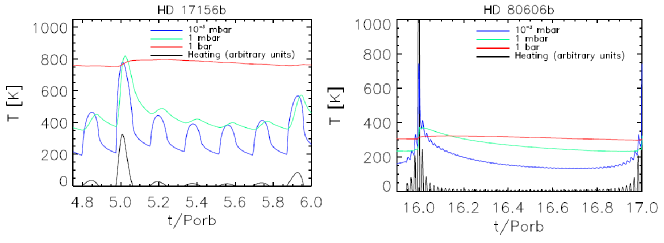
Figure 2.— Temperature of the planet atmospheres, for a single longitude at selected pressure levels (10^-3 mbar, 1 mbar and 1 bar) as a function of time. The heating is a factor that is applied to the incident flux with respect to an averaged incoming flux model ($F_{\star}^{\rm inc}/F_{\star}^{0}$), as defined by Equation 2. We let the calculation make several orbital revolution in order to reach a periodic solution (typically 5 for HD17156b and 16 for HD80606b). Note the different scales in temperature between the two planets.

Figure 3 shows all the thermal structures of one latitude during an orbit. We can see again that deeper than 5 bar, the atmosphere is only weakly dependent on the incoming heating variation. On the other hand, above the 100 mbar level, some of the profiles exhibit a temperature inversion. This inversion is generated by the strong heating by the star when the planet is closer—near periastron. It should be noted that no change of chemistry is taken into account here so the change of irradiation is sufficient for causing this inversion. The inversion reaches an amplitude of $\sim$ 300 K. This inversion has been previously inferred for highly irradiated planets (Burrows et al., 2006; Fortney et al., 2008). Fortney et al. (2008) distinguished two types of planets by the degree of incoming radiation causing or not this inversion (pM class planets experiencing a very high stellar radiation exhibit an inversion whereas cooler pL class planets do not). As we show here, the highly eccentric planets are then likely to transfer from one class to the other during the course of their orbit.

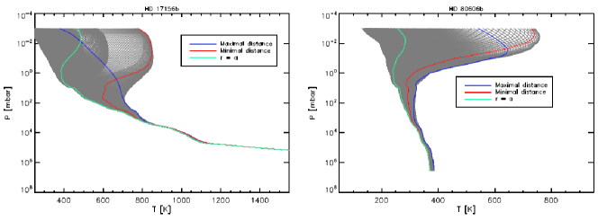
Figure 3.— Temperature structures of the atmospheres for several orbital position (lines) and for each time steps (shaded area). Note the different scales.

Figure 4 represents an equatorial cut of the atmosphere showing the thermal structure as a function of pressure for several phases during an orbit. The rotation leads to a moving of the hottest zone with time. As a consequence of the finite radiative timescale, the hottest zone is shifted with respect to the maximum of insolation (taking place at the substellar point). Moreover, the eccentric orbit generates a global decrease of temperature from the first panel to the fourth as well as a uniformization of the temperature with a lower day to night contrast. During the periastron encounter, the high incoming stellar flux leads to a thermal inversion (as shown in panels 1 and 5) as noted above. Because of the finite radiative timescale, the inversion location is not centered at the substellar point but is delayed in the direction of the rotation of about 10^∘ (non-constant due to the speed difference between the rotation and the heat propagation).

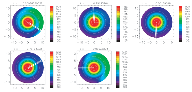
Figure 4.— Thermal structure of the planet HD17156b atmosphere for selected times during the orbit ($t/P_{\rm orb}$ = 0; 0.25; 0.5; 0.75 and 1). The axis represent the pressure in logarithmic scale. The circles from center out indicate the 10³, 1 and 10^-3 bar levels. The substellar point direction is indicated by the black line, fixed at a single location to facilitate comparison between frames. The white line indicates the direction of the Earth. The time is shown as fractions of one orbit. The area contained in the rectangle is the parcel of atmosphere whose temperature evolution is plotted in Figure 2 (in pseudo-synchronous rotation).
An animation of this figure is available in the online journal.

Flux ratio

Figure 5 shows the planet to star flux ratio as a function of wavelength. For the coldest profiles, the features—in absorption—are mainly caused by H₂O and CO. As previously discussed in the models including a thermal inversion (Hubeny et al., 2003; Burrows et al., 2006; Fortney et al., 2008), the features are seen in emission near periastron due to the inversion of temperature.

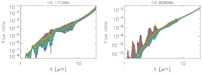
Figure 5.— Ratio of the planet flux by the star flux as a function of wavelength for every times (shaded area) and at several positions (lines).
A color version of this figure is available in the online journal.

Predictions for Spitzer observations

Croll et al. have observed the system during the Cycle 5 of Spitzer with IRAC for 30 hr (pid: 50747). The data have not been published yet.

Figure 6 represents the predicted light curve in the Spitzer 8$\mu$m band. It can be compared to Figure 4 of Irwin et al. (2008). Our results have a smaller amplitude of variation, but we do not account for winds. The flux ratio in our model goes from $\sim 1.3\times 10^{-4}$ to $\sim 4.3\times 10^{-4}$ during the orbit.

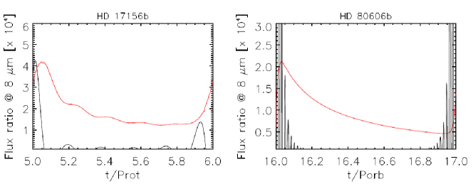
Figure 6.— Evolution of the flux ratio ($\frac{F_{\rm plan.}}{F_{\star}}$) in the Spitzer 8 $\mu$m as a function of time. We integrated the flux emited from the hemisphere seen from Earth; the viewing geometry from the orbit as well as due to the pseudo-synchronous rotation has been taken into account. Note that the scale changes between the two panels.
A color version of this figure is available in the online journal.

3.2.2 HD 80606b

HD 80606b (catalog ) has been discovered by Naef et al. (2001). The high eccentricity of 0.932 leads to a factor $\sim$ 800 of insolation between apastron and periastron.

Previous studies

Langton & Laughlin (2008) performed a hydrodynamic model of this planet. They predicted the planet to star ratio $F_{\rm p}/F_{\star}$ in the 8 $\mu$m band to vary from $\sim 4\times 10^{-4}$ to $\sim 6.5\times 10^{-4}$ from $\sim 20$ hr preceding periastron until $\sim 40$ hr following periastron.

As recently published, Laughlin et al. (2009) observed the secondary eclipse of this planet with Spitzer in the 8 $\mu$m band. The analysis of the light curve is consistent with their predicted radiative time at the 570 mbar level of $\sim$ 4.5hr. Moutou et al. (2009) confirmed that the planet transits its star and analyzed a transit event. They inferred a planetary radius of $R_{\rm pl}=0.86\pm 0.1$ R_J.

Thermal structure

The temperature contrasts from day side to night side are less pronounced than in the case of HD 17156b, due to a globally cooler planet and thus a longer radiative timescale as well as a shorter rotation period of $\sim$ 1.72 days as we can see in Figure 2.

Moreover, as we can see in Figure 3, the planet is globally more isothermal below 10 mbar than in the case of HD 17156b. The temperature difference from 10 mbar to the highest pressures is less than 100 K. On the other hand, above 10 mbar, the temperature inversion—when present—is very large, reaching a 400 K peak. This is due to the fact that although the planet is on average cooler than HD 17156b, its periastron distance ($\sim$ 0.029 AU, almost half of HD 17156b’s) is so short that during the periastron encounter the planet receives a blast of radiation from its star.

Figures 2 and 7 show that the very large planet-star distance variation leads to a greater temperature difference between periastron and apastron. In Figure 7, we can see that the relatively fast rotation cause a large shift between the substellar point and the hottest spot—almost 180^∘ in the first panel but highly varying since the planet rotates faster than the temperature propagation and also the radiative timescale depends on the atmosphere temperature.

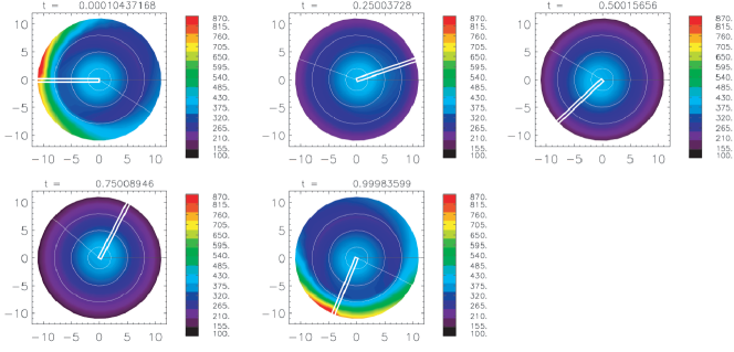
Figure 7.— Same as Figure 4 for the planet HD80606b (with a different temperature scale).
An animation of this figure is available in the online journal.

Our consistent radiative transfer model however, gives temperatures lower than presented by Langton & Laughlin (2008). We reach temperatures up to 900 K, to be compared with the 1200 K obtained by these authors. In comparison, our model cannot represent latitudinal atmospheric flows but it has a consistent vertical structure. Moreover, the long radiative timescale due to the cold temperatures of the planet prevent very large temperature contrasts to occur due to radiative effects alone.

In Figure 5, we can see that the very important temperature inversion leads to emission features that are very large. In contrast, the cold temperatures of the distant apastron lead to absorption features that are a lot fainter.

Predictions for Spitzer observations

In Figure 6, we can see that HD80606b’s light curve is smooth, due to the fast rotation of the planet, but contrary to the hydrodynamic simulations of Langton & Laughlin (2008), we do not achieve a peak of the flux ratio as strong as $8\times 10^{-4}$ but rather $2.1\times 10^{-4}$.

This small amplitude variation does not reproduce Laughlin et al. (2009) observed light curve during secondary eclipse. In this case, the very short but intense heating increase cannot generate the observed planetary flux if we account for radiation effects alone and we have to take into account hydrodynamic processes.

4. Discussion

4.1. Role of the initial inputs to the model

The main limitation of our model is that we do not vary the chemical composition of the atmosphere in lock step with changes in the thermal profile. In order to quantify the error produced by using a constant abundance profile of the constituents, we conducted a test for the planet HD 17156b assuming the two different extreme values for heating and cooling rates, as well as the abundances, calculated for the hottest and coldest profiles obtained by the previous study. Although the calculations take a different amount of time before reaching a periodic solution (the longer radiative timescale for a colder thermal profile makes the model slower to converge), the final periodic solution gives similar results for a complete orbit. Figure 8 shows the relative differences in the final thermal structure as a function of time using the two extremes initial temperature and heating/cooling rates. The largest value is less than 0.5%.

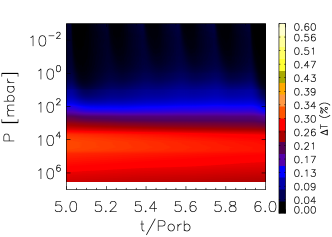
Figure 8.— Relative difference of resulting temperature at each level between the two extremal initial profiles. Profiles using the initial conditions from the hottest and coldest profiles achieved by the nominal calculations for HD17156b have been calculated. Here, the relative differences between the two extreme cases for each pressure level as a function of time are shown.
A color version of this figure is available in the online journal.

This is consistent with the estimation of the calculation time of CO–CH₄ chemical reaction, which is the one determining the main spectral features of the planet. We calculated this reaction time using the prescription of Bézard et al. (2002). For HD17156b, this time above the 250 mbar pressure level—where the temperature variations begin to be relatively important—is less than 10⁷ s, more than the time of the orbit. And the cooler planet HD80606b has even longer chemical timescales $\sim 3\times 10^{15}$ sec. These results justify our approach of not changing the chemical composition with time.

In order to confirm this conclusion, we calculated the flux viewed from Earth integrated in the 8 $\mu$m band for the two extremal initial profiles for HD17156b. This results in little differences, as shown in Figure 9.

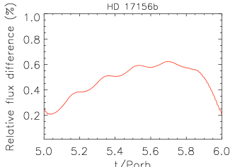
Figure 9.— Relative difference of resulting flux ratio integrated in the 8 $\mu$m band. As in Figure 8, this shows that using the coldest or the hottest profile from the nominal calculations for HD17156b as initial starting point has little effect on the final light curve obtained.

We have adopted solar composition for all our calculations. If we increase the metallicity, we expect the general thermal structure to be slightly hotter due to the higher opacity and thus greater absorption of incoming flux (Fortney et al., 2006). Global spectral features have been shown to exhibit only minor differences due to metallicity in the 8 $\mu$m spectral window (Burrows et al., 2006; Fortney et al., 2010). On the other hand, the radiative time scale is proportional to the atmospheric density (Showman et al., 2008) which increases with metallicity, but this timescale also decreases with temperature (higher metallicity atmospheres are hotter). These two effects should compensate each other to a large extent. Consequently, we expect our qualitative conclusions to be insensitive to metallicity variations, to first order.

4.2. Role of the rotation rate

It should be noted that the formalism of Hut (1981) contains uncertainties in the calculation of the rotation period of the planet. For instance, Ivanov & Papaloizou (2007) using another formalism gave a rotation rate equal to $\sim 1.5$ times the circular orbit angular velocity at periastron $\Omega_{p}$ given by: $\Omega_{p}\sim\sqrt{GM_{\star}\over d_{\rm min}^{3}}$, where $M_{\star}$ is the mass of the parent star. With the parameters of HD 17156b, this gives a rotation period of $P_{\rm spin}^{\rm IP}\sim 2.5$ days.

In order to test the effects of the period of rotation, we used the nominal model for HD 17156b with twice the rotation rate and half the rotation rate given by Equation 3 (resp. $P_{\rm spin}=\frac{1}{2}\times P_{\rm spin}^{\rm Hut}\sim 1.9$ days and $P_{\rm spin}=2\times P_{\rm spin}^{\rm Hut}\sim 7.6$ days) as well as the rotation rate given by Ivanov & Papaloizou (2007) ($P_{\rm spin}=P_{\rm spin}^{\rm IP}\sim 2.5$ days).

Moreover, a more rapid rotation rate can mimic a planet wherein uniform zonal winds occur in addition to the rotating frame.

Figures 10 and 11 show the temperature structure of the planet (equatorial cuts) as a function of time for the two opposite cases. The planet with a rotation rate 2 times faster than our nominal profile is more uniform, as expected. The first and last panels of Figure 11 exhibit temperature contrasts up to 300 K at 1 mbar and as the other panels show there is almost no latitudinal contrast below this pressure level when as the planet to star distance increases. On the other hand, with the slowest rotation rate as shown in Figure 10, the day/night contrasts are more pronounced, with a 500 K day/night contrast at the 1 mbar level near periastron and still a $\sim 50$ K contrast far from periastron.

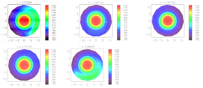
Figure 10.— Same as Figure 4 for $P_{\rm spin}=2\times P_{\rm spin}^{\rm Hut}$ This figure is also available as an mpeg animation in the electronic.
An animation of this figure is available in the online journal.

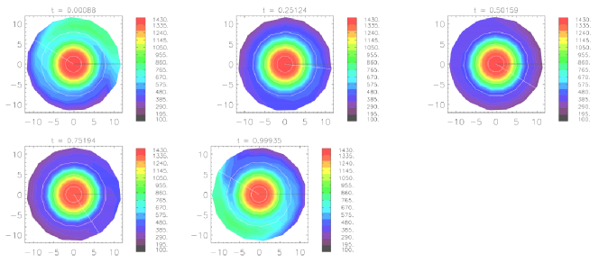
Figure 11.— Same as Figure 4 for $P_{\rm spin}=\frac{1}{2}\times P_{\rm spin}^{\rm Hut}$.
An animation of this figure is available in the online journal.

Figure 12 shows the Spitzer 8$\mu$m light curve for the three cases. The differences are large enough that observations should be able to discriminate between the rotation rate predicted by Hut (1981) or by Ivanov & Papaloizou (2007).

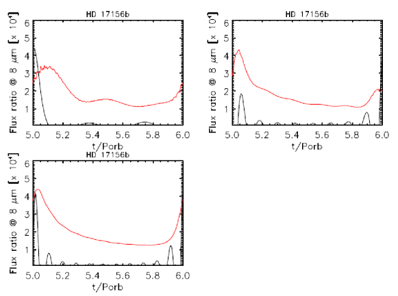
Figure 12.— Same as Figure 6 for $P_{\rm spin}=2\times P_{\rm spin}^{\rm Hut}$ (first panel), $P_{\rm spin}=P_{\rm spin}^{\rm IP}$ (second panel) and $P_{\rm spin}=\frac{1}{2}\times P_{\rm spin}^{\rm Hut}$ (last panel).
A color version of this figure is available in the online journal.

5. Conclusions

We presented a time-dependent radiative model for the atmosphere of the transiting planets. This model takes into account the eccentricity of their orbit as well as the pseudo-synchronous rotation.

We applied our model to the planets HD 80606b and HD 17156b. The results define the radiative portion of the response of these eccentric planets to time-variable stellar insolation and different possible values of the their pseudo-synchronous rotation rate.

We showed that the high eccentricity makes the planets periodically transfer from a state where a stratospheric temperature inversion takes place to a cooler planet with monotonic temperature profiles and vice versa. Significant time variation in an eccentric planet’s spectral features would be expected based on our calculations, and methods to observe such variations phased to the orbit would be very valuable.

Moreover, the maximum of temperature and observable flux is delayed with respect to the maximum of stellar heating (periastrion), due to the finite radiative time

In some cases, an analysis of the planet during the periastron encounter is feasible. It will in principle allow us to discriminate which of the competing theory that predict the pseudo-synchronous rotation period is correct since the temporal variation of the planet flux is relatively highly dependent on its rotation period.

Before reaching a time-dependent radiative model including hydrodynamics, such observations will also help determine if the planet structure is mainly driven by radiation or by atmospheric dynamics.

In the case of HD80606b, the heating increase takes place for a such short time that the radiative model fails to explain the observed flux variation without accounting for hydrodynamic effects.

References

- Bakos et al. (2009) Bakos, G. Á., et al. 2009, arXiv:0901.0282
- Barbieri et al. (2007) Barbieri, M., et al. 2007, A&A, 476, L13
- Bean et al. (2006) Bean, J. L., Benedict, G. F., & Endl, M. 2006, ApJ, 653, L65
- Bézard et al. (2002) Bézard, B., Lellouch, E., Strobel, D., Maillard, J.-P., & Drossart, P. 2002, Icarus, 159, 95
- Burrows et al. (2006) Burrows, A., Sudarsky, D., & Hubeny, I. 2006, ApJ, 650, 1140
- Christian et al. (2009) Christian, D. J., et al. 2009, MNRAS, 392, 1585
- Deming et al. (2007) Deming, D., Harrington, J., Laughlin, G., Seager, S., Navarro, S. B., Bowman, W. C., & Horning, K. 2007, ApJ, 667, L199
- Demory et al. (2007) Demory, B.-O., et al. 2007, A&A, 475, 1125
- Fischer et al. (2007) Fischer, D. A., et al. 2007, ApJ, 669, 1336
- Fortney et al. (2006) Fortney, J. J., Saumon, D., Marley, M. S., Lodders, K., & Freedman, R. S. 2006, ApJ, 642, 495
- Fortney et al. (2008) Fortney, J. J., Lodders, K., Marley, M. S., & Freedman, R. S. 2008, ApJ, 678, 1419
- Fortney et al. (2010) Fortney, J. J., Shabram, M., Showman, A. P., Lian, Y., Freedman, R. S., Marley, M. S., & Lewis, N. K. 2010, ApJ, 709, 1396
- Gillon et al. (2008) Gillon, M., Triaud, A. H. M. J., Mayor, M., Queloz, D., Udry, S., & North, P. 2008, A&A, 485, 871
- Gillon et al. (2009) Gillon, M., et al. 2009, arXiv:0901.4705
- Grillmair et al. (2007) Grillmair, C. J., Charbonneau, D., Burrows, A., Armus, L., Stauffer, J., Meadows, V., Van Cleve, J., & Levine, D. 2007, ApJ, 658, L115
- Hebb et al. (2009) Hebb, L., et al. 2009, ApJ, 693, 1920
- Hubeny et al. (2003) Hubeny, I., Burrows, A., & Sudarsky, D. 2003, ApJ, 594, 1011
- Hut (1981) Hut, P. 1981, A&A, 99, 126
- Iro et al. (2005) Iro, N., Bézard, B., & Guillot, T. 2005, A&A, 436, 719
- Irwin et al. (2008) Irwin, J., et al. 2008, ApJ, 681, 636
- Ivanov & Papaloizou (2007) Ivanov, P. B., & Papaloizou, . C. B. 2007, MNRAS, 376, 682
- Johnson et al. (2008) Johnson, J. A., et al. 2008, ApJ, 686, 649
- Joshi et al. (2009) Joshi, Y. C., et al. 2009, MNRAS, 392, 1532
- Knutson et al. (2007) Knutson, H. A., et al. 2007, Nature, 447, 183
- Langton & Laughlin (2007) Langton, J., & Laughlin, G. 2007, ApJ, 657, L113
- Langton & Laughlin (2008) Langton, J., & Laughlin, G. 2008, ApJ, 674, 1106
- Laughlin et al. (2005) Laughlin, G., Marcy, G. W., Vogt, S. S., Fischer, D. A., & Butler, R. P. 2005, ApJ, 629, L121
- Laughlin et al. (2009) Laughlin, G., Deming, D., Langton, J., Kasen, D., Vogt, S., Butler, P., Rivera, E., & Meschiari, S. 2009, Nature, 457, 562
- Loeillet et al. (2008) Loeillet, B., et al. 2008, aap, 481, 529
- Maness et al. (2007) Maness, H. L., Marcy, G. W., Ford, E. B., Hauschildt, P. H., Shreve, A. T., Basri, G. B., Butler, R. P., & Vogt, S. S. 2007, PASP, 119, 90
- Moutou et al. (2009) Moutou, C., et al. 2009, A&A, 498, L5
- Naef et al. (2001) Naef, D., et al. 2001, A&A, 375, L27
- Showman et al. (2008) Showman, A. P., Cooper, C. S., Fortney, J. J., & Marley, M. S. 2008, ApJ, 682, 559
- Swain et al. (2008) Swain, M. R., Bouwman, J., Akeson, R. L., Lawler, S., & Beichman, C. A. 2008, ApJ, 674, 482
- Winn et al. (2008) Winn, J. N., et al. 2008, ApJ, 683, 1076