Efficient Evaluation of Casimir Force in Arbitrary Three-dimensional Geometries by Integral Equation Methods

Abstract

In this paper, we generalized the surface integral equation method for the evaluation of Casimir force in arbitrary three-dimensional geometries. Similar to the two-dimensional case, the evaluation of the mean Maxwell stress tensor is cast into solving a series of three-dimensional scattering problems. The formulation and solution of the three-dimensional scattering problem is well-studied in classical computational electromagnetics. This paper demonstrates that this quantum electrodynamic phenomena can be studied using the knowledge and techniques of classical electrodynamics.

The Casimir force has first been predicted by Casimir in 1948 Casimir_1948 . It exists among charge-neutral bodies due to the quantum fluctuation of the elecromagnetic fields in vacuum. Although it is tiny when the objects have large separations, it becomes the dominant force between charge-neutral objects when the separation is below micron meters.

Micro-electromechanical systems (MEMS) are micron-sized devices in which mechanical elements and moving parts, such as tiny sensors and actuators are carved into a silicon substrate. As further miniaturization takes place, the devices may reduce to nano-scale and become nanoelectromechanical systems (NEMS). They have a wide class of applications. For example, the release of the airbag in cars is controlled by a MEMS-based accelerometer. One of the principal causes of malfunctioning in MEMS is stiction, i.e., the collapse of movable elements into nearby surfaces, resulting in their permanent adhesion. Casimir effect is often an important underlying mechanism causing this phenomenon Buks_2001 . On the other hand, this effect could be put into good use. Capasso and his group showed that the force can be used to control the actuation of a micromachined torsional device Chan_2001sci . This group also showed that the Casimir attraction can be used to make a nonlinear oscillator. The force influences the dynamical properties of a micromachined device, changing its resonance frequency, hysteretic behavior, and bistability in its frequency response to an AC excitation. They proposed that this device could serve as a position sensor working in nanometer scale Chan_2001prl ; Capasso_munday_2007 .

Since Casimir effect is rather significant in MEMS and NEMS devices, it is important to be able to predict it accurately before the devices going into manufacturing. The geometry of the MEMS and NEMS devices may be complicated; thus approximation methods, such as the proximity force approximation (PFA) Bordag_2001 , and optical approach in terms of virtual photons moving along ray optical paths Scardicchio_2005 , are no longer sufficient. Instead, an exact and general numerical method that can handle arbitrary geometry is desired. With the numerical method, we can get the desired accuracy by giving enough computational resource. Recently, major progress has been made in the development of numerical methods for Casimir force. In general, there are two popular approaches: the path integral approach (also known as EGJK method) and the Maxwell stress-tensor approach.

Schwinger is the first one to attribute the Casimir interaction to fluctuating current and charge densities inside the objects. With path integral method, the Casimir energy is expressed as the logarithm of a functional integral over all allowed configurations of the fluctuating currents, weighted by the appropriate action Buscher_2005 . It has been generalized in EGJK_2007 (EGJK) for compact objects of arbitrary shape and separation and applied to predict the force between a cylinder and a plate Emig_2006 , and between two spheres EGJK_2007 . EGJK’s agorithm is efficient to predict the Casimir energy between compact 3D objects of spheroidal or nearly-spheroidal shape. The algorithm leads to analytically tractable series solution. But it is not of practical use for general geometries due to the poor convergence rate for objects with corners. This limitation occurs since they used spherical basis functions to expand the current distribution. It could be overcome by expanding the currents with basis functions defined on a pair of adjacent triangles, which is known as the RWG basis Reid_2009 ; RWG . The RWG basis is vastly popular in the surface integral method in computational electromagnetics. After some manipulation, the evaluation of Casimir energy depends only on solving for all the eigenvalues of the impedance matrix obtained from the integral equation by the method of moments.

The theoretical foundation for the Maxwell stress tensor approach was built by Lifshitz and his coworkers dzyaloshinskii_1961 : the net Casimir force on a body can be expressed as an integral over any closed surface around the body of the mean electromagnetic stress tensor, integrated over all frequencies. And the fluctuation-dissipation theorem states that the mean fluctuating field, which forms the Maxwell stress tensor, is related to the imaginary part of the dyadic Green’s function of the same geometry. The dyadic Green’s function can be evaluated by existing numerical methods in computational electromagnetics (electrodynamics) Rodriguez_2007pra . Rodriguez has demonstrated the applicability of this method by using a simple finite-difference frequency-domain (FDFD) method to calculate the dyadic Green’s function in $z$-invariant structures Rodriguez_2007prl ; Rodriguez_2008 . This approach relates the quantum electrodynamic phenomena with classical electromagnetics which motivates our piece of work: to evaluate the Casimir force among arbitrary objects using integral equation method. With surface integral equation method, the number of unknowns can be greatly reduced. Moreover, fast algorithms book_chew_2001 are available to further improve the efficiency of the method. The computational complexity of both the stress tensor approach and the path integral approach can be reduced to $O(N\log N)$ times the number of iterations at best, $N$ being the number of surface unknowns. Thus their efficiency is comparable. The main difference between them is the physical quantity being calculated directly: path integral method calculates the energy while stress tensor approach calculates the force distribution (pressure).

In a paper published earlier Jie_2009 , we have demonstrated that surface integral equation method could be applied to evaluate the dyadic Green’s function and its derivatives in two-dimensional (2D) geometries. By using this method, the Casimir force between 2D objects could be simulated using much fewer unknowns and can be easily accelerated by fast-algorithms readily developed in computational electromagnetics. In this paper, we would extend the surface integral equation method for arbitrary three-dimensional (3D) geometries. The idea is similar to the last paper Jie_2009 : the Casimir force is expressed in terms of the dyadic Green’s function and its derivatives and they could be calculated from the integral equation by using different types of dipole point sources.

The starting point of the stress tensor approach is that the net Casimir force acting on the surface $S$ of an object is given by an surface integral of the mean stress tensor on it Rodriguez_2007pra :

$$\mbox{${\bf F}$}=\oint_{S}\langle\mbox{$\overline{{{\bf T}}}$}({{\bf r}}^{\prime})\rangle\cdot d{{\bf s}}^{\prime}$$ (1)

where $\overline{{{\bf T}}}$ is the Maxwell stress tensor defined as in jackson_1975 . For an arbitrary 3D object, we define $\hat{u}$ and $\hat{v}$ as the tangent vector at the surface, and $\hat{n}$ as the normal direction of the surface. They satisfy the relationship $\hat{u}\times\hat{v}=\hat{n}$. If the object is a perfect conductor, the tangential electric field $E_{u}$, $E_{v}$ and the normal magnetic field $B_{n}$ vanishes at the surface of the object. The stress tensor could be simplified as follows:

$$T_{nn}({{\bf r}}) = \frac{1}{2}\epsilon_{0}E^{2}_{n}({{\bf r}})-\frac{1}{2\mu_{0}}B^{2}_{u}({{\bf r}})-\frac{1}{2\mu_{0}}B^{2}_{v}({{\bf r}})$$ (2)

$$T_{un}({{\bf r}}) = T_{vn}({{\bf r}})=0$$ (3)

Thus for perfect conductors, the Casimir force becomes a pressure on the surface.

The average of the fluctuating electric and magnetic fields in the ground state is obtained from the fluctuation-dissipation theorem landau_1980 :

$$\langle 0|\hat{E}_{i}({{\bf r}},t)\hat{E}_{j}({{\bf r}}^{\prime},t)|0\rangle = \frac{\hbar}{\pi}\text{Im}\int_{0}^{\infty}\omega^{2}{G}_{ij}({{\bf r}},{{\bf r}}^{\prime},\omega)d\omega$$ (4)

$$\langle 0|\hat{B}_{i}({{\bf r}},t)\hat{B}_{j}({{\bf r}}^{\prime},t)|0\rangle = \frac{\hbar}{\pi}\text{Im}\int_{0}^{\infty}(\nabla\times)_{il}(\nabla^{\prime}\times)_{jm}G_{lm}({{\bf r}},{{\bf r}}^{\prime},\omega)d\omega$$ (5)

where the dyadic Green’s function is the same as that defined in classical electromagnetics to relate the current to the field in an arbitrary geometry Jie_2009 .

In 3D structures, the field components and the dyadic Green’s function satisfy the following relationship:

$$E_{\alpha}({{\bf r}}) = i\omega\int_{S}d{{\bf r}}^{\prime}{G}_{\alpha\beta}(k,{{\bf r}},{{\bf r}}^{\prime}){J}_{\beta}({{\bf r}}^{\prime})$$ (6)

$$H_{u}({{\bf r}}) = \frac{1}{\mu_{0}}\int_{S}d{{\bf r}}^{\prime}\left[\frac{\partial}{\partial v}G_{n\beta}(k,{{\bf r}},{{\bf r}}^{\prime})-\frac{\partial}{\partial n}G_{v\beta}(k,{{\bf r}},{{\bf r}}^{\prime})\right]{J}_{\beta}({{\bf r}}^{\prime})$$ (7)

Substituting (6) and (7) into (4) and (5), the average of each term in the stress tensor could be represented by

$$\frac{1}{2}\epsilon_{0}\langle E_{n}({{\bf r}})E_{n}({{\bf r}}^{\prime})\rangle = \frac{\hbar c_{0}}{2\pi\mu_{0}}\text{Im}\int_{0}^{\infty}\frac{k^{2}_{0}}{i\omega}E_{n}(k_{0},{{\bf r}},s_{1})dk_{0}$$ (8)

$$\frac{1}{2\mu_{0}}\langle B_{u}({{\bf r}})B_{u}({{\bf r}}^{\prime})\rangle = \frac{\hbar c_{0}}{2\pi}\text{Im}\int_{0}^{\infty}dk_{0}\left[-H_{u}(k_{0},{{\bf r}},s_{2})+H_{u}(k_{0},{{\bf r}},s_{3})\right]$$ (9)

$$\frac{1}{2\mu_{0}}\langle B_{v}({{\bf r}})B_{v}({{\bf r}}^{\prime})\rangle = \frac{\hbar c_{0}}{2\pi}\text{Im}\int_{0}^{\infty}dk_{0}\left[-H_{v}(k_{0},{{\bf r}},s_{4})+H_{u}(k_{0},{{\bf r}},s_{5})\right]$$ (10)

Here, ${{\bf E}}(k_{0},{{\bf r}},s_{i})$ and ${{\bf H}}(k_{0},{{\bf r}},s_{i})$ are the electric/magnetic field at location ${{\bf r}}$ in the geometry under the excitation of source $s_{i}$. Their corresponding relationships are summarized in Table 1.

Table 1: A table of source and field operators for each term in the stress tensor.

	Field Component	Source   $({{\bf r}}_{i}={{\bf r}})$
(1)	$E_{n}({{\bf r}},s_{1})$	$\hat{n}{\delta}({{\bf r}}^{\prime}-{{\bf r}}_{i})$
(2)	$H_{u}({{\bf r}},s_{2})$	$\hat{v}\ \frac{\partial}{\partial n^{\prime}}{\delta}({{\bf r}}^{\prime}-{{\bf r}}_{i})$
(3)	$H_{u}({{\bf r}},s_{3})$	$\hat{n}\ \frac{\partial}{\partial v^{\prime}}{\delta}({{\bf r}}^{\prime}-{{\bf r}}_{i})$
(4)	$H_{v}({{\bf r}},s_{4})$	$\hat{n}\ \frac{\partial}{\partial u^{\prime}}{\delta}({{\bf r}}^{\prime}-{{\bf r}}_{i})$
(5)	$H_{v}({{\bf r}},s_{5})$	$\hat{u}\ \frac{\partial}{\partial n^{\prime}}{\delta}({{\bf r}}^{\prime}-{{\bf r}}_{i})$

If the object is made of perfect conducting material, there is only induced electric current ${{\bf J}}$ flowing on the surface. The scattered electric field and magnetic field in the free space region could be obtained from the induced electric current by $\mathcal{L}$ and $\mathcal{K}$ operators respectively PMCHWT :

$${{\bf E}}({{\bf r}}) = {{\bf E}}^{i}({{\bf r}})+\mathcal{L}{{\bf J}}({{\bf r}})$$ (11)

$${{\bf H}}({{\bf r}}) = {{\bf H}}^{i}({{\bf r}})-\mathcal{K}{{\bf J}}({{\bf r}})$$ (12)

where ${{\bf E}}$ and ${{\bf H}}$ are the total field in the space and ${{\bf E}}^{i}$ and ${{\bf H}}^{i}$ are the incident field generated by an external source. The operators are defined as

$$\mathcal{L}{{\bf X}}({{\bf r}}) = i\omega\mu_{0}\int_{s}\left[\mbox{$\overline{{{\bf I}}}$}+\frac{\nabla\nabla}{k^{2}_{0}}\right]g({{\bf r}},{{\bf r^{\prime}}})\cdot{{\bf X}}({{\bf r^{\prime}}})d{{\bf r^{\prime}}}$$ (13)

$$\mathcal{K}{{\bf X}}({{\bf r}}) = \int_{s}{{\bf X}}({{\bf r^{\prime}}})\times\nabla g({{\bf r}},{{\bf r^{\prime}}})d{{\bf r^{\prime}}}$$ (14)

where $g({{\bf r}},{{\bf r}}^{\prime})=e^{ik_{0}|{{\bf r}}-{{\bf r}}^{\prime}|}/4\pi|{{\bf r}}-{{\bf r}}^{\prime}|$. The total tangential electric field vanishes on the surface of the PEC object. Enforcing Eqn. (13) on the surface we obtain the electric field integral equation(EFIE):

$$-\hat{n}\times{{\bf E}}^{i}({{\bf r}})=\hat{n}\times\mathcal{L}{{\bf J}}({{\bf r}})$$ (15)

By expanding the unknown current with RWG basis RWG , ${{\bf J}}({{\bf r}}^{\prime})=\sum_{n}a_{n}{{\bf J}}_{n}({{\bf r}}^{\prime})$ and using Galerkin’s method, the integral equation (15) could be cast into a matrix equation $[Z_{mn}][a_{n}]=[g_{m}]$, where

$$g_{m} = \int_{T_{m}}d{{\bf r}}{{\bf J}}_{m}({{\bf r}})\cdot{{\bf E}}^{i}({{\bf r}})$$ (16)

$$Z_{mn} = i\omega\mu_{0}\int_{T_{m}}d{{\bf r}}\int_{T_{n}}d{{\bf r}}^{\prime}{{\bf J}}_{m}\cdot\left[\mbox{$\overline{{{\bf I}}}$}+\frac{\nabla\nabla}{k^{2}_{0}}\right]g({{\bf r}},{{\bf r}}^{\prime})\cdot{{\bf J}}_{n}({{\bf r}}^{\prime})$$ (17)

If the sources listed in Table 1 are used to generate the incident field, then the evaluation of $g_{m}$ involves integrals containing some super-hyper singularities. The treatment of these singularities has been discussed in detail in Meisong_2007 .

Now we would present some numerical results obtained from this method. They are compared with either analytical results or other’s calculation. First we would start with the evaluation of the Casimir force between two spheres, since they are the simplest 3D objects and the analytical expression of the Casimir energy is available in EGJK_2007 . We assume that the radius of both spheres is $R$ and their minimum distance is $Z$, the product of the force and the square of the radius ($F*R^{2}/\hbar c_{0}$) is a dimensionless and scale-invariant quantity. So the result is given by their product ($F*R^{2}/\hbar c_{0}$) versus the normalized separation ($Z/R$). In the numerical process, first the Casimir force per unit area (pressure) is calculated at different points on the surface, and then the total force is obtained by integrating the pressure over the entire surface. The analytical results are interpolated from the data given in ref. EGJK_2007 . Good agreement has been observed.

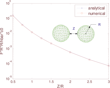
Figure 1: Casimir force between two spheres of radius $R$ and a separation of $Z$.

The geometry of the second example contains two identical capsules. A capsule is a cylinder of radius $R$ with hemispherical end caps. Its total length is denoted by $L$. Experiment had been carried out to measure the interaction between two crossed cylindrical capsules Ederth_2000 so a numerical study of the geometry would be interesting to experimentalist. It has also been simulated by using EGJK method in ref. Reid_2009 and reference data is available to make comparison. The force between two capsules is evaluated for two cases: they are parallel or they are perpendicular.

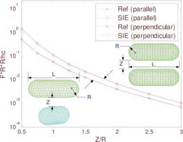
Figure 2: Casimir for two pairs of perfectly conducting objects: identical capsules with parallel axes, and identical capsules with perpendicular axes. Here $L=6R$. SIE refers to the surface integral equation method derived in this paper.

Similar to the 2D geometries Jie_2009 case, the integral equation method could reduced the computation cost significantly since it involves only surface unknowns. Moreover, both the coordinate space integration (1) and the spectral space integration (8) to (10) are smooth and independent of the number of unknowns.

As we know, both our surface integral method following the stress tensor approach and Reid et al numerical method following the path integral approach Reid_2009 are effective numerical methods for calculating the Casimir force among arbitrary 3D objects. Though they start from completely different description of the Casimir energy and force, they are connected with the surface integral equation method in classical electromagnetics at certain stage. Reid et al method reduces the problem to a search of the all eigenvalues of the impedance matrix. Our method reduces the problem to solving a set of matrix equation, with the same impedance matrix as in Reid et al method. Reid et al method calculates energy directly while our method calculates the force distribution directly. The complexity of both method could be reduced to $O(N\log N)$ at best by using fast algorithms, where $N$ is the number of surface unknowns. The drawback of the path integral method is that we need to differentiate the total energy with respect to displacement in a certain direction to get the force. This operation changes the problem into a generalized eigenvalue problem which increases the cost and complexity. Another drawback is that the force distribution on the surface is not available from the method. On the contrary, for stress tensor approach, force distribution is required before we obtain the total force. The tradeoff is that an additional surface integral needs to be performed compared to the path integral method.

References

- (1) H. B. G. Casimir, Proc. K. Ned. Akad. Wetensch. 51, 793 (1948).
- (2) E. Buks and M. L. Roukes, Phys. Rev. B 63, 033402(2001).
- (3) H. B. Chan, V. A. Aksyuk, R. N. Kleiman, D. J. Bishop, and F. Capasso, Science 291, 1941 (2001).
- (4) H. B. Chan, V. A. Aksyuk, R. N. Kleiman, D. J. Bishop, and F. Capasso, Phys. Rev. Lett. 87, 211801 (2001).
- (5) F. Capasso, J. N. Munday, D. Iannuzzi and H. B. Chan, Selected Topics in Quantum Electronics, IEEE Journal of 13, 400 (2007).
- (6) M. Bordag, U. Mohideen and V. M. Mostepanenko, Phys. Rep. 353, 1 (2001).
- (7) A. Scardicchio and R.L. Jaffe, Nucl. Phys. B, 704 (2005).
- (8) R. Büscher and T. Emig, Phys. Rev. Lett. 94, 133901(2005)
- (9) T. Emig, N. Graham, R. L. Jaffe and M. Kardar, Phys. Rev. Lett. 99, 170403 (2007).
- (10) T. Emig, R. L. Jaffe, M. Kardar and A. Scardicchio, Phys. Rev. Lett. 96, 080403 (2006).
- (11) M. T. Homer Reid, A. W. Rodriguez, J. White, S. G. Johnson, Phys. Rev. Lett. 103, 040401(2009)
- (12) S. M. Rao, D. R. Wilton and A. W. Glisson, IEEE Trans. Antennas Propagat. 30, 409 (1982).
- (13) I. E. Dzyaloshinskii, E. M. Lifshitz and L. P. Pitaevskii, Physics-Uspekhi 4, 153 (1961).
- (14) A. W. Rodriguez, M. Ibanescu, D. Iannuzzi, J. D. Joannopoulos, and S. G. Johnson, Phys. Rev. A 76, 032106 (2007).
- (15) A. W. Rodriguez, M. Ibanescu, D. Iannuzzi, F. Capasso, J. D. Joannopoulos and S. G. Johnson, Phys. Rev. Lett. 99, 080401(2007).
- (16) A. W. Rodriguez, J. D. Joannopoulos and S. G. Johnson, Phys. Rev. A 77, 062107 (2008).
- (17) W. C. Chew, J. M. Jin, E. Michielssen, J. M. Song, Fast and Efficient Algorithms in Computational Electromagnetics, (Artech, Norwood, MA, 2001).
- (18) J. D. Jackson, Classical Electrodynamics ,3rd ed. (Wiley, New York, 1998).
- (19) L. D. Landau, E.M. Lifshitz and L. P. Pitaevskii, Statistical physics. Part 2, (Pergamon Press, 1980).
- (20) J. L. Xiong and W. C. Chew, Appl. Phys. Lett. 95, 154102 (2009).
- (21) L. N. Medgyesi-Mitschang, J. M. Putman and M. B. Gedera, J. Opt. Soc. Am. A 11, 1383 (1994).
- (22) M. S. Tong and W. C. Chew, Microwave Opt. Technol. Lett. 49, 1383 (2007).
- (23) T. Ederth, Phys. Rev. A 62, 062104 (2000).