A Far-UV Survey of M 80: X-ray Source Counterparts, Strange Blue Stragglers and the Recovery of Nova T Sco.

Abstract

Using the ACS on HST, we have surveyed the $FUV$ and $NUV$ populations in the core region of M 80. The CMD reveals large numbers of blue and extreme horizontal branch stars and blue stragglers, as well as $\approx 60$ objects lying in the region of the CMD where accreting and detached white dwarf binaries are expected. Overall, the blue straggler stars are the most centrally concentrated population, with their radial distribution suggesting a typical blue straggler mass of about $1.2~{}M_{\odot}$. However, counterintuitively, the faint blue stragglers are significantly more centrally concentrated than the bright ones and a Kolmogorov-Smirnov test suggest only a 3.5% probability that both faint and bright blue stragglers are drawn from the same distribution. This may suggest that (some) blue stragglers get a kick during their formation. We have also been able to identify the majority of the known X-ray sources in the core with $FUV$ bright stars. One of these $FUV$ sources is a likely dwarf nova that was in eruption at the time of the $FUV$ observations. This object is located at a position consistent with Nova 1860 AD, or T Scorpii. Based on its position, X-ray and UV characteristics, this system is almost certainly the source of the nova explosion. The radial distribution of the X-ray sources and of the cataclysmic variable candidates in our sample suggest masses $>1M_{\odot}$.

1 Introduction

Far-UV ($FUV$) observations are an ideal tool to study the exotic stellar populations that reside in globular clusters (GCs), such as blue stragglers (BSs), white dwarfs (WDs), cataclysmic variables (CVs, binaries containing an accreting WD), low-mass X-ray binaries (LMXBs, binaries containing an accreting neutron star or black hole), blue and extreme horizontal branch (BHB and EHB) stars, and blue hook (BHk) stars. Identifying these exotica in visible light can be extremely difficult, partly due to the severe crowding of optical images (especially of the cores of GCs) which are dominated by main sequence (MS) stars and red giants (RGs), and partly because most exotica are optically faint. However, all of these exotic populations tend to be hotter than other cluster members and emit much of their radiation in the $FUV$. “Ordinary” cluster stars (MS stars and RGs) are cooler and considerably fainter at wavelengths less than 2000 Å. As a result, crowding is generally not a problem in the $FUV$. Thus, deep $FUV$-imaging at high spatial resolution with $HST$ is an excellent way to detect and study exotic stellar species.

So far, deep $FUV$ studies have been carried out for only three clusters: 47 Tuc (Knigge et al. 2002, 2003, 2008), NGC 2808 (Brown et al. 2001, Dieball et al. 2005a, Servillat et al. 2008), and M 15 (Dieball et al. 2005b, 2007). In 47 Tuc, Knigge et al. (2002) found $FUV$ counterparts for the four Chandra CV candidates (Grindlay et al. 2001) known at that time within the $FUV$ field of view. All of these were found to be variable $FUV$ excess sources and three of them were later spectroscopically confirmed as CVs (Knigge et al. 2008). In NGC 2808, Brown et al. (2001) used $FUV$ and $NUV$ imaging to uncover a population of sub-luminous hot horizontal branch (HB) stars, the BHk stars, and suggested that this population is the result of a late helium-core flash on the WD cooling curve. Dieball et al. (2005a) re-analyzed the $HST$ data on NGC 2808 and found numerous BSs, CV candidates and hot young WDs. Servillat et al. (2008) found 8 $FUV$ counterparts to the Chandra X-ray sources in the core of NGC 2808; two of those are close matches and confirm their CV nature. In M 15, Dieball et al. (2005b) found the $FUV$ counterpart of the LMXB M 15 X-2 (White & Angelini 2001), and clearly detected an orbital period of 22.6 minutes, thus confirming M 15 X-2 as an ultracompact X-ray binary (UCXB), only the third in a GC at that time. Since then, Zurek et al. (2009) have confirmed the UCXB status of another X-ray source in the GC NGC 1851, also based on FUV observations. Dieball et al. (2007) constructed a deep $FUV-NUV$ color magnitude diagram (CMD) for M 15, which revealed large numbers of CV and WD candidates, a well defined BS and HB sequence, and 41 variable $FUV$ sources, amongst them RR Lyrae, Cepheids, SX Phoenicis stars, CVs, and the well known LMXB AC 211.

Here we present the results of $FUV$ and $NUV$ imaging observations with the Advanced Camera for Surveys (ACS) with the $Hubble~{}Space~{}Telescope~{}(HST)$ of the GC M 80. This cluster is one of the densest in the Galaxy and has a metallicity of $[\rm{Fe/H}]=-1.7$ dex (Brocato et al. 1998, Alcaino et al. 1998, Cavallo et al. 2004), a distance of 10 kpc, and a reddening of $E_{B-V}=0.18$ mag (Harris 1996). Despite being a very dense and compact cluster ($r_{core}=9\arcsec$ corresponding to 0.44 pc at 10 kpc, $r_{halfmass}=39\arcsec$ corresponding to 1.89 pc, Harris 1996), M 80 is not thought to be a core-collapsed cluster. Ferraro et al. (1999, 2003) found a large and centrally concentrated population of BSs, and suggested that M 80 is in a state in which core-collapse is delayed by the production of an extraordinarily large population of collisional BSs. Only a few variable sources are known in M 80 (Wehlau et al. 1990, Clement & Walker 1991, Clement et al. 2001). Based on the periods of the six RR Lyrae known in this cluster, M 80 is classified as Oosterhoff type II (Oosterhoff 1939).

M 80 is also famous for its historic classical nova T Scorpii, which was discovered in 1860 by Auwers when it outshone the entire cluster (Luther 1860, Pogson 1860). Shara & Drissen (1995) found a very blue star $5\arcsec$ from the cluster center and within $1\arcsec$ of their estimated position for the nova, and thus identified it as the (now quiescent) counterpart of the nova. Our observations, discussed in Section 4, suggest a different candidate. Apart from the nova, two new erupting dwarf novae (DNe) were identified by Shara & Drissen (1995). Based on a 50 ksec of Chandra observations, Heinke et al. (2003) found 19 X-ray sources within the cluster’s halfmass radius to a limiting $L_{\rm{0.5-2.5\,keV}}\approx 7\times 10^{30}\ \rm{erg}\ \rm{s}^{-1}$. They suggested that two of those were quiescent LMXBs and five others were CVs based on their X-ray hardness ratio, and that the brightest source detected might be the X-ray counterpart to the classical nova T Sco.

Our report is structured as follows: In Sect. 2, we describe the observations and the data reduction. In Sect. 3, the analysis of the $FUV-NUV$ CMD is presented. In Sect. 4, we describe our comparison of X-ray to $FUV$ locations and our identification of the quiescent nova with an object which appears to have been undergoing a dwarf nova outburst at the time of our $FUV$ observations. In Sect. 5, we present the radial distribution of the various populations and compare them to the X-ray source distribution. Finally, we summarize our results in Sect. 6.

2 Observations and the Creation of the Catalog

The observations of the core of M 80 were carried out with the ACS onboard HST using the $FUV$ F165lp filter in the Solar Blind Channel (SBC) and the $NUV$ F250W filter in the High Resolution Channel (HRC) and were made at a single pointing position. The SBC has a field of view of $35\arcsec\times 31\arcsec$ with a pixel size of $0\farcs 034\times 0\farcs 030$, whereas the HRC field of view is slightly smaller with $29\arcsec\times 26\arcsec$ and a spatial resolution of $0\farcs 028\times 0\farcs 025$ pixels. Thus, the observations cover only the central portions (approximately 1.5 core radii if we adopt a core radius of $9\arcsec$, Harris 1996) of M 80. The $FUV$ observation was carried out during four consecutive orbits in September 2004. To facilitate searches for time variability, the $FUV$ observation (dataset j8y501) comprised 32 individual exposures of durations ranging from 310-323 seconds. The total exposure time was 10232 sec. The $NUV$ observation (dataset j8y504) comprised a single orbit in October 2004, and resulted in a total exposure of 2384 sec, split into 8 individual exposures of 298 sec. Dithers were not utilized to simplify searches for time variability.

Beginning with the data products delivered by STScI, we created master images of the $FUV$ and $NUV$ data using multidrizzle running under PyRAF. The multidrizzle routines correct the field distortion that exists in the individual flatfielded images delivered as part of the standard data products and combine them into master images for the $FUV$ and $NUV$. The combined and geometrically corrected output master images have a pixel scale of $0.025\arcsec/{\rm pixel}$ and are normalized to 1 sec exposure time.

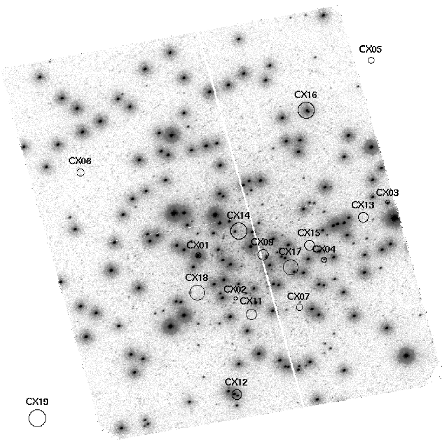
Figure 1: Combined and geometrically corrected master image of all $FUV$ SBC/F165LP exposures taken from M 80’s core region. North is up and east to the left. The field of view is $35\arcsec\times 31\arcsec$. The image is displayed on a logarithmic intensity scale in order to bring out the fainter sources. The positions of the X-ray sources found by Heinke et al. (2003) are marked with their 3$\sigma$ error circles.

The $FUV$ and $NUV$ master images are shown in Fig. 1 and 2. As expected, the $FUV$ image is considerably less crowded than the $NUV$ image. Both images show significant concentrations of sources towards the cluster core.

2.1 $FUV$ and $NUV$ Source Detection

We used daofind (Stetson 1991) running under IRAF to create initial source lists for the $FUV$ and $NUV$ master images. We then checked and updated these lists, adding a few faint stars that were missed by daofind and removing obvious false detections (e.g. multiple detections of very bright sources, noise peaks near image edges, etc.). For a detailed description of the source finding procedure see Dieball et al. (2007). The resulting final catalogs contained 3168 $FUV$ and 9875 $NUV$ sources.

2.2 Matching $FUV$, $NUV$ and Optical Sources

In order to match the $FUV$ and $NUV$ catalogs, we created a reference list containing the pixel coordinates of 92 stars that are clearly visible and well within the fields of both images. We used the geomap and geoxytran task running under IRAF to determine the geometrical transformation between the two catalogs. We allowed for x and y shifts, rotation and scale changes in the coordinate transformation. The residual errors in the transformation were quite small, less than 0.2 pixels ($<$ 10 mas) (RMS) for the 92 stars.

The $FUV$ field is slightly larger than the $NUV$ field and 2574 $FUV$ sources are located within the $NUV$ field of view. After some testing, we adopted a maximum matching tolerance of 2.5 pixels between the $FUV$ and $NUV$ source positions, resulting in 2345 matches (91% of the possible $FUV$ sources). Following the procedure described by Knigge et al. (2002), which is based both on the number of sources which are matched and those which are not matched, we can expect 45 ($\approx 1.9\%$) false matches among these 2345 pairs (but note that this estimate does not account for the increased source concentration towards the core).

We also used the Piotto et al. (2002) catalog of M 80 to search for optical counterparts to our $FUV$ sources. The optical data were obtained using the WFPC2 in 1996, with the PC centered on the cluster center. As a first step, our $FUV$ image coordinate system had to be transformed to the PC image system. For that purpose, we used 31 HB stars as reference objects that could be easily identified in both the PC F555W and the SBC F165LP master image. (Note that five out of these 31 stars are not located within the somewhat smaller field of view of the HRC F250W exposures.) We allowed for a maximum matching tolerance of 1.1 PC pixels (corresponding to $\approx 2$ pixels on our $FUV$ or $NUV$ master images) and found a total of 1418 optical matches to the $FUV$ sources; out of these 1268 are inside the $NUV$ field of view. We can expect $\approx 40$ to be false matches.

2.3 Improving the Absolute Astrometry

Even though multidrizzle corrects the field distortion of our images, it does not improve their absolute astrometric accuracy. The world coordinate system (WCS) of the images provided with the standard data products is based on the original guide star catalog (GSC1), whose absolute positions are often only accurate to $1\arcsec-2\arcsec$. This makes matching to external (e.g. X-ray) catalogs difficult.

The usual way to improve the astrometry in HST images is to locate one or more stars in an image whose positions are accurately known in a Tycho-based system, and to update the astrometric solution of the image. However, because the core of M 80 is so crowded and because the SBC covers such a small region of the sky, we were unable to find appropriate stars in the master images. We therefore adopted a bootstrap approach beginning with an ACS Wide Field Camera (WFC) F435W image of M 80 (namely HST_10573_03_ACS_WFC_F435W_sci.fits) obtained from the Hubble Legacy Archive. The WFC has a field of view of $202\arcsec\times 202\arcsec$, and the image covers not only the core of M 80, but also regions around the core where the density of stars is considerably lower. As a result, we were able to locate 16 stars from the Second US Naval Observatory CCD Astrograph Catalog (UCAC2, Zacharias et al. 2004) in the WFC image. The UCAC2 catalog is tied to the Tycho system and has an absolute astrometric error of $\approx 70$ milliarcseconds (mas) for stars brighter than R of 16 mag. Based on the positions of the UCAC2 stars in this field, we updated the astrometric solution for the ACS WFC, updating the boresight for the ACS WFC image by approximately $1\farcs 2$. The RMS error between positions of the stars in our UCAC2 sample, which were scattered fairly uniformly around the core of M 80 in the WFC image, was approximately $0\farcs 2$.

We then located 16 (non-saturated) stars that could be easily identified in both the $NUV$ HRC and the WFC image, and used their positions to remove the offset and distortion between the $NUV$ HRC and the WFC image. In doing this, we allowed for image offsets, rotation, and linear scale changes. The same procedure and the same stars were used to correct the WCS of the $FUV$ SBC image. The RMS error between the positions of the stars in the $NUV$ image and the WFC image following this correction was 12 mas. Unless otherwise noted, all of the positional information we discuss here has been obtained from master images with the corrected WCSs. We conservatively estimate our overall error to be less than $0\farcs 2$.

A catalog listing all our $FUV$ objects is available in the online version of ApJ. For reference, we list only 20 entries in Table 1.

Table 1: Catalog of all sources in our $FUV$ field of view. The first column is the line number in the catalog, followed by the $FUV$ id number in col. 2. Cols. 3 to 6 give the source position in RA and DEC and image pixel coordinates, cols. 7 to 10 give the $FUV$ and $NUV$ magnitudes and corresponding photometric errors as derived from daophot. Col. 11 gives the id number of the optical counterpart taken from Piotto et al. (2002), followed by the optical magnitudes in cols. 12 and 13. The final column 14 include the source type according to its position in the $FUV-NUV$ and optical CMD and further comments. Only 20 entries are listed.

1	2	3	4	5	6	7	8	9	10	11	12	13	14
IDcat	IDFUV	RA	DEC	$x_{FUV}$	$y_{FUV}$	$FUV$	$\Delta FUV$	$NUV$	$\Delta NUV$	IDPiotto	B	V	Comments
		[hh:mm:ss]	[deg:mm:ss]	[pixels]	[pixels]	[mag]	[mag]	[mag]	[mag]		[mag]	[mag]
100	702	16:17:01.593	-22:58:43.05	1384.857	329.680	23.771	0.226	*	*	*	*	*	no NUV, outside PC
101	1972	16:17:01.598	-22:58:34.98	1381.465	652.124	24.322	0.306	*	*	*	*	*	outside HRC
102	1895	16:17:01.599	-22:58:35.45	1380.791	633.057	23.169	0.142	*	*	2548	20.553	19.674	outside HRC
103	2818	16:17:01.603	-22:58:29.23	1378.636	881.567	17.614	0.011	*	*	*	*	*	outside HRC
104	382	16:17:01.603	-22:58:45.19	1379.270	244.316	23.155	0.139	*	*	*	*	*	outside HRC, outside PC
105	2932	16:17:01.607	-22:58:28.50	1376.075	910.782	24.201	0.328	*	*	*	*	*	outside HRC
106	1400	16:17:01.607	-22:58:38.54	1376.704	509.832	23.023	0.129	21.123	0.030	2157	20.765	20.018	MS
107	1811	16:17:01.608	-22:58:35.97	1376.083	612.429	24.293	0.274	22.038	0.135	*	*	*	MS/RG clump
108	1125	16:17:01.608	-22:58:40.34	1376.593	437.772	16.385	0.006	17.662	0.003	*	*	*	EHB, outside PC
109	430	16:17:01.608	-22:58:44.88	1376.571	256.750	22.817	0.118	*	*	*	*	*	outside HRC, outside PC
110	2334	16:17:01.610	-22:58:32.60	1374.507	747.079	22.896	0.234	*	*	*	*	*	outside HRC
111	1461	16:17:01.612	-22:58:38.14	1374.040	525.815	24.754	0.333	22.035	0.057	*	*	*	MS/RG clump
112	1639	16:17:01.612	-22:58:37.07	1374.187	568.424	24.108	0.204	*	*	*	*	*	no NUV
113	3025	16:17:01.613	-22:58:27.88	1372.837	935.394	23.976	0.227	*	*	3213	21.048	20.070	outside HRC
114	2083	16:17:01.615	-22:58:34.26	1372.089	680.526	24.004	0.250	*	*	2668	21.693	20.476	outside HRC
115	887	16:17:01.615	-22:58:41.80	1372.850	379.650	22.505	0.108	18.622	0.006	*	*	*	MS/RG clump, outside PC
116	1261	16:17:01.620	-22:58:39.48	1369.875	472.383	22.852	0.132	20.557	0.018	*	*	*	MS/RG clump
117	1591	16:17:01.621	-22:58:37.34	1369.040	557.550	23.209	0.142	21.172	0.024	*	*	*	MS/RG clump
118	354	16:17:01.623	-22:58:45.35	1368.608	238.054	23.411	0.164	*	*	*	*	*	outside HRC, outside PC
119	1767	16:17:01.625	-22:58:36.24	1366.857	601.537	23.346	0.155	20.354	0.014	*	*	*	MS/RG clump
120	947	16:17:01.626	-22:58:41.42	1366.732	394.774	24.767	0.413	*	*	*	*	*	no NUV, outside PC

2.4 The Cluster Center

Several estimates for the cluster center exist in the literature and have been compiled in Table 2. The Shawl & White (1986) estimate is based on smoothed scans of ESO/SRC photographic plates; the Ferraro et al. (1999) estimate is the average of the stellar coordinates measured in an HST/WFPC2/PC image of the cluster core; the Shara & Drissen (1995) estimate is based on smoothed isophotes created from an HST/WFPC2/PC image of the core. The Ferraro et al. (1999) and Shara & Drissen (1995) coordinates are both in the Guide Star Catalogue system, while the Shawl & White (1986) coordinates are based on stellar positions in the SAO catalog.

Since the Tycho system to which we have tied our data is superior to both the SAO and the GSC systems, we have redetermined the cluster center, using our own observations. The $NUV$ data set, in particular, is eminently suitable for this purpose, since it contains a sufficiently large number of stars, yet is not seriously affected by crowding. We thus estimate the position of the cluster center by maximizing the number of $NUV$ sources contained in a circular region of radius $r_{lim}$ when the center of this region is varied. For our final estimate, we adopted $r_{lim}$ = 150 pixels ($=3\farcs 75$), but other reasonable choices yield consistent results. The uncertainties on our center coordinates were estimated by a simple bootstrapping method. More specifically, we created 1000 fake $NUV$ catalogs by sampling with replacement from the actual catalog. We then estimated the center for each of the bootstrapped mock catalogs in the same way as for the real data. The standard deviation of the mock center estimates is then adopted as the error. In this way, we determined the cluster center at $x_{F250W}=789\pm 13$ and $y_{F250W}=533\pm 18$, which corresponds to $\alpha=16^{h}17^{m}02.432^{s}\pm 0\farcs 325$, $\delta=-22^{\circ}58\arcmin 34\farcs 62\pm 0\farcs 45$ in our Tycho-based WCS (see Sect. 2.3).

Table 2: Estimates of the cluster center.

RA	DEC	reference
$16^{h}17^{m}02.432^{s}$	$-22^{\circ}58\arcmin 34\farcs 62$	this paper
$16^{h}17^{m}02.29^{s}$	$-22^{\circ}58\arcmin 32\farcs 38$	Ferraro et al. (1999)
$16^{h}17^{m}02.48^{s}$	$-22^{\circ}58\arcmin 33\farcs 8$	Shara & Drissen (1995)
$16^{h}17^{m}02.51^{s}$	$-22^{\circ}58\arcmin 30.4\arcsec$	Shawl& White (1986)

2.5 Aperture Photometry

Photometry was performed on the combined and geometrically corrected $FUV$ and $NUV$ master images using daophot (Stetson 1991) running under IRAF. Because of the high density of objects in the core region of M 80 (especially in the $NUV$ image), we used a small aperture radius of 3 pixels, and a small sky annulus of 5 – 7 pixels. We also allowed for a Gaussian recentering of the input coordinates. For the $FUV$ data, we determined corrections for the finite aperture size and the source flux contained in the sky annulus from a few bright and isolated stars in the master image. The procedure is described in more detail in Dieball et al. (2007). For the $NUV$ data, we use the same method to determine the sky correction, but adopted the aperture corrections published by Sirianni et al. (2005). Note that our $FUV$ aperture correction only reaches out to 60 (SBC) pixels, since larger apertures are invariably affected by bright neighbors. However, our curve of growth analysis for the bright, isolated stars in the $FUV$ image suggests that the additional aperture correction from 60 pixels to infinity is small. By contrast, Sirianni et al. (2005) give aperture corrections to a maximum aperture of $0\farcs 5$ and suggest an additional correction to infinity of 0.132 mag that should be added to the derived STMAG in HRC/F250W. Since we do apply this infinite radius correction to the $NUV$ data, there could be a slight systematic red bias in our $FUV$-$NUV$ colors. All magnitudes are given on the STMAG system, where

$$\rm{STMAG}=-2.5\times log_{10}(countrate\times PHOTFLAM\times apcorr\times skycorr)+ZPT+addcorr.$$

The correction and conversion factors we used to convert count rates into fluxes and STMAGs are listed in Table 3.

We estimate the overall completeness limits in our catalog to $FUV\approx 23$ mag and $NUV\approx 21.5$ mag. However, since the detection of sources in the broad PSF wings of the bright sources in the $FUV$ is extremely difficult, the completeness limit is not strictly uniform and considerably lower near bright $FUV$ sources.

Table 3: Conversion and correction factors. The conversion factor PHOTFLAM (column 2) is needed to convert count rates into fluxes. The zero point ZPT is given in column 3, followed by the encircled energy fraction $ee=1/apcorr$ within a 3 pixel aperture radius (column 4), and the sky correction from 5 – 7 to 50 – 60 pixel sky annulus (column 5). The final column gives the additional magnitude correction from a $0\farcs 5$ aperture to infinity, as suggested by Sirianni et al. (2005). See the text for details.

camera/filter	PHOTFLAM	ZPT	ee	skycorr	addcorr
	[$\rm{erg\,cm}^{2}\AA^{-1}\rm{counts}^{-1}$]	[mag]			[mag]
SBC/F165LP	1.3596913E-16	21.1	0.47$\pm$0.02	1.029$\pm$0.005	-
HRC/F250W	4.7564122E-18	21.1	0.655$\pm$0.006	1.017$\pm$0.003	-0.132$\pm$0.002

3 The $FUV-NUV$ CMD

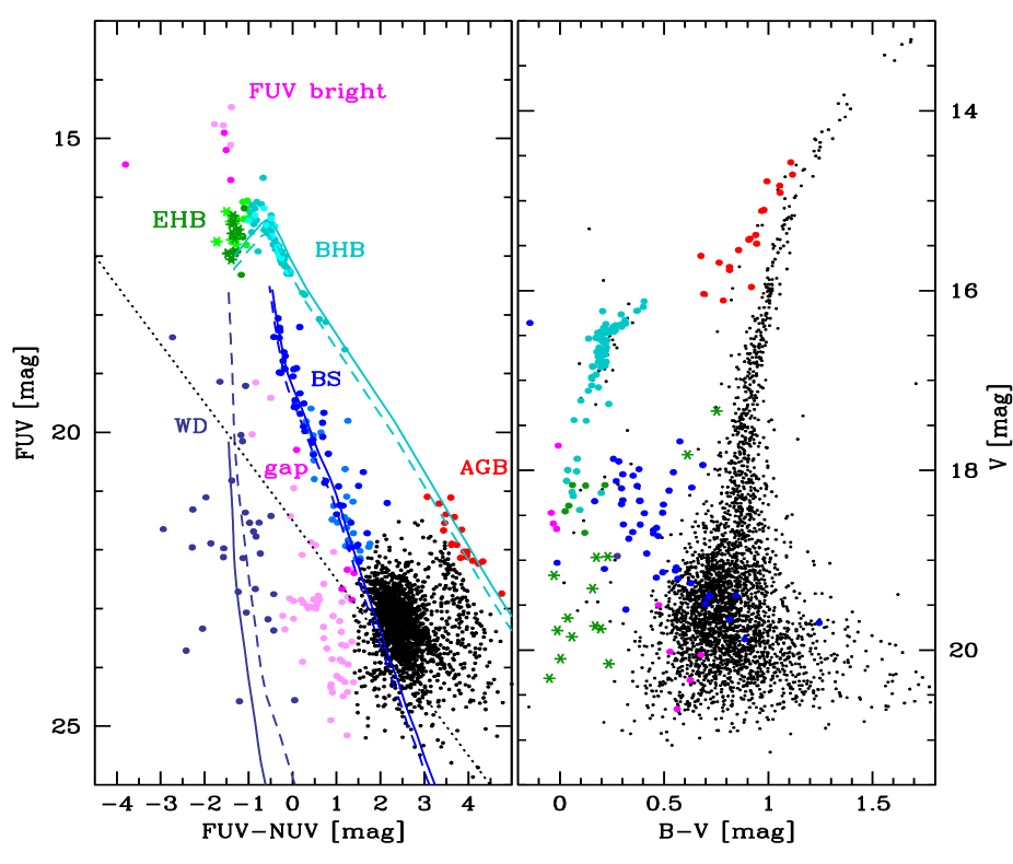
Figure 3: Left panel: $FUV-NUV$ CMD of the core region of M 80. For orientation purposes, we include a theoretical WD and He WD cooling sequence (violet lines), a zero-age main sequence (ZAMS, blue line), and a zero-age HB track (ZAHB, cyan line). BHB stars are plotted in cyan, EHB stars in green, BSs in blue, gap sources (which include CV candidates) in magenta, WD candidates in violet, and AGB stars in red. The $FUV$ bright sources, which are likely AGB manché stars, are plotted in magenta. The remaining sources are MS stars and RGs. $FUV$ sources with optical counterparts are plotted in a darker shade of the same color (except for MS stars and RGs). Right panel: Optical CMD of M 80. The data were taken from Piotto et al. (2002), only the PC data are plotted. The counterparts to the $FUV$ sources are plotted in the same color as in the left diagram. See the text for details.

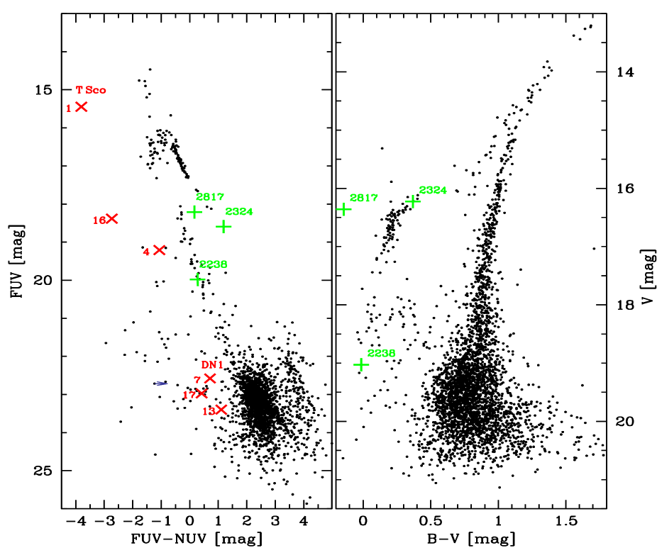
Figure 4: Same as Fig. 3, but with the variable sources marked with green crosses and their $FUV$ id. The most likely counterparts to the X-ray sources are marked with tilted red crosses and their X-ray source id. The WD candidate that is located on the rim of the repeller wire shadow in the $NUV$ image, and that might thus actually be $NUV$ brighter and redder, is marked with a small violet arrow. See the text for details.

The $FUV-NUV$ CMD of the core region of M 80 is shown in Figs. 3 and 4 (left diagrams). For orientation purposes, we include a theoretical zero-age MS (ZAMS, plotted in blue in Fig. 3) and a WD (solid violet line in Fig. 3) and Helium white dwarf (He WD) cooling sequence (dashed violet line). For all our synthetic tracks we adopted a distance of 10 kpc, a reddening of $E_{B-V}=0.18$ mag and a cluster metallicity of $[Fe/H]\simeq-1.7$ (Harris 1996). For details on these tracks, see Dieball et al. (2005a). We also plot a zero-age HB (ZAHB, cyan line) which was constructed based on the $\alpha$ enhanced BaSTI ZAHB model for [Fe/H]=1.62 dex and a mass loss parameter $\eta=0.4$ (e.g. Cordier et al. 2007). We then used synphot within IRAF to calculate the corresponding $FUV$ and $NUV$ STMAGs. As can be seen in Fig. 3, the ZAHB and ZAMS appear to be somewhat brighter and/or redder. Increasing the distance makes the ZAHB and ZAMS fainter, whereas decreasing the reddening makes the tracks brighter and bluer. We found that using a somewhat larger distance of 11.5 kpc and slightly smaller reddening of $E_{B-V}=0.17$ mag for the ZAHB and ZAMS, plotted as dashed tracks in Fig. 3, gives a better fit to our data. However, we point out that the synthetic tracks are plotted for orientation purposes, and - given the difficulties in calibrating the $UV$ data - we do not aim to (re)determine distance and reddening from our $FUV-NUV$ CMD.

The $FUV-NUV$ CMD clearly contains various stellar populations, including WD candidates (violet data points in Fig. 3, left diagram), BSs (blue data points), HB stars (plotted in green and cyan), and AGB stars (red) that are located at the faint and red end of the ZAHB. The CMD also contains a group of objects between the WD cooling sequence and the ZAMS. This is the expected location of WD – MS binaries. We call these objects “gap sources” because the CMD alone does not allow us to distinguish between mass exchanging binaries (CVs) and non-interacting WD binaries (see, e.g. Dieball et al. 2007). The remaining sources (black data points) in the $FUV-NUV$ CMD are MS stars and RGs. The MS turnoff is at $FUV\approx 22.5$ mag and can be recognized by the sudden increase in source numbers along the ZAMS around that magnitude. Our CMD reaches approximately 2.5 mags fainter than the MS turnoff in the $FUV$.

The optical CMD is shown in the right panel of Figs. 3 and 4. The optical counterparts to $FUV$ objects are marked with the same color as in the $FUV-NUV$ CMD. The location of the stellar populations in the optical CMD agrees well with what we expect based on the $FUV-NUV$ CMD, e.g. the counterparts to the $FUV$ BHB stars are on the optical BHB as well, and also the location of the EHB, AGB, and BS stars agrees in both the $FUV-NUV$ and the optical CMD.

In the following subsections, we will discuss the HB, BS, WD and gap source populations in more detail. The selection of stars belonging to the various populations is based on the $FUV-NUV$ CMD, but the numbers we give for the populations should not be taken as exact, since the various zones in the $FUV$ CMD overlap and the discrimination between them can be difficult.

3.1 The Horizontal Branch in the $FUV$

Our $FUV-NUV$ CMD contains a significant population of both EHB and BHB stars located along the bright ($FUV<19$ mag) part of the ZAMS. We define stars to be EHB stars if they have colors at least as blue as the ZAHB at $T_{eff}\approx 20,000$ K (e.g. Momany et al. 2004), corresponding to $FUV-NUV=-1.0$ mag in our CMD. As can be seen in Fig. 3, the optical CMD shows a large gap along the vertical BHB/EHB tail, as was already noted by Ferraro et al. (1998). This gap appears in the $FUV-NUV$ CMD as well and occurs around the “knee” of the ZAMS at $FUV-NUV\approx-0.7$ mag. In both the $FUV-NUV$ and the optical CMD, another, optically fainter and $FUV$ bluer gap is visible. In the $FUV-NUV$ CMD, the bluer gap occurs in the EHB part of the ZAHB sequence approximately at $FUV-NUV\approx-1.2$ mag, corresponding to $T_{eff}\approx 26,000$ K in our model. Sources with (photometrically) hotter $T_{eff}$ are plotted as stars in both CMDs. We refer to these sources as EHB2 stars. EHB stars redder than the optical faint/$FUV$ blue gap are denoted EHB1 stars (see Sect. 5). As can be seen, the bluer EHB2 stars agree very well with the optically fainter EHB stars. Two of the optical counterparts to the EHB2 stars are located in the BS region close to the RGB and might be mismatches.

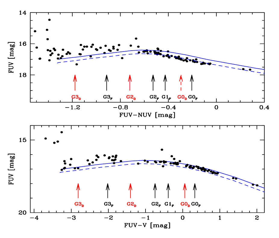
Figure 5: Top panel: $FUV-NUV$ CMD zoomed in on the HB of M 80. Bottom panel: $FUV-V$ CMD of the HB. In both panels, the gaps G_F suggested by Ferraro et al. (1998) are marked with black arrows according to their temperatures. Their location does not agree with the gaps G_D, marked with red arrows, in our CMDs, but instead are slightly shifted. See the text for details.

Fig. 5 (top panel) shows a zoom on the Horizontal Branch in our $FUV-NUV$ CMD. For comparison, we plot the $FUV-V$ CMD in the bottom panel and mark the location of the gaps visible in our data, and of the four gaps described in Ferraro et al. (1998) according to their temperatures along the BaSTI ZAHB. All gaps are marked with a solid arrow in both the $FUV-V$ and $FUV-NUV$ CMDs and are denoted as _D if identified in our data, and _F if referring to the gaps discussed in Ferraro et al. 1998. None of the gaps visible in our CMD appear at the same temperatures as suggested by Ferraro et al. (1998), instead we found that the gaps appear to be somewhat shifted. Ferraro et al. (1998) suggested a temperature of 9500 K for their gap G0_F. We see a gap close to this temperature position only in the $FUV-V$ data at 10000 K, our gap G0_D, but this gap is not visible in our $FUV-NUV$ CMD. G1_F, at 11000 K in Ferraro et al. (1998), cannot be identified in our $FUV-V$ CMD, but we caution that the low number of BHB stars between $-0.5>FUV-V>-1.5$ prevent a secure detection. Our $FUV-NUV$ CMD does not indicate a gap in that area. As already noted, a large gap is visible around $FUV-NUV\approx-0.7$ and $FUV-V\approx-1.4$ that we denote G2_D. According to the temperatures along the ZAHB, this G2_D is in between Ferraro’s G2_F and G3_F gap. Also, in our data G3 appears at somewhat bluer colours and higher temperatures. Table 4 gives an overview of the temperatures assigned to the gaps in Ferraro et al. (1998, their Fig. 4) and this work, all colours refer to the corresponding temperatures based on the BaSTI ZAHBs. Please note that Ferraro et al. (1998) shifted their M 80 $FUV-V$ CMD to match that of M 13, and they also use a different $FUV$ filter (the WFPC2 F160BW). The differences between the exact temperature location of the gaps is likely due to differences in the $FUV$ filter, the HB models used (Ferraro et al. used the Dorman et al. 1993 models, whereas we use the newer BaSTI models), the parameters assumed for the HB model (distance, reddening), and also the calibration of the data. As can be seen, the BaSTI ZAHB fit the $FUV-V$ data somewhat better than the $FUV-NUV$ data, suggesting that the $NUV$ aperture correction might be underestimated, rendering the $FUV-NUV$ color too blue. Keeping this in mind, the temperatures assigned to the gaps (G0 and G2) match relatively well, except for the bluest gap G3 which we found at higher $T_{eff}$, more comparable to the G3 gap in NGC 2808 (see Ferraro et al. 1998, their table 2).

Table 4: Gap colors and temperatures in our $FUV-NUV$ and $FUV-V$ CMDs (cols. 2 – 4). Col. 5 denotes the color corresponding to the temperature associated with the Ferraro et al. (1998) gaps.

	this paper			Ferraro et al. 1998
	FUV-NUV	FUV-V	$T_{eff}$	FUV-V	$T_{eff}$
G0	–	0.059	10000	0.329	9500
G1	–	–	–	-0.389	11000
G2	-0.721	-1.405	14500	-0.743	12000
G3	-1.178	-2.814	25500	-2.019	18000

Based on the WFPC2 data presented by Ferraro et al. (1998), Momany et al. (2004) suggested that M 80 might contain BHk stars. BHk stars are as blue as the EHB stars, but $FUV$ fainter (see Brown et al. 2001). If these stars exist in M 80, our observations show they are very rare. Our $FUV-NUV$ CMD shows only one star that is fainter than the hot end of the ZAHB. This could either be a somewhat fainter but “normal” EHB star, or a BHk candidate. Unfortunately, we did not find an optical counterpart for this source. Definite BHk stars have so far only been found in the most massive GCs, although the number of GCs surveyed does not allow one to conclude that lower mass GCs are incapable of producing BHk stars (see Dieball et al. 2009).

3.2 Blue Stragglers

Fig. 3 shows a well defined trail of stars above the MS turnoff and around the ZAMS, with a few sources located slightly to the red of the ZAMS. This is the expected location of BSs in a CMD if they are produced via the collision or coalescence of two or more lower-mass MS stars. As they are more massive than the MS stars, we expect them to be slightly evolved. We have marked 75 sources as likely BSs; 47 of these have optical counterparts which agree very well with the expected location in the optical CMD. Some of the optical counterparts are fainter than the optical MS turnoff. These are likely BSs with progenitors less massive than the MS turnoff mass. BSs in GCs are thought to be formed dynamical via stellar collisions and/or from evolution of primordial binaries. It is still subject to discussion which is the dominant formation mechanism, if there is one. Recent studies have found no correlation of BSs numbers (or frequencies) with the collision rate, arguing against dynamical formation as the dominating channel (Piotto et al. 2004, Leigh et al. 2007), but on the other hand the radial distribution of BSs seems to be bimodal in many clusters, with a strong central peak, indicating that dynamics play an important role in the formation of BSs in the cores of these clusters (e.g. Dalessandro et al. 2008, Mapelli et al. 2006, Lanzoni et al. 2007, Ferraro et al. 2004).

Ferraro et al. (1999) found an unusual large and centrally concentrated fraction of BSs in M 80 (305 BSs in their WFPC2 dataset). They suggest that these BSs are collisionally formed, and that M 80 is currently in a transient dynamical state where core collapse is delayed via stellar interactions which led to the formation of the large number of BSs (but also see Knigge et al. 2009, who suggest that most BSs - even in the core of GCs - are descended from binary stars, although they do not rule out stellar dynamics as a key factor in the formation and evolution of the parent binaries). More recently, Ferraro et al. (2003) compared six GCs (M 3, M 80, M 10, M 13, M 92, and NGC 288) and found that M 80 has the largest and most concentrated population of BSs. We compare our $FUV$ M 80 data to our $FUV$ M 15 data, which covered a similar field of view as well, and do not find a remarkable excess in BSs. In both M 80 and M 15 we find the same number of BSs (75), but the two clusters are different in the sense that M 15 is even more massive, more concentrated, and more metal-poor compared to M 80. Scaling with the field size at the distance of the cluster, the ratio of BS numbers in M 80 and M 15 is only slightly above unity and not significantly different from the ratio obtained for WDs, for example (see Table 5). This, at first glance, argues against an anomalous enhancement of BS numbers in M 80, at least compared to M 15. On the other hand, if the BS specific frequencies as defined in Ferraro et al. (1999), $F^{BS}_{HB}=N_{BS}/N_{HB}$, are considered, M 15 shows a slightly lower BS specific frequency. This agrees with Piotto et al. (2004) who found an anticorrelation of BS frequency and cluster mass, and a (mild) tendency of increasing BS frequency with decreasing central density. However, allowing for a Poisson error on the number of stars found within the clusters, the difference between the $F^{BS}_{HB}$ is $0.08\pm 0.12$. Thus, although the difference in $F^{BS}_{HB}$ between M 80 and M 15 seems to reflect the trend discussed in Piotto et al. (2004), it is still not statistically significant.

Table 5: Number of HB and gap sources, WD and BS candidates (cols. 2 – 5) detected in M 15 and M 80, and the number of sources per pc² (cols. 6 – 8). Col. 9 gives the BS specific frequency, cols. 10 – 13 give the cluster distance, metallicity, and the logarithmic core and halfmass relaxation time lg(tc), and lg(th) (Harris 1996), col. 14 the cluster total mass (Gnedin et al. 2002), and col. 15 the the central density lg($\rho_{c}$).

name	HB	gap	WD	BS	$\frac{\rm{gap}}{\rm{pc}^{2}}$	$\frac{\rm{WD}}{\rm{pc}^{2}}$	$\frac{\rm{BS}}{\rm{pc}^{2}}$	$F^{BS}_{HB}$	distance	[Fe/H]	lg(tc)	lg(th)	Mtot	lg($\rho_{c}$)
									[kpc]
M 15	133	48	34	75	26	18.5	40.7	0.564	10.3	-2.26	7.02	9.35	1.19	5.38
M 80	117	59	31	75	34	17.3	43.2	0.641	10.0	-1.77	7.73	8.86	0.50	4.76

3.3 White Dwarfs

We find $\approx 30$ sources that are located close to the WD and He WD sequences in Fig. 3. Most of these are likely to be WDs, although a few could be CVs or detached WD – MS binaries (as we will argue in Sect. 4). The number of expected WDs in our field of view can be estimated from the number of HB stars and the relative lifetimes of stars on the HB and the cooling timescale for WDs. In total, we have 117 HB sources (30 EHB stars, 80 BHB stars and 7 $FUV$ bright sources that are likely AGB manché stars). In making this comparison, we can only consider WD candidates above the completeness limits in both $FUV$ and $NUV$ images. If we therefore restrict our WD sample to a limiting magnitude of $FUV\approx 22$ mag (corresponding to $T_{eff}\approx 24,000$ K and a cooling age of $2\times 10^{7}$ yrs), we find 24 WD candidates in our CMD; which compares very well to the 23 WDs that are expected on the basis of the HB numbers. This suggests that most, if not all, of our candidates are indeed WDs. Note that one of our WDs has an unexpectedly bright optical counterpart with $V\approx 19$ mag. However, the $NUV$ counterpart is located at the rim of the repeller wire shadow in the $NUV$ image, and might thus actually be brighter. In this case, this source would be redder, which would shift it into the BS region in our $FUV-NUV$ CMD. This source is marked with an arrow in Fig. 4 (left diagram).

3.4 Gap Sources - CVs and other WD Binaries

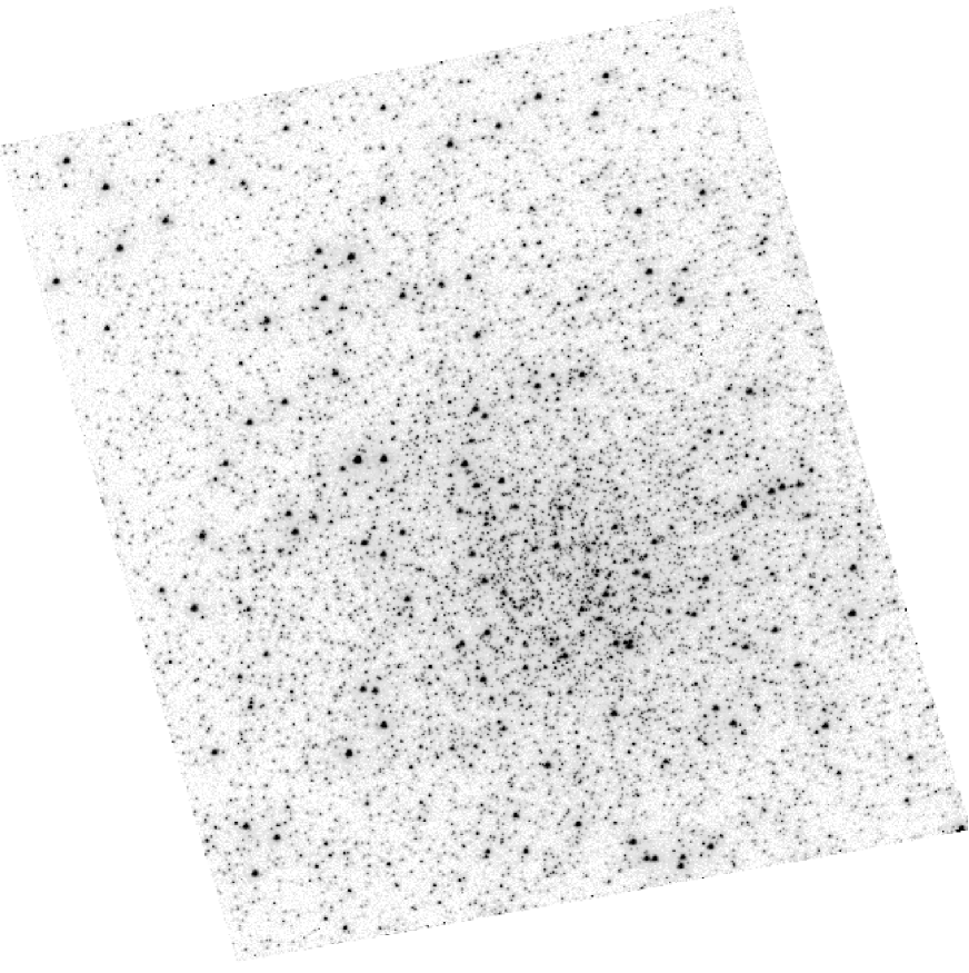
Figure 2: Same as Fig. 1, but for the $NUV$ HRC/F250W. Note that the HRC field of view is somewhat smaller than the SBC field of view with $29\arcsec\times 25\arcsec$.

A number of sources can be seen in the “gap” between the WD cooling sequences and the ZAMS in Fig. 3. As mentioned earlier, we cannot distinguish between the CV candidates and the detached WD – MS binaries, so we call these objects the “gap sources”. How many CV candidates can we expect amongst the $\approx 60$ gap sources? Detailed theoretical work was done on 47 Tuc (di Stefano & Rappaport 1994, Shara & Hurley 2006, Ivanova et al. 2006), investigating various dynamical and primordial formation channels for CVs and predicting a few 100 CVs in this cluster. For the sake of simplicity, we adopt di Stefano & Rappaport’s (1994) prediction of 190 active CVs in 47 Tuc, and scale this number with the capture rate (e.g. Heinke et al. 2003) to M 80. This yields $\approx 100$ CVs that can be expected in M 80. According to di Stefano & Rappaport (1994), approximately half of the captures should take place inside the cluster core. Given that our detection limit corresponds to a white dwarf temperature of $T_{eff}\approx 24,000$ K (see Sect. 3.3), we will only be able to detect relatively bright, long-period CVs above the period gap (Townsley & Bildsten, 2003, their Figs. 1 and 2). About twenty of these long-period CVs should exist in 47 Tuc (Di Stefano & Rappaport, 1994, their Fig. 3 and Table 5). Ivanova et al. (2006) suggested that 35 - 40 CVs should be detectable in the core of 47 Tuc. Scaling these numbers to M 80, we can expect approximately 10 to 20 such sources in the core of M 80. Note that the $NUV$ field of view covers $\approx 1.5$ times the core radius of M 80. Thus, the number of objects we find in the gap region is consistent with the number of predicted CVs. Five of our gap sources have optical counterparts, all of which lie bluewards of the MS and below the optical MS turnoff. These systems might have relatively massive MS companions that dominate the optical light. On the other hand, all five of these sources are located close to the ZAMS in the $FUV$ CMD, making them BS candidates as well.

3.5 Variable Sources

As noted earlier, only few variable sources are known in M 80 (Wehlau et al. 1990, Clement & Walker 1991, Clement et al. 2001), and indeed the region where RR Lyrae stars are expected is unpopulated in our $FUV-NUV$ CMD. Our $FUV$ observations cover four consecutive HST orbits, comprising 32 single images, and we have used these data to search for variable sources. We found three sources that exhibit convincing evidence of variability, namely source no. 2238, 2324, and 2817. These sources are flagged as variable in Table 1, and are marked in Fig. 4. Source no. 2238 shows short-term variability ($\approx 55$ min) and is likely a SX Phoenicis star. Source no. 2324 shows long-term variability and might be a RR Lyrae or a Cepheid. Source no. 2817 is a peculiar object that shows very strong variability. A more detailed study on the variable sources in M 80, including their lightcurves, will be presented in a forthcoming paper (Thomson et al., in preparation).

4 Identification of X-ray Sources

As noted earlier, M 80 was observed with $Chandra$ by Heinke et al. (2003) who identified 19 discrete sources within the half-mass radius of the cluster. All but four of these – CX05, CX08, CX10, and CX19 – are in the field of the $FUV$ image. Since the majority of the X-ray sources are expected to be CVs, and all are thought to be binaries, identifying their counterparts at longer wavelengths is important, and our $UV$ images and source catalogs provide us with an excellent opportunity to accomplish this task.

Heinke et al. (2003) referenced the X-ray source positions in M 80 to a bright star (HD146457) in the Tycho catalog that was roughly $4\arcmin$ from the core of M 80, and allowed for an absolute position error of $2\arcsec$. This error is quite large, given the crowding of the core of M 80, so we have attempted to find a more accurate way to register the X-ray sources to our fields. HD146457 is not in the ACS image we used to establish an accurate (Tycho-based) WCS for our UV images of the core of M 80. We therefore compared the positions of the 52 X-ray sources identified by Heinke et al. (2003) outside of the core, which presumably are mostly foreground stars and background quasars, to the ACS WFC 435W field. Eight of these sources are located within the region covered by the WFC image, and two of those, J161658.3-225838 and 161659.8-225931, were near relatively bright stars. The offset between the Heinke positions and these two stars was approximately $0\farcs 13$ in $\alpha$ and $1\farcs 17$ in $\delta$, well within Heinke’s estimated error.

After correcting the Heinke et al. (2003) X-ray source positions by these values, we compared the X-ray sources with the $FUV$ image of M 80. It was immediately apparent that a number of the X-ray sources had counterparts with the brighter sources in the field. Of the fifteen X-ray sources within our $FUV$ field of view, six lie within $1\arcsec$ of a bright $FUV$ source ($FUV<22$ mag) that has no optical counterpart. We then applied a final shift of $0\farcs 1$ to optimally align the three X-ray sources with the most definite $FUV$ counterparts (CX01, CX03 and CX04). (Note that these are 3 of the 4 brightest X-ray sources, and that CX02, the one not associated with a bright $FUV$ source, has a spectrum which suggests it is a quiescent LMXB). The positions of the X-ray sources on the $FUV$ image after these corrections are shown in Fig. 1, where the circles represent the 3$\sigma$ statistical uncertainty in X-ray position as determined by Heinke et al. (2003). As explained in more detail below, there are 6 X-ray sources with bright $FUV$ counterparts, whose identifications we consider secure. The final RMS offset between the X-ray and $FUV$ positions of these 6 sources is only $0\farcs 14$ after alignment.

We then compared the positions of all X-ray sources to those of objects in our $FUV$ catalog, using the 3$\sigma$ statistical uncertainty in X-ray position for each source. Table 6 summarizes the results of this comparison. For some sources, especially those which are faint in X-rays, and hence have larger error circles, multiple sources lie within the 3$\sigma$ radius. In these cases, we have listed all of the possible $FUV$ counterparts in order of increasing distance from the nominal X-ray position. The four Chandra sources which were outside the $FUV$ field of view appear in the table, but only to indicate their improved positions.

Table 6: Chandra X-ray Source Comparison. The X-ray source id is given in the first column, followed by our revised positions for the X-ray sources in cols. 2 and 3, the 3$\sigma$ statistical uncertainty in col. 4, the angular distance from the nominal position to the $FUV$ object in col. 5, the following cols. 6 to 14 are as in Table 1.

1	2	3	4	5	6	7	8	9	10	11	12	13	14
IDX	RA	DEC	$3\sigma$	Offset	IDFUV	$FUV$	$\Delta FUV$	$NUV$	$\Delta NUV$	IDPiotto	B	V	Comments
	[hh:mm:ss]	[deg:mm:ss]	[$\arcsec$]	[$\arcsec$]		[mag]	[mag]	[mag]	[mag]		[mag]	[mag]
CX01	16:17:02.817	-22:58:33.92	0.22	0.02	2129	15.444	0.005	19.247	0.008	*	*	*	FUVbright
CX02	16:17:02.580	-22:58:37.73	0.13	0.08	1523	23.736	0.229	21.247	0.029	*	*	*	MS/RG
CX03	16:17:01.600	-22:58:29.20	0.18	0.05	2818	17.614	0.011	*	*	*	*	*	outside HRC
CX04	16:17:02.008	-22:58:34.28	0.23	0.04	2082	19.209	0.022	20.277	0.024	*	*	*	WD
				0.22	4790	22.589	0.134	18.748	0.007	2190	16.289	15.198	RG
CX05	16:17:01.711	-22:58:16.59	*	*	*	*	*	*	*	*	*	*	*
CX06	16:17:03.573	-22:58:26.55	0.29	0.21	3221	23.656	0.181	21.152	0.031	*	*	*	MS/RG clump
			0.29	0.25	3181	23.448	0.162	21.210	0.024	*	*	*	MS/RG clump
CX07	16:17:02.169	-22:58:38.52	0.27	0.12	1387	22.578	0.120	21.869	0.055	*	*	*	gap
				0.25	4850	22.926	0.159	20.666	0.020	*	*	*	MS/RG clump
CX08	16:17:01.118	-22:58:30.58	*	*	*	*	*	*	*	*	*	*	*
CX09	16:17:02.404	-22:58:33.85	0.44	0.40	2106	18.393	0.015	18.693	0.009	1823	18.510	18.343	BS
CX10	16:17:00.412	-22:58:30.12	*	*	*	*	*	*	*	*	*	*	*
CX11	16:17:02.476	-22:58:39.11	0.43	0.28	1352	22.751	0.137	20.424	0.017	1134	19.980	19.278	MS
				0.33	1341	22.424	0.112	20.209	0.015	1153	19.821	19.296	MS
				0.36	1283	23.065	0.158	20.560	0.033	*	*	*	MS/RG clump
CX12	16:17:02.570	-22:58:46.25	0.43	0.10	214	17.965	0.014	*	*	*	*	*	outside HRC
				0.24	232	16.306	0.006	*	*	*	*	*	outside HRC
				0.33	251	21.981	0.112	*	*	*	*	*	outside HRC
CX13	16:17:01.759	-22:58:30.54	0.42	0.11	2624	23.397	0.182	22.291	0.240	*	*	*	gap
				0.25	2605	24.091	0.264	22.384	0.078	*	*	*	MS/RG clump
CX14	16:17:02.558	-22:58:31.75	0.70	0.30	2414	22.920	0.195	20.882	0.022	1871	20.555	19.802	MS
				0.30	2453	22.237	0.108	19.372	0.009	1946	18.991	18.185	RG
				0.32	2452	17.661	0.011	17.380	0.004	1880	16.596	16.222	BHB
				0.38	2415	22.557	0.125	20.614	0.022	*	*	*	MS/RG clump
				0.42	2512	22.452	0.130	20.186	0.018	1978	20.135	19.291	MS
				0.64	2428	22.337	0.144	20.313	0.015	1935	19.602	18.618	MS
				0.67	2541	23.253	0.346	20.673	0.038	*	*	*	MS/RG clump
CX15	16:17:02.104	-22:58:33.05	0.43	0.15	2269	23.664	0.232	*	*	*	*	*	no NUV
				0.17	2270	22.868	0.146	20.393	0.017	*	*	*	MS/RG clump
				0.17	2294	23.197	0.157	*	*	*	*	*	no NUV
CX16	16:17:02.124	-22:58:21.05	0.70	0.05	3967	16.388	0.007	17.210	0.003	3338	18.350	18.285	BHB
				0.23	4786	18.383	0.020	21.117	0.048	*	*	*	WD
CX17	16:17:02.224	-22:58:34.95	0.68	0.21	1944	22.971	0.235	22.555	0.158	*	*	*	gap
				0.33	2005	22.324	0.157	20.989	0.057	*	*	*	gap
				0.45	1952	23.262	0.221	21.275	0.045	*	*	*	MS/RG clump
				0.47	1911	23.045	0.224	20.214	0.021	*	*	*	MS/RG clump
				0.47	2022	21.579	0.093	18.727	0.007	1975	15.046	13.441	RG
				0.51	1849	16.799	0.008	18.082	0.004	*	*	*	EHB
				0.52	2050	22.752	0.209	20.713	0.026	*	*	*	MS/RG clump
				0.53	4791	22.211	0.116	20.005	0.022	*	*	*	MS/RG clump
				0.61	1918	22.741	0.155	20.124	0.014	*	*	*	MS/RG clump
CX18	16:17:02.824	-22:58:37.25	0.68	0.35	1559	23.374	0.221	20.390	0.027	*	*	*	MS/RG clump
				0.38	1659	23.318	0.178	20.465	0.016	1013	20.127	19.329	MS
				0.45	1601	22.161	0.090	18.628	0.005	999	16.279	15.166	RG
				0.46	1531	22.672	0.122	20.249	0.020	923	19.973	19.245	MS
				0.64	1607	20.351	0.040	19.881	0.012	*	*	*	BS
CX19	16:17:03.854	-22:58:48.35	*	*	*	*	*	*	*	*	*	*	*

4.1 CX01: The Nova T Sco

CX01 is particularly interesting since it is located near the site of nova T Sco, which is one of only two novae known to have occurred along the line of sight to a galactic globular cluster. Based on an analysis of the historical and HST WFPC2 data, Shara & Drissen (1995) obtained two estimates of the position of the nova, one based on the offset of the nova from the cluster center, the other based on offsets from two nearby stars. Based on their estimates of the nova position, they identified a blue star as the likely post-nova system. Using the finding chart provided in Shara & Drissen (1995), we identified this blue star as source no. 2422 in our $UV$ catalog.

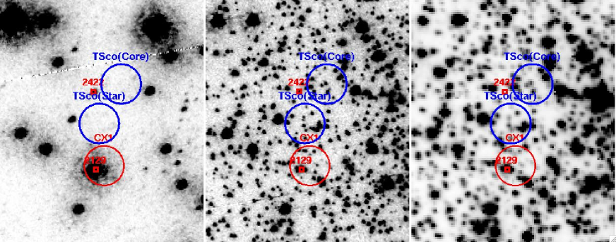
Figure 6: The portion of the $FUV$ (left), $NUV$ (middle) and ACS WFC 435W (right) image where the nova T Sco was seen. Shara & Drissen (1995) suggested that a very blue star, easily visible in our $FUV$ and $NUV$ images as object 2422, was likely to be the CV responsible for the nova. They also used the historical data to make two estimates of the location of the nova within the cluster, one based on the location of the cluster core and another based on offsets from nearby stars. These are labelled in blue. Our astrometry suggests that another very blue object, source no. 2129, is more likely to be the brightest X-ray source in the globular cluster, marked with a red circle. Given the uncertainties in locating the nova from the historical record, our object 2129 seems a better candidate as the CV which gave rise to the nova.

The region containing CX01 and the site of the nova is shown in Fig. 6. In order to locate the likely position of the nova in our frames, we offset the Shara & Drissen (1995) locations for the nova to our Tycho-based coordinate system using the difference in the position of the two astrometric reference stars discussed by Shara & Drissen (1995). In our coordinate system, the historical nova position as estimated from the offset to the cluster core is $16^{h}17{m}02.80^{s}$ $-22^{\circ}58\arcmin 32.21\arcsec$ (J2000) and the position estimated from the two nearby stars is $16^{h}17^{m}02.84^{s}$ $-22^{\circ}58\arcmin 33.21\arcsec$.

Shara & Drissen’s (1995) object is located close to both positions and is indeed very blue. More specifically, it has $FUV=19.14\pm 0.02$ mag and $FUV-NUV=-1.65$ mag, which places it slightly on the blue side of the WD sequence in Fig. 3; we have classified it as a hot WD, a region of the CMD that could indeed contain CVs. However, given the proximity of the brightest X-ray source, CX01, to the nova position, it seems highly likely that CX01 is, in fact, associated with the old nova CV system that produced the 1860 eruption. As shown in Fig. 6, the position of Shara & Drissen’s (1995) object is inconsistent with that of CX01. Moreover, Shara & Drissen (1995) had already noted that, at M${}_{B}=+6.8$, their source was about 10 times fainter than canonical old novae.

On the other hand, CX01 has a position that is consistent with source no. 2129, which is one of the ten brightest objects in our $FUV$ catalog, at $FUV=15.44\pm 0.01$ mag. Furthermore, as shown in Fig. 4, this is the bluest source in our CMD ($FUV-NUV=-3.80$ mag). This is actually unphysically blue (i.e. significantly bluer than an infinite temperature blackbody, which has $FUV-NUV=-1.8$ mag), suggesting that the object must have been much brighter during the $FUV$ observations than during the $NUV$ observations a month later. This is surely the counterpart to CX01, and its variability is consistent with the suggestion by Heinke et al. (2003) that this particular source is a CV. The source is close to Shara & Drissen’s (1995) preferred position for the nova, based on offsets from nearby stars, and, since this is the type of object that would be expected to produce a nova, is a much more viable candidate for the quiescent nova than the blue object identified by Shara & Drissen (1995). It is also about 1.5 mag brighter in the $NUV$ than the candidate described by Shara & Drissen (1995) and therefore closer to the quiescent magnitude of other novae. Given its position, X-ray and UV brightness and variability, this source is almost certainly the true counterpart to T Sco. It clearly merits further study.

4.2 CX04, CX07, CX13, CX16, CX17: Cataclysmic Variables

All of the 15 Chandra sources in the $FUV$ field of view have at least one possible $FUV$ counterpart amongst the $\simeq 3000$ objects in our $FUV$ catalog if we adopt the 3$\sigma$ X-ray error circle as a criterion for identifying candidate matches. Thus, it is obvious that one cannot assume that the identifications suggested in Table 6 are real, without considering the magnitude of the difference in position or the nature of the object. However, CVs are expected to be found only amongst the gap sources (59 objects) and the WD candidates (31 objects) in our $FUV$-$NUV$ CMD. Given that three X-ray sources (CX07, CX13, CX17) are associated with gap sources and a further two (CX04, CX16) with WD candidates, we regard these identifications as secure.

The $FUV$ counterpart to CX07 is one of the sources identified with a gap object (no. 1387 in our catalog, with $FUV=22.58$ mag). This $FUV$ object lies only $0\farcs 12$ from the best X-ray position. There is no reason to suspect that the other possible candidate, source no. 4850, which lies in the RG/MS clump, would have been detected as an X-ray source. As it happens, however, there is more information in this case. Source no. 1387 was previously identified by Shara et al. (2005) as a CV, which they observed to have undergone a DN outburst. (The other DN they identified in M 80 is not within our $FUV$ field of view.) They suggested that this object, which they called DN1, was associated with CX17, which is nearby. Our more accurate X-ray positions make it clear that CX07, and not CX17, is the X-ray source associated with the dwarf nova.

4.3 Other X-ray Sources with $FUV$ Counterparts

There are seven Chandra sources – CX02, CX06, CX09, CX11, CX14, CX15, and CX18 – that are inside both the $FUV$ and $NUV$ fields of view but have no obvious counterparts. In each case, there is at least one object within the 3 $\sigma$ error circle but the counterparts are neither very bright nor in a region of the CMD expected to be populated by CVs or UV-bright X-ray sources. In several of the cases, there are no candidates within the 1 $\sigma$ error circle, and this makes their association with the sources listed in Table 6 less likely.

Of these sources, CX02 and CX06 are arguably the most interesting. Both were identified by Heinke et al. (2003) on the basis of their hard X-ray spectra and luminosities as possible quiescent LMXBs. Such objects also are expected to have high values of $F_{X}/F_{opt}$. The only possible counterparts to these objects are classified by us as in the MS/RG group, and none of these is within the 1 $\sigma$ error circle of the X-ray sources. This result is consistent with the suggestion that they are indeed quiescent LMXBs.

Two further X-ray sources, CX03 and CX12, are located in regions where there is no $NUV$ coverage. There is a bright $FUV$ object associated with each of them, but we we cannot classify the object in our $FUV-NUV$ CMD.

5 Radial Distributions and Masses of the Stellar Populations

5.1 Radial Distributions

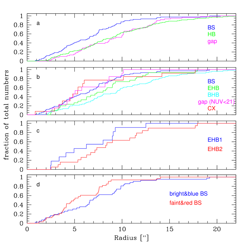
Figure 7: Cumulative radial distributions of the various stellar populations that show up in our $FUV-NUV$ CMD, and of the X-ray sources. We only compare the BS candidates, gap objects, HB stars and X-ray sources. Panel (a) shows the radial distribution of BSs, HB stars and gap sources. Panel (b) shows the BHB and EHB populations, the magnitude selected ($NUV<21$ mag) gap sources, the BSs and X-ray sources. Panel (c) compares the EHB1 and EHB2 populations. Panel (d) compares the radial distribution of the bright/blue BSs and the faint/red BSs. Contrary to our expectation, we see the faint (red) BSs to be stronger concentrated than the bright (blue) BSs. See the text for the details.

The radial distribution of the various stellar populations that show up in our CMD, and also of the X-ray sources, are plotted in Fig. 7. As our CMD is limited by the $NUV$ data, we also present the radial distributions for sources brighter than 21.5 mag in the $NUV$. This selection affects only the gap sources. We compare the BS candidates, the gap sources, and EHB and BHB stars. WD and MS populations are not shown as both distributions suffer from incompleteness in the $FUV$ especially in the core region of M 80 due to the concentration of bright stars. Such faint sources are not detectable close to the bright stars because of the broad wings of the $FUV$ PSF, see Sect. 2.

In order to assess the statistical significance of the differences between the various stellar populations, we applied Kolmogorov-Smirnov (KS) tests. The KS test measures the probability that two sample populations are drawn from the same underlying distribution. Thus the larger the probability, the more similar the two populations, whereas small probabilities signal significantly different distributions. The number of sources in the various distributions in the full and magnitude selected samples are given in Table 7; the results from the KS tests are presented in Table 8.

Table 7: Number of sources in the various populations, both in the full samples and the magnitude selected sample with $NUV<21.5$ mag.

	all	$NUV<21.5$
BS	75	75
BHB	80	80
EHB	30	30
EHB1	11	11
EHB2	19	19
gap	59	13

Table 8: KS probability in % that populations have similar radial distributions.

	all	$NUV<21.5$
BS–gap	0.06	95.1
BS–HB	0.2	0.2
BS–BHB	0.02	0.02
BS–EHB	28.5	28.5
BS–CX	21.7	21.7
gap–HB	79.9	7.0
gap–BHB	77.5	4.0
gap–EHB	23.4	40.2
gap–CX	0.9	82.8
HB–CX	0.3	0.3
BHB–EHB	9.1	9.1
BHB–CX	0.2	0.2
EHB–CX	4.4	4.4
EHB1–EHB2	49.5	49.5
bBS–fBS	3.5	3.5

Fig. 7 shows all of the radial distributions. The BS stars are clearly the most centrally concentrated population. A strong concentration of the BSs was already noticed in Ferraro et al. (1999).

In the magnitude-limited sample (Fig. 7, panel b), X-ray and gap sources (which include the CV candidates) and BSs are the most concentrated populations. In fact, the KS test does not suggest a strong difference between these three populations (see Table 8). A strong central concentration of BSs and CVs is to be expected for two reasons. First, a significant fraction of these objects may be formed in stellar dynamical interactions that preferentially take place in the dense cluster core. Second, BSs (merged MS stars) and bright CVs (composed of a WD and near-MS star) are more massive than ordinary cluster members and will thus sink to the core due to mass segregation.

No significant differences are found between the radial distributions of the various HB populations.

5.2 The Peculiar Blue Straggler Population: Bright versus Faint Blue Stragglers

Bright BSs are thought to be more massive than faint BSs (e.g. Sills et al. 2000). They are also thought to be younger than the faint BSs, see e.g. Ferraro et al. (2003, their Fig. 4). Provided that the ages of all the BSs are larger than the cluster relaxation time $t_{halfmass}$, the bright, massive BSs should thus be more centrally concentrated than the fainter, less massive BSs due to mass segregation. We decided to test this hypothesis.

Since bright BSs are also bluer (and hotter) than faint BSs, we created our bright BS sample by selecting BSs with $FUV-NUV<0.9$ mag, and a corresponding faint BS sample by selecting BSs with $FUV-NUV>0.9$ mag. Nearly all of the $FUV$ bright and blue BSs are also optically brighter than $V=19$ mag (28 out of 33 of the bright and blue BSs with optical counterparts), and most of the $FUV$ faint and red BSs are also optically fainter than $V=19$ mag (11 out of 14 with optical counterparts).

Fig. 7, panel d, shows the radial distribution of the bright and faint BSs. Surprisingly, the faint BSs (red line) are more concentrated than the bright BS (blue line). The KS-test suggests that there is only a 3.5% probablility that both the faint and the bright BSs are drawn from the same parent distribution, see Table 8. In order to test the sensitivity of this result to the adopted cluster center, we carried out a Monte Carlo simulation. In each iteration, we shifted the cluster center randomly in line with the error derived in Sect. 2.4, computed the corresponding new distance from the cluster center for each BS and then calculated the corresponding KS probability for the faint/red and bright/blue BS radial distribution. The outcome of 100,000 of these iterations was that 63% of the iterations yielded KS probabilities below 4.6%, i.e. better than a $2\sigma$ level of confidence. Thus, the marginally significant difference we find between the radial distributions of these two types of BSs is not very sensitive to the exact choice of the cluster center.

This result is rather puzzling. A tentative explanation could be that BSs get a kick at their formation. This could work, since the bright BSs are younger and have shorter lifespans than the faint BSs. Thus, if their initial kick takes BSs out to regions where the relaxation timescale is shorter than the typical age of faint BSs, but longer than that of bright BSs, the latter will not have had time to sink (back) to the core. In any event, we urge others to search for a similar effect in other globular clusters.

5.3 Mass Estimates

The typical mass of objects belonging to a particular stellar population can be estimated by analyzing their radial distribution. Assuming that the distributions for all masses can be approximated by King (1966) models, we can then compare the distributions of different populations to infer the ratio of their typical masses. Here, we follow Heinke et al. (2003) and compare our source distributions to “generalized theoretical King models”:

$S(r)=\int{(1+(\frac{r}{r_{c\star}})^{2})^{\frac{1-3q}{2}}}dr$

where $q=M_{X}/M_{\star}$, $M_{\star}$ is the mass of the stellar population that defines the core radius $r_{c\star}$, and $M_{X}$ is the mass of the source population for which we want to find the mass.

We adopt a core radius of $r_{c\star}=6\farcs 5$ as determined by Ferraro et al. (1999) from fitting a King model (1996) to their WFPC2 data, and we assume that the core radius is defined by MS turnoff stars with $M_{\star}=0.8M_{\odot}$. In order to have as much radial coverage as possible, we have corrected the distribution to account for the fractional area covered by the actual field of view of the instrument as a function of radius.

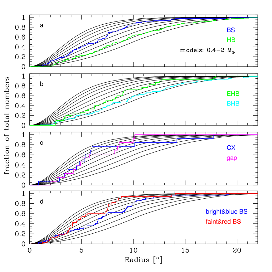
Figure 8: Comparison of the source distribution with theoretical King models for stellar populations with average masses ranging from $0.4M_{\odot}$ (bottom black line in each panel) to $2M_{\odot}$ (top black line), in steps of $0.2M_{\odot}$. BS and HB populations are plotted in panel (a). As can be seen, the BS population agrees well with a model of mass $1.2M_{\odot}$, and the HB stars with masses around $0.6M_{\odot}$. Panel (b) shows the EHB and BHB population. EHB stars seem to be slightly more massive ($0.8M_{\odot}$) than BHB stars ($0.6M_{\odot}$). Panel (c) shows the X-ray and the magnitude selected gap sources. Both source populations seem to be more massive than $1M_{\odot}$. Panel (d) shows the bright vs. faint BSs. Surprisingly, the faint BSs seem to be more massive ($\approx 1.4M_{\odot}$) than the bright BSs ($\approx 1M_{\odot}$). See the text for details.

The area corrected models are plotted in Fig. 8, with the radial distributions of the BS, HB, gap and X-ray source populations overplotted. To avoid confusion, we compare only two source populations per panel in Fig. 8. BS and HB distributions are plotted in panel a. The BS population agrees well with a model of mass $1.2M_{\odot}$, while the distribution of HB stars implies masses around $0.6M_{\odot}$. Both of these numbers are reasonable and agree with an average mass estimate based on the mass distribution along the ZAMS and the ZAHB.

In panel b, we show the EHB and BHB population. EHB stars seem to be more massive with $\approx 0.8M_{\odot}$ than BHB stars ($0.6M_{\odot}$) (but recall that the difference between these distributions is not statistically significant). This is contrary to the mass distribution along the ZAHB, which suggests that the BHB stars span a mass range of $\approx 0.63\rm{M}_{\odot}$ to $\approx 0.52\rm{M}_{\odot}$, resulting in an average mass of $\approx 0.58\rm{M}_{\odot}$. Stars become less massive towards the end of the ZAHB, so that the EHB stars, on average, should have a mass less than $\approx 0.51\rm{M}_{\odot}$.

The radial distribution of X-ray sources and of the magnitude-limited sample of gap sources are plotted in panel c. Both source populations seem to be more massive than $1M_{\odot}$, but a more accurate estimate is not possible based on our Fig. 8. Our result broadly agrees with Heinke et al. (2003) who suggested an average mass of $1.2\pm 0.2M_{\odot}$ for the X-ray source population.

The $FUV$ bright vs. $FUV$ faint BSs are compared in panel d. Based on this plot, it seems that the faint BSs are more massive ($\approx 1.4M_{\odot}$) than the bright & blue BSs ($\approx 1M_{\odot}$). A mass estimate based on the mass distribution along the ZAMS suggests that the faint and red BSs cover a mass range of 0.94 to 1.13 $\rm{M}_{\odot}$, resulting in an average mass of $\approx 1.04\rm{M}_{\odot}$, whereas the bright and blue BSs should be more massive, spanning 1.13 to 1.55 $M_{\odot}$ with an average of $\approx 1.34\rm{M}_{\odot}$. Again, this is contrary to the mass estimate based on the radial distribution. However, all of the estimates based on the radial distributions only hold if the populations have reached thermal equilibrium. In the “kick” scenario sketched in the previous section (to account for the unexpected difference between bright and faint BS distributions), the bright BSs do not satisfy this condition.

6 Conclusions

We analyzed deep $FUV$ and $NUV$ images of the core region of M 80. We have astrometrically corrected our master images to the Tycho based WCS, and identified 3168 sources in the $FUV$ master image, of which 2345 have counterparts in the somewhat smaller $NUV$ master image of M 80. We have also found optical counterparts for 1268 of the sources in our $FUV-NUV$ CMD.

The $FUV-NUV$ CMD shows a rich variety of stellar populations in M 80. Among the objects are 75 BS candidates, 80 BHB and 30 EHB stars, 31 WD candidates, and 59 objects in the gap between the WD and MS. The numbers of bright WDs (24) and of gap sources are consistent with theoretical predictions. The $FUV-NUV$ CMD reveals clear gaps along the BHB and EHB (at $T_{eff}\approx 14,500$ K and $\approx 25,500$ K) which can also be identified in the optical CMD. M 80 does not appear to have a population of blue hook stars in its core, as only one possible BHk candidate was found.

Overall, the BS stars are the most centrally concentrated population, with their radial distribution suggesting a typical blue straggler mass of about $1.2~{}M_{\odot}$. Ferraro et al. (1999, 2003) suggested that M 80 comprises an unusual large and concentrated population of BS stars, compared to other clusters, and suggest that M 80 is currently in a transient dynamical state where core collapse is delayed via stellar interactions that formed the large number of BSs. We compared our $FUV$ M 80 data to our $FUV$ M 15 data, which covered a similar field of view, and do not find a remarkable excess in BSs. However, counterintuitively, we found that the faint and red BSs are significantly more centrally concentrated than the bright and blue BSs, with only a 3.5% probablility that faint and bright BSs are drawn from the same distribution. This result is surprising. One possible explanation could be that the bright BSs get a kick at their formation which takes them out to regions where the relaxation timescale is longer than the typical age of bright BSs but shorter than the typical age of faint BSs. In that case, the bright BSs would not have had time to settle towards the cluster core.

Finally, we believe we have recovered the object that was responsible for the Nova 1860 AD, also known as T Scorpii. It is not the UV bright object identified by Shara & Drissen (1995), but rather a dwarf nova located at the site of the historical event, which is today the brightest X-ray object, CX01, in M 80, see Heinke et al. (2003). This object, source no. 2129, is one of the brightest and the bluest $FUV$ source in our catalog. This identification has also enabled us to clearly identify the $FUV$ objects associated with another 5 of the 15 X-ray sources located in the core of M80. We found that CX04, CX07, CX13, CX16 and CX17 are associated with gap sources and WDs. All of these are likely CVs. Our source no. 1387 coincides with the dwarf nova DN1 observed by Shara et al. (2005) and is the counterpart to CX07. For seven X-ray sources (CX02, CX06, CX09, CX11, CX14, CX15, and CX18) the $FUV$ counterparts are not obvious. The two remaining X-ray sources, CX03 and CX12 are located in regions where there is no $NUV$ coverage. There is a bright $FUV$ object associated with each of them, but we can not classify the object in our $FUV-NUV$ CMD. The radial distributions of the 15 X-ray sources and of the brighter gap sources ($NUV>21.5$ mag) are not statistically different and suggest masses $>1M_{\odot}$.

References

- Alcaino et al. (1998) Alcaino, G., Liller, W., Alvarado, F., Kravtsov, V., Ipatov, A., Samus, N. & Sminrov, O. 1998, AJ, 116, 2415
- Brocato et al. (1998) Brocato, E., Castellani, V., Scotti, G. A., Saviane, I., Piotto, G. & Ferraro, F. R. 1998, A&A, 335, 929
- Brown et al. (2001) Brown, T. M., Sweigart, A. V., Wayne B. L. & Hubeny, I. 2001, ApJ, 562, 368
- Cavallo et al. (2004) Cavallo, R. M., Suntzeff, N. B. & Pilachowski, C. A. 2004, AJ, 127, 3411
- Clement & Walker (1991) Clement, C. M. & Walker, I. R. 1991, AJ, 101, 1352
- Clement et al. (2001) Clement, C., Muzzin, A., Dufton, Q. et al. 2001, AJ, 122, 2587
- Cordier et al. (2007) Cordier D., Pietrinferni A., Cassisi S. & Salaris M. 2007, AJ, 133, 468
- Dalessandro et al. (2008) Dalessandro, E., Lanzoni, B., Ferraro, F. R., Rood, R. T., Milone, A., Piotto, G. & Valenti, E., 2008, ApJ, 677, 1069
- Dieball et al. (2005a) Dieball, A., Knigge, C., Zurek, D., Shara, M.M. & Long, K. 2005a, ApJ, 625, 156
- Dieball et al. (2005b) Dieball, A., Knigge, C., Zurek, D., Shara, M.M. & Long, K. 2005b, ApJL, 634, L105
- Dieball et al. (2007) Dieball, A., Knigge, C., Zurek, D., Shara, M.M., Long, K., Charles, P. A. & Hannikainen, D. 2007 ApJ, 670, 379
- Dieball et al. (2009) Dieball, A., Knigge, C., Maccarone, T. J., Long, K., Hannikainen, D., Zurek, D. & Shara, M. M. 2009, MNRAS, 394, L56
- Di Stefano & Rappaport (1994) Di Stefano, R. & Rappaport, S. 1994, ApJ, 423, 274
- Djorgovski & Meylan (1993) Djorgovski, S. & Meylan, G. 1993, in ASP Conf. Ser. 50, Structure and Dynamics of Globular Clusters, ed. S. G. Djorgovski & G. Meylan (San Francisco: ASP), 325
- Dorman et al. (1993) Dorman, B., Rood, R. T. & O’Connell, R. W. 1993, ApJ, 419, 596
- Ferraro et al. (1998) Ferraro, F. R., Paltrinieri, B., Fusi Pecci, F, Rood, R. R. & Dorman, B. 1998, ApJ, 500, 311
- Ferraro et al. (1999) Ferraro, F. R., Paltrinieri, B., Rood, R. & Dorman, B. 1999, ApJ, 522, 983
- Ferraro et al. (2003) Ferraro, F. R., Sills, A., Rood, R., Paltrinieri, B. & Buonanno, R. 2003, ApJ, 588, 464
- Ferraro et al. (2004) Ferraro, F. R., Beccari, G., Rood, R. T., Bellazzini, M., Sills, A. & Sabbi, E. 2004, ApJ, 603, 127
- Gnedin et al. (2002) Gnedin, O. Y., Zhao, H.S., Pringle, J. E., Fall, S. M., Livio, M. & Meylan, G. 2002, ApJ, 568, 23
- Grindlay et al. (2001) Grindlay, J. E., Heinke C., Edmonds, P. D., & Murray, S. S. 2001, Science , 292, 2290
- Harris (1996) Harris, W.E. 1996, Astronomical Journal, 112, 1487
- Heinke et al. (2003) Heinke, C. O., Grindlay, J. E., Edmonds, P. D., Lloyd, D. A. & Murray, S. S. 2003, ApJ, 598, 516
- Ivanova et al. (2006) Ivanova, N., Heinke, C. O., Rasio, F. A. et al. 2006, MNRAS, 372, 1043
- King (1966) King, I. R. 1966, AJ, 71, 64
- Knigge et al. (2002) Knigge, C., Zurek, D. R., Shara, M. M. & Long, K. S. 2002, ApJ, 579, 752
- Knigge et al. (2003) Knigge, C., Zurek, D. R., Shara, M. M., Long, K. S. & Gilliland, R. L. 2003, ApJ, 599, 1320
- Knigge et al. (2008) Knigge, C., Dieball, A., Ma z Apell niz, J., Long, K. S., Zurek, D. R. & Shara, M. M. 2008, ApJ, 683, 1006
- Knigge et al. (2009) Knigge, C., Leigh, N. & Sills, A. 2009, Nature, 457, 288
- Lanzoni et al. (2007) Lanzoni, B., Dalessandro, E., Ferraro, F. R., Mancini, C., Beccari, G., Rood, R. T., Mapelli, M. & Sigurdsson, S. 2007, ApJ, 663, 267
- Leigh et al. (2007) Leigh, N., Sills, A. & Knigge, C. 2007, ApJ, 661, 210
- Luther (1860) Luther, E. 1860, Astron. Nachrichten, 53, 293
- Mapelli et al. (2006) Mapelli, M., Sigurdsson, S., Ferraro, F. R., Colpi, M., Possenti, A. & Lanzoni, B. 2006, MNRAS, 373, 361
- Momany et al. (2004) Momany, Y., Bedin, L. R., Cassisi, S., Piotto, G., Ortolani, S. et al. 2004, A&A, 420, 605
- Oosterhoff (1939) Oosterhoff, P. T. 1939, The Observatory, 62, 104
- Piotto et al. (2002) Piotto, G., King, I. R., Djorgovski, S. G. et al. 2002, A&A, 391, 945
- Piotto et al. (2004) Piotto, G., De Angeli F., King I. R., Djorgovski S. G., Bono G. et al. 2004, ApJ, 604, L109
- Pogson (1860) Pogson, N. R. 1860, MNRAS, 21, 32
- Servillat et al. (2008) Servillat, M., Dieball, A., Webb, N. A., Knigge, C., Cornelisse, R., Barret, D., Long, K. S., Shara, M. M. & Zurek, D. R. 2008, A&A, 490, 641
- Shara & Drissen (1995) Shara, M. M. & Drissen, L. 1995, ApJ, 448, 203
- Shara et al. (2005) Shara, M. M., Hinkley S. & Zurek, D. 2005, ApJ, 634, 1272
- Shara & Hurley (2006) Shara, M. M. & Hurley, J. R. 2006, ApJ, 646, 464
- Shawl& White (1986) Shawl, S. J. & White, R. E. 1986, AJ, 91, 312
- Sills et al. (2000) Sills, A., Bailyn, C. D., Edmonds, P. D. & Gilliland, R. L. 2000, ApJ, 535, 298
- Sirianni et al. (2005) Sirianni, M., Jee, M.J., Ben tez, N. et al. 2005, PASP, 117, 1049
- Stetson (1991) Stetson, P. B. 1991, in 3rd ESO/ST-EFC Data Analysis Workshop, ed. P. J. Grosb l & R. H. Warmels (Garching: ESO), 187
- Thomson et al. (2010) Thomson, G. S, Dieball, A., Knigge, C., Long, K. S. & Zurek, D. R. 2010, in preparation
- Townsley & Bildsten (2003) Townsley, D. M. & Bildsten, L. 2003, ApJ, 596, L227
- Wehlau et al. (1990) Wehlau, A., Butterworth, S. & Hogg, H. S. 1990, AJ, 99, 1159
- White & Angelini (2001) White, N. E. & Angelini, L. 2001, ApJ, 561, L101
- Zacharias et al. (2004) Zacharias, N., Urban, S. E., Zacharias, M. I., Wycoff, G. L., Hall, D. M., Monet, D. G., & Rafferty, T. J. 2004, AJ, 127, 3043
- Zurek et al. (2009) Zurek, D. R., Knigge, C., Maccarone, T. J., Dieball, A. & Long, K. S. 2009, ApJ, 699, 1113