The effect of pressure gradients on luminosity distance – redshift relations

Abstract

Inhomogeneous cosmological models have had significant success in explaining cosmological observations without the need for dark energy. Generally, these models imply inhomogeneous matter distributions alter the observable relations that are taken for granted when assuming the Universe evolves according to the standard Friedmann equations. Moreover, it has recently been shown that both inhomogeneous matter and pressure distributions are required in both early and late stages of cosmological evolution. These associated pressure gradients are required in the early Universe to sufficiently describe void formation, whilst late-stage pressure gradients stop the appearance of anomalous singularities. In this paper we investigate the effect of pressure gradients on cosmological observations by deriving the luminosity distance – redshift relations in spherically symmetric, inhomogeneous spacetimes endowed with a perfect fluid. By applying this to a specific example for the energy density distribution and using various equations of state, we are able to explicitly show that pressure gradients may have a non-negligble effect on cosmological observations. In particular, we show that a non-zero pressure gradient can imply significantly different residual Hubble diagrams for $z\lesssim 1$ compared to when the pressure is ignored. This paper therefore highlights the need to properly consider pressure gradients when interpreting cosmological observations.

1 Introduction

The idea that we live in a Universe dominated by dark energy is based on a model dependent interpretation of cosmological observations. A key assumption invoked in these models is that, throughout its evolution, the Universe is both homogenous and isotropic on all scales and is therefore adequately described by a Friedmann-Lemaître-Robertson-Walker (FLRW) spacetime. However, there now exists a wealth of literature that relaxes the homogeneity assumption to explain key cosmological observations without the requirement of dark energy. In particular, numerous authors have shown that the dimming of supernovae type Ia (SN Ia) may not be due to an accelerated expansion of the Universe, but a change in the predicted luminosity distance – redshift relation (Dabrowski & Hendry, 1998; Pascual-Sanchez, 1999; Célérier, 2000; Tomita, 2000, 2001a, 2001b; Iguchi et al., 2002; Godłowski et al., 2004; Alnes & Amarzguioui, 2006; Chung & Romano, 2006; Alnes & Amarzguioui, 2007; Enqvist & Mattsson, 2007; Alexander et al., 2007; Bolejko, 2008; Garcia-Bellido & Haugbøelle, 2008a, b; Zibin et al., 2008; Yoo et al., 2008; Enqvist, 2008; Bolejko & Wyithe, 2009; Célérier et al., 2009). Such inhomogeneous cosmological models have since been used to describe much more than just the dimming of SN Ia data. Indeed the implementation of such models may suggest we live next to a Gpc scale void (for a short review see Ellis, 2008). Alternatively, it has recently been shown that inhomogeneous cosmologies utilizing the pressure-free Lemaître-Tolman models can also reproduce the SN Ia results by including a “giant hump” at the present time (Célérier et al., 2009). Moreover, numerous future probes have been suggested based on Baryon Acoustic Oscillations (Bolejko & Wyithe, 2009; Garcia-Bellido & Haugbøelle, 2009), SN Ia measurements at higher redshifts (Clifton et al., 2008), time-drift of cosmological redshifts (Uzan et al., 2008), spectral distortions of the cosmic microwave background power spectrum (Caldwell & Stebbins, 2008) the kinematic Sunyaev-Zel’dovich effect (Garcia-Bellido & Haugbøelle, 2008b), the shape of the distance – redshift relation (Clarkson et al., 2008; February et al., 2009) and even the cosmic neutrino background (Jia & Zhang, 2008) which may definitively determine the correct model of the Universe.

There are many different approaches to implement inhomogeneous cosmological models including spatial averaging, pertubative methods and the use of exact solutions of the Einstein field equations (see Célérier, 2007, for a review of these methods). The exact solution method is considered to be the “…most straghtforward and devoid of theoretical pitfalls” (Célérier, 2007) as they can be used to represent both strong and weak inhomogeneities. However, these models are difficult to implement due to the limited type of known solutions with either complicated symmetries or matter distributions. As such, a majority of work to date has utilized the Lemaître-Tolman class of solutions which describe a spherically symmetric spacetime endowed with an inhomogeneous distribution of dust (Lemaître, 1933; Tolman, 1934). Generalizations include the use of Stephani spacetimes (Clarkson & Barrett, 1999; Godłowski et al., 2004; Stelmach & Jakacka, 2006; Dabrowski et al., 2007), Szafron solutions (Moffat, 2008) as well as various swiss-cheese models using Lemaître-Tolman solutions (for example Brouzakis et al., 2007; Marra et al., 2007; Alexander et al., 2007; Brouzakis et al., 2008; Biswas & Notari, 2008; Kolb et al., 2009) and Szekeres solutions (Bolejko, 2009) embedded in FLRW spacetimes. Each of these models have been utilized because exact solutions describing the evolution of the spacetime is known, however this comes at a cost as it implies some sense of physical realism is relaxed. For example, the Stephani class of solutions have inhomogeneous pressure distributions but the density is only a function of the temporal coordinate, whereas the Lemaître-Tolman spacetimes have an inhomogeneous density but zero pressure. Bolejko (2006) however, has shown that the formation of observed voids (Hoyle & Vogeley, 2004) may be highly dependent on inhomogeneous radiation that is non-zero at the surface of last scattering and soon thereafter. This was deduced by studying the spherically symmetric Einstein field equations endowed with a perfect fluid with a radiative equation of state. Bolejko & Lasky (2008) further studied these models to allay previous concerns (Hellaby & Lake, 1985; Bolejko et al., 2005) that anomalous singularities, known as shell crossing singularities, would occur throughout the evolution of these inhomogeneous spacetimes. In fact, whilst shell crossing singularities may still occur in Lemaître-Tolman spacetimes, the incorporation of non-zero pressure gradients delays the onset of singularity formation until considerably after structure formation has taken place. This implies that pressure gradients also play an important role in the late term evolution of the Universe (Bolejko & Lasky, 2008). For reviews of inhomogeneous cosmological models the reader is referred to Krasiński (1997); Célérier (2007); Hellaby (2009).

The aforermentioned cosmological models attempt to explain observations of the late term evolution of the Universe through inhomogeneities in the baryonic matter. However, there exists many alternative approaches which also offer promising insights. In particular, if dark energy exists and is not a cosmological constant but some kind of dynamical field or negative pressure fluid, then it must posses inhomogeneities due to gravitational interactions with both itself and with clumps of baryonic and dark matter. The effect of these inhomogeneities on structure formation can be non-neglible (e.g. Basilakos, 2003; Linder & Jenkins, 2003; Linder, 2005; Kuhlen et al., 2005; Abramo et al., 2007, 2008; Mota et al., 2008; Avelino et al., 2008) and possibly requires full non-linear evolution for a complete description (Abramo et al., 2008, 2009). Therefore, in these models the geometry of the spacetime is necessarily inhomogeneous, implying the non-linearities in the Einstein field equations will play a pivotal role, in part due to the non-zero pressure gradients of the inhomogeneous dark energy.

Non-zero pressure gradients enter the Einstein field equations through the energy-momentum tensor, and hence effect the overall geometry of the spacetime. This therefore effects the way in which we interpret various cosmological observations by changing the overall luminosity distance – redshift relation. The purpose of this article is therefore to calculate the luminosity distance – redshift relation for spherically symmetric, perfect fluid spacetimes where the pressure and energy-density are allowed to vary both in the temporal and radial direction. These models generalize those of Lemaître-Tolman spacetimes, which can be recovered by setting the equation of state such that the pressure vanishes. Moreover, these spacetimes can be applied to dynamical dark energy models by choosing an equation of state where the pressure is negative.

This paper is set out as follows: In section 2 we show the general form of the sphericaly symmetric, perfect fluid spacetimes, including relating the metric coefficients back to familiar cosmological entities such as the local Hubble rate and the critical densities. In section 3 we derive the overall redshift relation for our spherically symmetric perfect fluid with an observer situated at the coordinate origin (i.e. $r=0$), also the luminosity distance in terms of the metric coefficients, hence arriving at the luminosity distance – redshift relation. In section 4 we show an example of the change in luminosity distance – redshift relation for a specific example of an inhomogeneous cosmological model with differing equations of state, and we provide concluding remarks in section 5. Throughout the paper we use coordinates in which the speed of light is unity unless otherwise explicitly stated. Moreover, greek indices range over $0\ldots 3$.

2 Spherically Symmetric Perfect Fluid Spacetimes

The evolution of a spherically symmetric perfect fluid was first studied by Lemaître (1933). The metric in comoving coordinates can be expressed as

$$ds^{2}=-\alpha^{2}dt^{2}+\frac{R^{\prime 2}}{1+E}dr^{2}+R^{2}d\Omega^{2}.$$ (1)

Here, $\alpha(t,r)>0$ is the lapse function, $R(t,r)$ is the area-radius coordinate and $E(t,r)>-1$ is the curvature parameter. Moreover, the two-spheres are denoted by $d\Omega^{2}:=d\theta^{2}+\sin^{2}\theta d\phi^{2}$ and a prime denotes differentiation with respect to the radial coordinate, $r$.

When the pressure and density are functions of the temporal coordinate only, the lapse function can be set to unity without loss of generality, and

$$R\rightarrow a(t)r\qquad{\rm and}\qquad E\rightarrow-kr^{2}.$$ (2)

This is then the standard FLRW spacetime, where $k=0,\,\pm 1$ is the curvature index and $a(t)$ is the scale factor.

A perfect fluid stress-energy tensor takes the form

$$T_{\mu\nu}=\left(\rho+P\right)u_{\mu}u_{\mu}+Pg_{\mu\nu},$$ (3)

where $u^{\mu}$ is the four-velocity of the fluid, which is given in coordinate form by $u_{\mu}=-\alpha{\delta_{\mu}}^{t}$.

We express the Einstein field equations as $G_{\mu\nu}=\kappa T_{\mu\nu}-\Lambda g_{\mu\nu}$, where $\Lambda$ is the cosmological constant and $\kappa=8\pi G$. The ${G_{t}}^{r}$ component of the Einstein field equations is

$$\frac{\dot{E}}{2\left(1+E\right)}-\frac{\alpha^{\prime}\dot{R}}{\alpha R^{\prime}}=0,$$ (4)

where an overdot denotes partial derivative with respect to temporal coordinate, i.e. $\dot{E}=\partial E/\partial t$, and a prime denotes partial derivative with respect to radial coordinate, i.e. $\alpha^{\prime}=\partial\alpha/\partial r$. In the dust limit, the second term in this equation vanishes, implying $E=E(r)$. The above equation is therefore an extra equation that must be satisfied from both the dust and the homogeneous cases. The remaining Einstein field equations can be expressed as

$$\frac{\dot{R}^{2}-E\alpha^{2}}{\alpha^{2}R^{2}}+\frac{2\dot{R}\dot{R}^{\prime}-E^{\prime}\alpha^{2}}{\alpha^{2}R^{\prime}R}-\frac{\dot{R}\dot{E}}{\alpha^{2}R\left(1+E\right)} =\kappa\rho+\Lambda,$$ (5)

$$\dot{R}^{2}+2R\ddot{R}-E\alpha^{2}-\frac{2R\dot{R}\dot{\alpha}}{\alpha}-\frac{2R\alpha\alpha^{\prime}\left(1+E\right)}{R^{\prime}} =-R^{2}\alpha^{2}\left(\kappa P-\Lambda\right).$$ (6)

It is again noted that, in the dust case, the final term on the left hand side of (5), and the last two terms on the left hand side of (6) vanish, and the equations reduce to those of the dust version given by Enqvist (2008), and indeed without these terms the equations are remarkably similar to the set of equations for homogeneous FLRW spacetimes. Both the final terms on the left hand sides of equations (5) and (6) are associated with the pressure gradient through equations (10) and (4).

The first integral of equation (6) can be found to be

$$\frac{\dot{R}^{2}}{\alpha^{2}R^{2}}=\frac{F}{R^{3}}+\frac{\Lambda}{3}+\frac{E}{R^{2}},$$ (7)

where $F(t,r)$ is twice the Misner-Sharp mass (Misner & Sharp, 1964). This equation is now expressed analogously to that of the FLRW and pressure-free Lemaître-Tolman cases (for example see Enqvist & Mattsson, 2007). Indeed, the only differences, aside from the additional functional dependencies, is the presence of the lapse function, $\alpha$, which we will later show becomes incorporated into the definition of the local Hubble rate.

Putting this back through equations (6) and (5) respectively gives

$$\dot{F} =-\kappa P\dot{R}R^{2},$$ (8)

$$F^{\prime} =\kappa\rho R^{\prime}R^{2}.$$ (9)

When $F^{\prime}$ remains non-zero and $R^{\prime}$ or $R$ tend to zero, equation (9) implies the density diverges, which is interpreted as shell crossing and shell focussing singularities respectively (for a discussion of shell crossing singularities in a cosmological context see Bolejko & Lasky, 2008, and references therein).

The radial component of the conservation of energy momentum, ${T^{\alpha}}_{\mu;\alpha}=0$, implies

$$\left(\rho+P\right)\frac{\alpha^{\prime}}{\alpha}=-P^{\prime}.$$ (10)

This equation says that the pressure gradient being non-zero, i.e. $P^{\prime}\neq 0$, implies that the observer is non-geodesic. That is, the presence of a pressure gradient pushes the observer off the freely falling geodesics. If there is zero pressure gradient, then the lapse function is also a function of only the temporal coordinate, which can then be rescaled such that $\alpha=1$. This implies that an observer in a Universe with zero pressure gradient is freely falling along with the fluid. Moreover, equations (4) and (10) imply that the temporal evolution of the curvature parameter, $E$, is governed by the pressure gradient. That is, if the pressure distribution were homogeneous (even if it were non-zero), then the curvature parameter would not evolve in time.

The temporal component of the conservation equations can be manipulated using equation (10) and (4) to give

$$\dot{\rho}+P^{\prime}\frac{\dot{R}}{R^{\prime}}=-\left(\rho+P\right)\left(\frac{\dot{R}^{\prime}}{R^{\prime}}+\frac{2\dot{R}}{R}\right).$$ (11)

This equation has been expressed such that the explicit dependence on the pressure gradient can again be seen. In the Lemaître-Tolman case, i.e. where $P=0$, and the FLRW case, i.e. where $P^{\prime}=0$, the second term on the left hand side of the above equation vanishes. Moreover, in the FLRW case, the right hand side can be shown to be $-3\left(\rho+P\right)\dot{R}/R$.

We now define the local Hubble rate to be

$$H(t,r):=\frac{\dot{R}}{\alpha R}.$$ (12)

The additional dependence on the lapse function, $\alpha$, in this definition comes from equation (7), and is attributed to the observer no longer traveling along geodesics due to the introduction of a pressure gradient. Therefore, different observer will measure a different local Hubble expansion rate.

We define the current local Hubble rate, $H_{0}(r):=H\left(t_{0},r\right)$, defined on some spacelike hypersurface, given by $t=t_{0}$, and also the current area-radius coordinate, $R_{0}(r):=R\left(t_{0},r\right)$. In FLRW cosmology (with non-zero pressure contribution), the Hubble rate is given in terms of the critical densities according to

$$\widetilde{H}^{2}=\widetilde{H}_{0}^{2}\left[\widetilde{\Omega}_{M}\left(\frac{R}{R_{0}}\right)^{-3(1+\tilde{\omega})}+\widetilde{\Omega}_{c}\left(\frac{R}{R_{0}}\right)^{-2}+\widetilde{\Omega}_{\Lambda}\right],$$ (13)

where $\widetilde{\Omega}_{c}:=1-\widetilde{\Omega}_{\Lambda}-\widetilde{\Omega}_{M}$ and tildes are used to denote quantities in the FLRW model. Analogously, from equation (7) we make the following definitions for the various critical densities in terms of the metric coefficients in the Lemaître models:

$$\Omega_{M}(t_{0},r) =\frac{F_{0}}{H_{0}^{2}R_{0}^{3}},$$ (14)

$$\Omega_{\Lambda}(t_{0},r) =\frac{\Lambda}{3H_{0}^{2}},$$ (15)

$$\Omega_{c}(t_{0},r) =\frac{E_{0}}{H_{0}^{2}R_{0}^{2}}=1-\Omega_{\Lambda}-\Omega_{M}.\$$ (16)

This implies equation (7) is now expressed as

$$H^{2}(t,r)= H_{0}^{2}(r)\left[\Omega_{M}\left(\frac{R}{R_{0}}\right)^{-3(1+f)}+\Omega_{c}\left(\frac{R}{R_{0}}\right)^{-2(1+e)}+\Omega_{\Lambda}(r)\right],$$ (17)

where

$$\left(\frac{R}{R_{0}}\right)^{-3f}=\frac{F}{F_{0}}\qquad{\rm and}\qquad\left(\frac{R}{R_{0}}\right)^{-2e}=\frac{E}{E_{0}}.$$ (18)

Thus, in analogy to FLRW spacetimes we see three qualitative differences. Firstly, we see that the $\Omega$’s are no longer constant parameters but they depend on the radial coordinate, $r$. Secondly, $f$ in (17) is no longer the equation of state as $\tilde{\omega}$ is in (13). Lastly, and most importantly, the function $E$ depends on time (in FLRW models $E/r^{2}$ is constant), it is no longer constant and its evolution affects the expansion rate. This is an important observation since, for example evolving homogeneous dark energy with a given equation of state, $w(z)$, will generally behave differently than an inhomogeneous dark energy fluid.

In the Lemaître-Tolman dust case equation (13) is separable and one can therefore find an implicit solution for $\dot{R}$ (see equation 2.22 of Enqvist, 2008). However, this is not the case when there exists a pressure gradient, implying we require numerical rather than analytic solutions.

3 Distance – Redshift Relations

Herein we consider an observer at the origin of the coordinate system. The spherically symmetric nature of the spacetime implies all observed photons coming from our past null cone have come along radial null geodesics. Therefore, setting $d\theta=d\phi=ds^{2}=0$ in the line element (1) implies

$$\frac{dt}{du}=-\frac{dr}{du}\frac{R^{\prime}}{\alpha\sqrt{1+E}}:=-\frac{dr}{du}\chi(t,r),$$ (19)

where $u$ parametrizes the geodesics and $\chi$ has been defined for simplicity in the following expressions. Now we consider two light rays separated by a small distance $\lambda(u)$, such that the first and second light rays are expressed as a parametrization of $u$ as $t_{1}(u)=t(u)$ and $t_{2}(u)=t(u)+\lambda(u)$ respectively. Differentiating these with respect to the parametrization, and substituting equation (19) gives

$$\frac{dt_{1}}{du} =-\frac{dr}{du}\chi(t,r),$$ (20)

$$\frac{dt_{2}}{du} =-\frac{dr}{du}\chi(t,r)+\frac{d\lambda}{du}.$$ (21)

The equation for $t_{2}$ can also be calculated using a Taylor series approximation such that

$$\frac{dt_{2}}{du} =-\frac{dr}{du}\chi\left(t+\lambda,r\right)$$ (22)

$$=-\frac{dr}{du}\left[\chi\left(t,r\right)+\frac{\partial\chi\left(t,r\right)}{\partial t}\lambda\right],$$

where terms non-linear in $\lambda$ have been neglected. This is a valid assumption as the separation of the two light rays is assumed to be much less than the distance over which we are considering the propagation of the light rays. Evaluating the right hand side of equations (21) and (22) gives a differential equation for $\lambda(u)$,

$$\frac{d\lambda}{du}=-\frac{dr}{du}\frac{\partial\chi}{\partial t}\lambda.$$ (23)

Finally, the redshift is defined as

$$z(u):=\frac{\lambda(0)-\lambda(u)}{\lambda(u)},$$ (24)

Differentiating this, and using the above relations implies

$$\frac{dz}{du} =\frac{dr}{du}\frac{\partial\chi}{\partial t}\left(1+z\right)$$ (25)

$$=\frac{dr}{du}\frac{\left(1+z\right)R^{\prime}}{\alpha\sqrt{1+E}}\left(\frac{\dot{R}^{\prime}}{R^{\prime}}-\frac{\dot{\alpha}}{\alpha}-\frac{\dot{E}}{2\sqrt{1+E}}\right).$$

Finally, utilizing equation (19) and (25), one can derive a pair of differential equations which give the coordinates in terms of the observable redshifts;

$$\frac{dt}{dz} =\frac{-\chi}{\dot{\chi}\left(1+z\right)},$$ (26)

$$\frac{dr}{dz} =\frac{1}{\dot{\chi}\left(1+z\right)},$$ (27)

where

$$\dot{\chi}=\frac{R^{\prime}}{\alpha\sqrt{1+E}}\left(\frac{\dot{R}^{\prime}}{R^{\prime}}-\frac{\dot{\alpha}}{\alpha}-\frac{\dot{E}}{2\sqrt{1+E}}\right).$$ (28)

The $\dot{E}$ term is related through equation (16) to the temporal evolution of the radiation and matter densities. That is, the way one views the redshift of an object depends on the evolutionary history of terms such as $\Omega_{R}$ and $\Omega_{M}$.

We now derive relations for the distance measurements in terms of the spacetime variables. The area distance, $D_{A}$, is found as the root of the ratio of the angle subtended by null geodesics diverging from the observer to the cross-sectional area of this bundle. For a general metric in spherical coordinates, null geodescis propagating along the constant $\theta$ and $\phi$ direction, the angular distance is (Ellis et al., 1985; Stoeger et al., 1992)

$$D_{A}^{2}=\frac{\sqrt{|\det j_{ab}|}}{\sin\theta}=R^{2}(t,r),$$ (29)

where $j_{ab}$ is the $\theta-\phi$ part of the metric. The luminosity distance, $D_{L}$, and the area distance are related by ${D_{L}}^{2}={D_{A}}^{2}\left(1+z\right)^{4}$ (Etherington, 1933) implying in the spherically symmetric perfect fluid spacetime,

$$D_{L}=R\left(1+z\right)^{2}.$$ (30)

Equations (26), (27) and (30) now provide the necessary equations to determine the luminosity distance – redshift relation for specific matter distributions in a Lemaître spacetime with a central observer.

Finally, the luminosity distance allows us to work out the apparent bolometric magnitude, $m$, of a standard candle from the absolute bolometric magnitude, $M$, at a given redshift. This is expressed in Mpc as

$$m=M+5\log D_{L}\left(z\right)+25$$ (31)

where $D_{L}$ depends on all $\Omega_{a}$ terms and the local Hubble rate. This expression is required in section 4 below for calculating the residual Hubble diagrams.

4 Inhomogeneous Example

We now provide an example of a calculation for an inhomogeneous cosmological model. To determine the effect of the pressure gradient on the luminosity distance – redshift relation, we concentrate on two models: the pressure-free Lemaître-Tolman model and the Lemaître model that we have been dealing with hitherto. We specify both models with the same initial data at the current insant. Moreover, the background model is chosen to be an open Friedmann model with $\Omega_{mat}=0.3$, $\Omega_{\Lambda}=0$ and $H_{0}=67.2$ km s^-1 Mpc^-1. The radial coordinate is defined as the areal distance, $R$, at the current instant: $\tilde{r}:=R(t_{0},r)$. However, for clarity in further use, the tilde sign is omitted and the new radial coordinate is referred to as $r$. The pressure-free Lemaître-Tolman model is of a Gpc-scale void model, with ${E}_{0}$ and ${F}_{0}$ [note from equations (10), (4), and (8) that for pressureless matter these functions depend on $r$ only] calculated in the following way. The ${F}_{0}$ function is found from (9) with $\rho$ given by:

$$\rho(t_{0},r)=\rho_{b}\left[1+\delta-\delta\exp\left(-\frac{r^{2}}{\sigma^{2}}\right)\right],$$ (32)

where $\rho_{b}=0.3\times(3H_{0}^{2})/(8\pi G)$, $\delta=1.5$, and $\sigma=1$ Gpc. The function ${E}_{0}$ is evaluated by integrating (7) and assuming the the cosmological and integration constants are zero:

$$\int\limits_{0}^{R}\frac{dr}{\sqrt{{E}_{0}+{F}_{0}/r}}=ct_{0}.$$ (33)

Initial data for the Lemaître model is $E(t_{0},r)={E}_{0}$ and $F(t_{0},r)={F}_{0}$. In addition we assumed the following equation of state:

$$p=K\rho^{n},$$ (34)

where $K$ and $n$ are constant. We then use eqations (26)-(27) to find $t$ and $r$ along the past null cone and simultaneously solve (4), (7), and (8) to find the evolution of the system.

Our results are presented in figures 1–4. Figures 1 and 2 present the calculated angular diameter distance – redshift and residual Hubble diagram respectively for different values of the equation of state parameter $K$. Figures 3 and 4 are respectively the same figures where we now vary the parameter $n$.

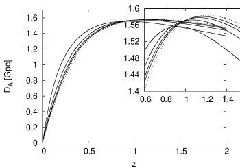
Figure 1: Angular diameter distance – redshift diagram for models with equation of state $P=K\rho$. The dashed curve has $K=0$, and the solid curves from the top to the bottom (at the maximum) have $K=0.0005$, $0.001$, $0.002$ and $0.005$.

Figure 2: Residual Hubble diagram for models with equation of state $P=K\rho$. The dashed curve has $K=0$, and the solid curves from the top to the bottom (at the maximum) have $K=0.005$, $0.002$, $0.001$ and $0.0005$.

It is apparent that for a linear equation of state, an increase in the proportionality constant, $K$, results in increasingly larger differences in the distance measurements (figures 1 and 2). For low redshifts, $z\lesssim 1$, the pressure-free Lemaître-Tolman model has smaller values of the distance at equal redshifts. Moreover as $K$ increases, so too does the value of the distance. This feature is better depicted in the residual Hubble diagram, figure 2, where the variation in magnitude as a function of redshift is large at small redshifts but becomes less distinguishable for $z\gtrsim 1$. Deviations from a linear equation of state are depicted in figures 3 and 4. In these figures we have only varied $n$ between $1.05$ and $0.95$, thereby indicating the sensitive nature of this parameter on the distance measurements. This is due to small variations in $n$ implying large variations in the magnitude of the pressure gradient with respect to the energy-density. Again, the residual Hubble diagram highlights the importance of this parameter at low redshifts, $z\lesssim 1$, where a variation of $n$ by $0.1$ can cause $\Delta m$ to vary by up to $0.6$.

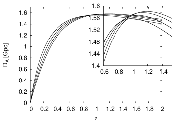
Figure 3: Angular diameter distance as a function of redshift for models with equation of state $P=10^{-3}\rho^{n}$. The curves from top to bottom (at the maximum) have $n=1.05$, $1.00$, $0.97$ and $0.95$.

Figure 4: Residual Hubble diagram for models with equation of state $P=10^{-3}\rho^{n}$. The curves from top to bottom (at the maximum) have $n=0.95$, $0.97$, $1.00$ and $1.05$.

Another interesting feature is that the position of the maximum of the angular diameter distance shifts to lower redshifts as the amplitude of the pressure gradient increases. As recently shown by Alfedeel & Hellaby (2009) the position of the apparent horizon (${\rm d}D_{A}/{\rm d}z=0$) for non-zero pressure models is given by the same relation as for the dust models, i.e. $R=2M$. However, since for $p^{\prime}\neq 0$ the function $M$ depends on time and thus this relation is satisfied by a different pair of $t$ and $r$ than in the dust models.

As can be seen from figures 1–4, the incorporation of pressure gradients in cosmological models can significantly alter the distance – redshift relations. For models with a positive pressure gradient, the luminosity distance for a given redshift is larger compared with models for $P=0$. It is therefore apparent that cosmological models with non-trivial pressure distributions will yield different results than cosmological models that do not consider pressure gradients.

5 Conclusion

Whilst a considerable amount of literature has been dedicated to the effect of inhomogeneous cosmological models to explain the observed distance – redshift relations from SN Ia data (Dabrowski & Hendry, 1998; Pascual-Sanchez, 1999; Célérier, 2000; Tomita, 2000, 2001a, 2001b; Iguchi et al., 2002; Godłowski et al., 2004; Alnes & Amarzguioui, 2006; Chung & Romano, 2006; Alnes & Amarzguioui, 2007; Enqvist & Mattsson, 2007; Alexander et al., 2007; Bolejko, 2008; Garcia-Bellido & Haugbøelle, 2008a, b; Zibin et al., 2008; Yoo et al., 2008; Enqvist, 2008; Bolejko & Wyithe, 2009; Célérier et al., 2009), surprisingly little has been done on the effect of pressure gradients in such models. The most simple invocation of pressure gradients into inhomogeneous cosmologies is to utilise spherically symmetric Lemaître models with an observer placed at the center of symmetry. In Bolejko & Lasky (2008), we studied these models to show that anomalous singularities that may occur in the evolution of such dust spacetimes (Hellaby & Lake, 1985; Bolejko et al., 2005) are delayed by the inclusion of realistic pressure gradients until significantly after structure formation has taken place. In the present article we have continued this line of research to derive the distance – redshift relations in spherically symmetric spacetimes endowed with a perfect fluid. Moreover, we worked in comoving coordinates with the observer at the center of symmetry. This work will therefore allow for an interpretation of cosmological data using such models.

By exploiting specific examples of inhomogeneous matter distributions with various “simple” equations of state, we have shown that the introduction of pressure gradients can have a non-negligble effect on observations, particularly for $z\lesssim 1$ (figures 1–4). This implies that one should definitely consider the full effect of pressure gradients in interpreting cosmological data-sets. However, this is a non-trivial task due to the increased number of free-parameters in the system. Indeed, if the data can be realistically fit using a void model with $P=0$, then it can equally well be fit by implementing slightly different matter distributions with $P\neq 0$. The problem then becomes one of reverse engineering the correct spacetime geometry from the numerous observations, a task which has been discussed in great detail in Lu & Hellaby (2007); McClure & Hellaby (2008).

We conclude by remarking that this work may also have a significant effect on interpretations of models with dark energy which is not a cosmological constant, but instead a dynamical field or negative pressure fluid (e.g. Basilakos, 2003; Linder & Jenkins, 2003; Linder, 2005; Kuhlen et al., 2005; Abramo et al., 2007, 2008; Mota et al., 2008; Avelino et al., 2008; Abramo et al., 2009). These models necessarily have inhomogeneous spacetime geometries, which is equally attributed to “pressure” gradients of the dark energy field. In this way, the distance – redshift relations that we have derived herein will be equally valid, and can therefore also be used to interpret cosmological data within such models.

References

- (1)
- Abramo et al. (2007) L. R. Abramo, et al. (2007). ‘Structure formation in the presence of dark energy perturbations’. J. Cosm. Astropart. Phys. 11:012.
- Abramo et al. (2008) L. R. Abramo, et al. (2008). ‘Dynamical mutation of dark energy’. Phys. Rev. D 77:067301.
- Abramo et al. (2009) L. R. Abramo, et al. (2009). ‘Physical approximations for the nonlinear evolution of perturbations in inhomogeneous dark energy scenarios’. Phys. Rev. D 79:023516.
- Alexander et al. (2007) S. Alexander, et al. (2007). ‘Local void vs dark energy: Confrontation with WMAP and Type Ia supernovae’. arXiv:0712.0370.
- Alfedeel & Hellaby (2009) A. A. H. Alfedeel & C. Hellaby (2009). ‘The Lemaitre model and the generalisation of the cosmic mass’. arXiv:0906.2343.
- Alnes & Amarzguioui (2006) H. Alnes & M. Amarzguioui (2006). ‘CMB anisotropies seen by an off-center observer in a spherically symmetric inhomogenous Universe’. Phys. Rev. D 74:103520.
- Alnes & Amarzguioui (2007) H. Alnes & M. Amarzguioui (2007). ‘Supernova Hubble diagram for off-center observers in a spherically symmetric inhomogeneous Universe’. Phys. Rev. D 75:023506.
- Avelino et al. (2008) P. P. Avelino, et al. (2008). ‘Clustering properties of dynamical dark energy models’. Phys. Rev. D 77:101302.
- Basilakos (2003) S. Basilakos (2003). ‘Cluster formation rate in models with dark energy’. Astrophys. J. 590:636.
- Biswas & Notari (2008) T. Biswas & A. Notari (2008). ‘’Swiss-cheese’ inhomogeneous cosmology and the dark energy problem’. J. Cosm. Astropart. Phys. 06:21.
- Bolejko (2006) K. Bolejko (2006). ‘Radiation in the process of the formation of voids’. Mon. Not. R. Astron. Soc. 370:924.
- Bolejko (2008) K. Bolejko (2008). ‘Supernova 1a observations in the Lemaître-Tolman model’. PMC Physics A 2:1.
- Bolejko (2009) K. Bolejko (2009). ‘The Szekeres swiss cheese model and the CMB observations’. Gen. Rel. Grav. 41:1737.
- Bolejko et al. (2005) K. Bolejko, et al. (2005). ‘Formation of voids in the Universe within the Lemaître-Tolman model’. Mon. Not. R. Astron. Soc. 362:213.
- Bolejko & Lasky (2008) K. Bolejko & P. D. Lasky (2008). ‘Pressure gradients, shell crossing singularities and acoustic oscillations - applications to inhomogeneous cosmological models’. Mon. Not. R. Astron. Soc. 391:L59.
- Bolejko & Wyithe (2009) K. Bolejko & J. S. B. Wyithe (2009). ‘Testing the Copernican principle via cosmological observations’. J. Cosm. Astropart. Phys. 2:20. arXiv:0807.2891.
- Brouzakis et al. (2007) N. Brouzakis, et al. (2007). ‘The effect of large scale inhomogeneities on the luminosity distance’. J. Cosm. Astropart. Phys. 7:02013.
- Brouzakis et al. (2008) N. Brouzakis, et al. (2008). ‘Light propagation and large-scale inhomogeneities’. J. Cosm. Astropart. Phys. 04:008.
- Caldwell & Stebbins (2008) R. R. Caldwell & A. Stebbins (2008). ‘A test of the Copernican principle’. Phys. Rev. Lett. 100:191302.
- Célérier et al. (2009) M. Célérier, et al. (2009). ‘A (giant) void is not mandatory to explain away dark energy with a Lemaitre – Tolman model’. arXiv:0906.0905.
- Célérier (2000) M.-N. Célérier (2000). ‘Do we really see a cosmological constant in the supernovae data?’. Astron. Astrophys. 353:63.
- Célérier (2007) M.-N. Célérier (2007). ‘The accelerated expansion of the Universe challenged by an effect of the inhomogeneities. A review’. New Adv. Phys. 1:29.
- Chung & Romano (2006) D. J. H. Chung & A. E. Romano (2006). ‘Mapping luminosity-redshift relationship to Lemaitre-Tolman-Bondi cosmology’. Phys. Rev. D 74:103507.
- Clarkson & Barrett (1999) C. Clarkson & R. K. Barrett (1999). ‘Does the isotropy of the CMB imply a homogeneous universe? Some generalized EGS theorems’. Class. Quantum Grav. 16:3781.
- Clarkson et al. (2008) C. Clarkson, et al. (2008). ‘A general test of the Copernican principle’. Phys. Rev. Lett. 101:011301.
- Clifton et al. (2008) T. Clifton, et al. (2008). ‘Living in a void: Testing the Copernican principle with distant supernovae’. Phys. Rev. Lett. 101:131302.
- Dabrowski et al. (2007) M. P. Dabrowski, et al. (2007). ‘How far is it to a sudden future singularity of pressure’. Phys. Rev. D 75:123524.
- Dabrowski & Hendry (1998) M. P. Dabrowski & M. A. Hendry (1998). ‘The Hubble diagram of type Ia supernovae in non-uniform pressure Universes’. Astrophys. J. 498:67.
- Ellis (2008) G. F. R. Ellis (2008). ‘Cosmology: Patchy solutions’. Nature 452:158.
- Ellis et al. (1985) G. F. R. Ellis, et al. (1985). ‘Ideal observational cosmology’. Phys. Rep. 124:315.
- Enqvist (2008) K. Enqvist (2008). ‘Lemaitre-Tolmans-Bondi model and accelerating expansion’. Gen. Rel. Grav. 40:451.
- Enqvist & Mattsson (2007) K. Enqvist & T. Mattsson (2007). ‘The effect of inhomogeneous expansion on the supernova observations’. J. Cosm. Astropart. Phys. 7:02019.
- Etherington (1933) I. M. H. Etherington (1933). ‘On the definition of distance in General Relativity’. Phil. Mag. ser. 7 15:761; reprinted in 2007, Gen. Rel. Grav., 39, 1055.
- February et al. (2009) S. February, et al. (2009). ‘Rendering dark energy void’. arXiv:0909.1479.
- Garcia-Bellido & Haugbøelle (2008a) J. Garcia-Bellido & T. Haugbøelle (2008a). ‘Confronting Lemaitre-Tolman-Bondi models with observational cosmology’. J. Cosm. Astropart. Phys. 4:3.
- Garcia-Bellido & Haugbøelle (2008b) J. Garcia-Bellido & T. Haugbøelle (2008b). ‘Looking the void in the eyes - the kinematic Sunyaev-Zeldovich effect in Lemaitre-Tolman-Bondi models’. J. Cosm. Astropart. Phys. 09:16.
- Garcia-Bellido & Haugbøelle (2009) J. Garcia-Bellido & T. Haugbøelle (2009). ‘The radial BAO scale and cosmic shear, a new observable for inhomogeneous cosmologies’. J. Cosm. Astropart. Phys. 9:28.
- Godłowski et al. (2004) W. Godłowski, et al. (2004). ‘Can the Stephani model be an alternative to FRW accelerating models?’. Class. Quantum Grav. 21:3953.
- Hellaby (2009) C. Hellaby (2009). ‘Modelling inhomogeneity in the Universe’. arXiv:0910.0350.
- Hellaby & Lake (1985) C. Hellaby & K. Lake (1985). ‘Shell crossings and the Tolman model’. Astrophys. J. 290:381.
- Hoyle & Vogeley (2004) F. Hoyle & M. S. Vogeley (2004). ‘Voids in the two-degree field galaxy redshift survey’. Astrophys. J. 607:751.
- Iguchi et al. (2002) H. Iguchi, et al. (2002). ‘Is dark energy the only solution to the apparent acceleration of the present Universe?’. Progr. Theor. Phys. 108:809.
- Jia & Zhang (2008) J. Jia & H. Zhang (2008). ‘Can the Copernican principle be tested by cosmic neutrino background?’. arXiv:0809.2597.
- Kolb et al. (2009) E. W. Kolb, et al. (2009). ‘Cosmological backgroun solutions and cosmological backreactions’. arXiv:0901.4566.
- Krasiński (1997) A. Krasiński (1997). Inhomogeneous cosmological models. Cambridge University Press, Cambridge.
- Kuhlen et al. (2005) M. Kuhlen, et al. (2005). ‘Dark energy and dark matter haloes’. Mon. Not. R. Astron. Soc. 357:387.
- Kwan et al. (2009) J. Kwan, et al. (2009). ‘Fractal bubble cosmology: A concordant cosmologcal model?’. arXiv:0902.4249.
- Lemaître (1933) G. Lemaître (1933). ‘L’univers en expansion’. Ann. Soc. Sci. Bruxelles A 53:51.
- Linder (2005) E. V. Linder (2005). ‘Cosmic growth history and expansion history’. Phys. Rev. D 72:043529.
- Linder & Jenkins (2003) E. V. Linder & A. Jenkins (2003). ‘Cosmic structure growth and dark energy’. Mon. Not. R. Astron. Soc. 346:573.
- Lu & Hellaby (2007) T. H.-C. Lu & C. Hellaby (2007). ‘Obtaining the spacetime metric from cosmological observations’. Class. Quantum Grav. 24:4107.
- Marra et al. (2007) V. Marra, et al. (2007). ‘Cosmological observables in a swiss-cheese Universe’. Phys. Rev. D 76:123004.
- McClure & Hellaby (2008) M. L. McClure & C. Hellaby (2008). ‘The metric of the cosmos II: Accuracy, stability, and consistency’. Phys. Rev. D 78:044005.
- Misner & Sharp (1964) C. W. Misner & D. H. Sharp (1964). ‘Relativistic equations for adiabatic, spherically symmetric gravitational collapse’. Phys. Rev. Lett. 136:B571.
- Moffat (2008) J. W. Moffat (2008). ‘Inhomogeneous cosmology, inflation and late-time accelerating universe’. arXiv:astro-ph/0606124.
- Mota et al. (2008) D. F. Mota, et al. (2008). ‘On the magnitude of dark energy voids and overdensities’. Astrophys. J. 675:29.
- Mustapha et al. (1998) N. Mustapha, et al. (1998). ‘The distortion of the area distance-redshift relation in inhomogeneous isotropic universes’. Class. Quantum Grav. 15:2363.
- Pascual-Sanchez (1999) J. F. Pascual-Sanchez (1999). ‘Cosmic acceleration: Inhomogeneity versus vacuum energy’. Mod. Phys. Lett. A 14:1539.
- Podurets (1964a) M. A. Podurets (1964a). ‘On one form of Einstein’s equations for a spherically symmetrical motion of a continuous medium’. Astronomicheskii Zhurnal 41:28.
- Podurets (1964b) M. A. Podurets (1964b). ‘On one form of Einstein’s equations for a spherically symmetrical motion of a continuous medium’. Soviet Astronomy 8:19.
- Stelmach & Jakacka (2006) J. Stelmach & I. Jakacka (2006). ‘Angular sizes in spherically symmetric Stephani cosmological models’. Class. Quantum Grav. 23:6621.
- Stoeger et al. (1992) W. R. Stoeger, et al. (1992). ‘Observational cosmology. V. Solution of the first-order general perturbation equations’. Class. Quantum Grav. 9:1725.
- Tolman (1934) R. C. Tolman (1934). ‘Effect of inhomogeneity on cosmological models’. Proc. Nat. Acad. Sci. USA 20:169–76.
- Tomita (2000) K. Tomita (2000). ‘Distances and lensing in cosmological void models’. Astrophys. J. 529:38.
- Tomita (2001a) K. Tomita (2001a). ‘A local void and the accelerating Universe’. Mon. Not. R. Astron. Soc. 326:287.
- Tomita (2001b) K. Tomita (2001b). ‘Analyses of type Ia supernova data in cosmological models with a local void’. Progr. Theor. Phys. 106:929.
- Uzan et al. (2008) J.-P. Uzan, et al. (2008). ‘Time drift of cosmological redshifts as a test of the Copernican principle’. Phys. Rev. Lett. 100:191303.
- Wiltshire (2007a) D. Wiltshire (2007a). ‘Cosmic clocks, cosmic variance and cosmic averages’. New J. Phys. 9:377.
- Wiltshire (2007b) D. Wiltshire (2007b). ‘Exact solution to the averaging problem in cosmology’. Phys. Rev. Lett. 99:251101.
- Wiltshire (2008) D. Wiltshire (2008). ‘Cosmological equivalence principle and the weak-field limit’. arXiv:0809.1183.
- Yoo et al. (2008) C. Yoo, et al. (2008). ‘Solving the inverse problem with inhomogeneous universes’. Progr. Theor. Phys. 120:937.
- Zibin et al. (2008) J. P. Zibin, et al. (2008). ‘Can we avoid dark energy?’. Phys. Rev. Lett. 101:251303.