Scattering Theory of Current-Induced Spin Polarization

Abstract

We construct a novel scattering theory to investigate magnetoelectrically induced spin polarizations. Local spin polarizations generated by electric currents passing through a spin-orbit coupled mesoscopic system are measured by an external probe. The electrochemical and spin-dependent chemical potentials on the probe are controllable and tuned to values ensuring that neither charge nor spin current flow between the system and the probe, on time-average. For the relevant case of a single-channel probe, we find that the resulting potentials are exactly independent of the transparency of the contact between the probe and the system. Assuming that spin relaxation processes are absent in the probe, we therefore identify the local spin-dependent potentials in the sample at the probe position, and hence the local current-induced spin polarization, with the spin-dependent potentials in the probe itself. The statistics of these local chemical potentials is calculated within random matrix theory. While they vanish on spatial and mesoscopic average, they exhibit large fluctuations, and we show that single systems typically have spin polarizations exceeding all known current-induced spin polarizations by a parametrically large factor. Our theory allows to calculate quantum correlations between spin polarizations inside the sample and spin currents flowing out of it. We show that these large polarizations correlate only weakly with spin currents in external leads, and that only a fraction of them can be converted into a spin current in the linear regime of transport, which is consistent with the mesoscopic universality of spin conductance fluctuations. We numerically confirm the theory.

I Introduction

I.1 Electric generation of spin polarization

Two purely electric mechanisms have been proposed to generate spin accumulations in electronic systems with spin-orbit interaction (SOI). They are current-induced spin polarization cisp ; Ede90 and the spin Hall effect Dya71a ; she . Both phenomena appear when a spin-orbit coupled conductor is traversed by an electric current. Current-induced spin polarization manifests itself in a weak bulk polarization of the electronic spins in a direction determined by the electric current and the SOI, while the spin Hall effect manifests itself in a spin accumulation at the lateral edges of the sample. Though the resulting polarizations are usually rather weak, both effects have been demonstrated experimentally Kat04 ; Wun05 ; Val06 ; Sai06 ; Zha06 . They offer an elegant alternative to spin injection and manipulation with ferromagnets, Zeeman fields or by optical means, and pave the way toward spintronic devices with purely electric control of electronic spins.

A dual aspect of these magnetoelectric effects is that they are accompanied by spin currents, flowing either inside the sample or leaving it. Early analytical investigations of these spin currents have been devoted to calculations of bulk spin conductivities, but it was soon realized that the latter are not always related to physically relevant quantities. Local approaches based on classical kinetic equations have been used to investigate the conversion of magnetoelectric spin accumulations at the edge of a spin-orbit coupled sample into spin currents leaving the sample she ; Mis04 ; Bur04 ; Mal05 ; Ada07 ; Tserk . These quasiclassical theories have been quite successful, however they neglect coherent effects and, in their present form, are not appropriate to investigate local fluctuations and spatial correlations of spin polarization. Coherent mesoscopic effects on spin currents have recently attracted quite some theoretical attention, both analytically Cha05 ; Bar07 ; Naz07 ; Kri08 ; Ada09 ; Kri09 and numerically Nik05 ; guo , in both diffusive and ballistic systems, while so far only mesoscopic fluctuations of sample-integrated spin polarizations in the diffusive regime have been investigated Duc08 . At present, little is known about local coherent fluctuations of spin polarizations, the scale on which they occur, how they are correlated, and how they influence spin currents and their fluctuations, neither have current-induced spin polarizations in chaotic ballistic systems been investigated so far. It is the purpose of this article to start filling these gaps, by investigating the magnetoelectric generation of spin polarizations in ballistic mesoscopic samples.

To that end we construct a spin-probe model, which connects local spin-dependent chemical potentials to those imposed on a nearby probe. In this way, we are able to express local current-induced spin polarizations in terms of transmission coefficients deriving from the scattering matrix. Focusing on chaotic ballistic mesoscopic systems, we then use random matrix theory  Bro96 ; mehta to calculate the statistics of these polarizations. We find that, while the ensemble average polarization vanishes, it fluctuates from position to position (in a given sample) and from sample to sample. For sufficiently large systems, the amplitude of these fluctuations by far exceeds the magnitude of all current-induced polarizations investigated to date. Simultaneously, we show that this polarization is mostly uncorrelated with spin currents in external leads and thus cannot easily be converted into a large spin current, at least not in linear response.

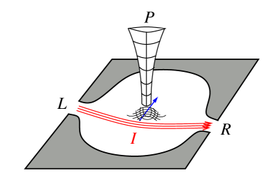
Figure 1: The spin-probe set-up. An open quantum dot with spin-orbit interaction is traversed by an electric current ($I$). The magnetoelectrically generated spin accumulation is measured locally by an external probe ($P$) where spin-orbit interaction is absent. The charge and spin-resolved electrochemical potentials of the probe are set such that no spin nor charge current flow between the dot and the probe. When the probe is contacted to the system via a tunnel barrier of low transparency, we argue that the spin-dependent potentials in the probe can be identified with the local spin-resolved potentials in the sample at the contact with the probe. This allows to relate spin accumulations to spin-dependent transmission coefficients.

I.2 The spin-probe model

Fig. 1 gives a sketch of the system we focus on. We consider a two-dimensional chaotic ballistic quantum dot connected via reflectionless transport terminals to two external electron reservoirs. The reservoirs are biased and an electric current flows through the dot. Assuming that SOI is strong enough that the spin-orbit time is shorter than the mean electronic dwell time in the dot, $\tau_{\rm so}\ll\tau_{\rm D}$, spin rotational symmetry is totally broken inside the dot. Together with chaotic boundary scattering, this leads to spin relaxation. Does the current flowing through this SOI coupled, spin-relaxing system generate a spin polarization ? On one hand, the relative positions of the contacts to the external electrodes determine an average electronic drift. In that sense, the situation is very similar to that considered by Edelstein Ede90 , and one would accordingly argue that a current-induced spin polarization should emerge. On the other hand, however, electronic distribution functions are not well defined locally in such a system where momentum and energy relax on the scale of the system itself. One might thus wonder how local spin-dependent potentials can be consistently defined.

Here, we circumvent this difficulty by introducing an additional mobile terminal whose purpose it is to probe the local chemical potentials on the dot. We assume that spin currents are well defined in the probe as well as in the transport terminals, which presupposes that spin relaxation processes are frozen there. In particular, SOI is present only in the dot. The probe is assumed to carry a single-transport channel. It is connected at one end to a macroscopic external reservoir, which defines its electrochemical and spin-dependent chemical potentials unambiguously, while its other end is contacted to the quantum dot via a tunnel barrier of transparency $0\leq\Gamma_{P}\leq 1$. When $\Gamma_{P}\ll 1$, the probe does not perturb the dot and we can identify the spin-dependent chemical potentials on the dot with the corresponding probe potentials defined by the condition that neither charge nor spin currents flow between the probe and the dot caveat1 . The probe being mobile, it can scan the whole dot area, and being single-channeled, it has maximal resolution. It can thus map the spin-polarization in the dot with maximal accuracy.

I.3 Summary of main results

The spin-probe model becomes a powerful theoretical tool to calculate spin accumulations once electric and spin currents in the probe and the two transport terminals are related to chemical potentials via the scattering approach to transport But86 ; Imr86 . When the probe carries a single transport channel, time-reversal symmetry and the unitarity of the scattering matrix ensure that the reflection coefficients from the probe back to itself are diagonal in spin indices, independently of $\Gamma_{P}$. This allows to directly express the electrochemical and spin-dependent chemical potentials of the probe in terms of spin-dependent transmission coefficients from the transport leads to the probe, and the chemical potentials at those leads. This is done below in Eq. (9). We additionally find that, for a single-channel probe, the dependence that transmission coefficients have on $\Gamma_{P}$ factorizes. This has the important, and somewhat surprising consequence that the chemical potentials ensuring the vanishing of the currents through the probe, being given by the ratio of transmission coefficients, do not depend on $\Gamma_{P}$. This is an exact result, valid as long as one has a single-channel probe, and we stress that it is true not only on average nor to some leading order. Consequently, we are able to obtain the value of the spin-dependent potentials on the probe in the limit $\Gamma_{P}\rightarrow 0$, where it is justified to identify the potentials on the dot with those on the probe, while performing the calculation for the analytically simpler case $\Gamma_{P}=1$.

Our scattering theory of spin accumulations can be applied to both diffusive and ballistic mesoscopic systems in the linear response regime. Because current-induced spin polarization has not been considered in these systems so far, we specialize here to ballistic systems, and accordingly apply random matrix theory (RMT) Bro96 ; mehta to calculate average and fluctuations of the spin-resolved local chemical potentials. We perform our calculation for $\Gamma_{P}=1$ to avoid unnecessary complications arising from the presence of a Poisson kernel for $\Gamma_{P}<1$ Bro96 . We find that, within RMT, there is no current-induced local spin polarization on mesoscopic average. However, sample-dependent or probe position-dependent fluctuations make local spin-dependent chemical potentials fluctuate with a variance

$${\rm var}\,\mu_{P}^{(\beta)}\simeq\frac{(eV)^{2}}{32N}\,,$$ (1)

given by the voltage bias $V$ between the two transport leads and the number $N$ of channels each of them carries. The above formula gives the leading order contribution in $1/N\ll 1$. The exact formula is given below in Eq. (14). Within RMT, the variance is the same for $\beta=x,y$ and $z$.

The transmission coefficients from the transport terminals to the probe are elements of a scattering matrix which depends on the position of the probe. Therefore, as the probe scans the sample, these coefficients fluctuate. Below, we conjecture and numerically confirm that, within RMT, moving a single-channel terminal by a single Fermi wavelength is sufficient to decorrelate transmission coefficients to and from that terminal. This has for consequence that the total polarization integrated over the entire dot, while still averaging to zero, acquires a sample-to-sample variance given by the single-channel local variance multiplied by the total number $k_{\rm F}^{2}A/4\pi$ of uncorrelated probe positions. Thus,

$${\rm var}\,\mu_{\rm tot}^{(\beta)}\simeq\frac{k_{\rm F}^{2}A}{4\pi}\,\frac{(eV)^{2}}{32N}\,.$$ (2)

Because $\mu_{\rm tot}^{(\beta)}$ gives the chemical potential difference between the two possible spin orientation along the spin axis $\beta=x,y,z$, dividing it by twice the level spacing converts it into a number of polarized spins in that direction. This gives the typical number of polarized spins in a given sample as

$$\langle S^{(\beta)}_{\rm typ}\rangle=\frac{{\rm rms}\,\mu_{\rm tot}^{(\beta)}}{2\delta}\simeq\frac{C}{16}\,\sqrt{\frac{k_{\rm F}L^{2}}{2W}}\,\frac{eV}{\delta}\,,$$ (3)

with the dot level spacing $\delta=2\pi/mA$, the width $W$ of the transport terminals and the linear dot size $L$. Eq. (3) is one of our main results. It predicts that linear electric transport across a typical, ballistic mesoscopic quantum dot generates a giant polarization of the electronic spins inside the dot in the semiclassical limit $k_{\rm F}L\gg 1$, and for a large enough dwell time $L/W\gg 1$. This typical polarization is in particular much larger than the average magnetoelectric polarization predicted by Edelstein Ede90

$$\langle S^{(\rm E)}\rangle=4\frac{k_{\alpha}\ell}{k_{\rm F}L}\,\frac{eV}{\delta}\,,$$ (4)

in a diffusive dot with elastic mean free path $\ell\ll L$ and with Rashba SOI whose strength $k_{\alpha}$ is usually only a fraction of $k_{\rm F}$. It is also much larger than the typical Duckheim-Loss polarization Duc08 ,

$$\langle S^{(\rm DL)}_{\rm typ}\rangle\propto\frac{1}{k_{\rm F}\ell\,k_{\alpha}L}\,\frac{eV}{\delta}\,,$$ (5)

predicted for $k_{\alpha}L\gg 1$. Despite its magnitude, $\langle S^{(\beta)}_{\rm typ}\rangle$ cannot easily be converted into a large spin current. Below we demonstrate this by calculating the correlator of the spin polarization with the spin current in external leads, and show that this correlator vanishes unless the probe is within a Fermi wavelength of the contact to the terminal. In other words, RMT predicts that only accumulations right at the boundary of the sample can be extracted and converted into spin currents in the linear regime, which is consistant with the universal fluctuations of spin currents found in Refs. Bar07 ; Naz07 ; Kri08 ; Ada09 . It is at present unclear if more spin current can be extracted in nonlinear regimes of transport.

Having summarized our method and main findings, we now proceed to present our theory more formally. In the next Section II, we construct a scattering theory of current-induced spin polarization. In Section III, we focus on ballistic systems and apply RMT to calculate the mean and variance of the local as well as of the sample-integrated polarizations. We further demonstrate the power of our approach by calculating correlators of spin polarizations with spin currents. Section IV is devoted to a numerical proof-of-principle of our theory and a quantitative confirmation of our main result, Eq. (3). We conclude with a brief discussion of our results and of future challenges and demonstrate the $\Gamma_{P}$-independence of the probe voltages for $N_{P}=1$ in an appendix.

II Scattering theory of current-induced spin polarization

In its standard form, the scattering approach to transport gives a linear relation between currents and voltages measured in external leads But86 ; Imr86 . It applies equally well to diffusive and ballistic systems. Extended to take account of spin currents and chemical potentials in a multiterminal geometry, the relation reads

$$I_{i}^{(\alpha)}=\frac{e}{h}\sum_{j,\beta}(2N_{i}\Gamma_{i}\delta_{\alpha\beta}\delta_{ij}-\mathcal{T}^{(\alpha\beta)}_{ij})\mu_{j}^{(\beta)}\,,$$ (6)

where Greek letters label spin indices and Latin letters label electric terminals. Here, $N_{i}$ gives the number of transport channels in terminal $i$, $\Gamma_{i}$ the transparency of the contact between that terminal and the dot, $\mu_{i}^{(0)}=E_{\rm F}+eV_{i}$ gives the electrochemical potential in terms of the Fermi energy $E_{\rm F}$ and the applied voltage $V_{i}$, and $\mu_{i}^{(\beta)}$ give the chemical potential difference between the two possible spin orientation along the spin axis $\beta=x,y,z$ caveat2 . We further defined $I^{(0)}_{i}\equiv I_{i}$ and $I_{i}^{(\alpha)}$ as the charge current and the three components of the spin current vector respectively, and introduced the spin-dependent transmission coefficients Ada09

$$\mathcal{T}_{ij}^{(\alpha\beta)}=\sum_{m\in i,n\in j}{\rm Tr}[t_{mn}^{\dagger}\sigma^{\alpha}t_{mn}\sigma^{\beta}],$$ (7)

where $\sigma^{\alpha}$, $\alpha=x,y,z$ are Pauli matrices and $\sigma^{0}$ is the identity matrix. The trace in Eq. (7) is taken over the spin degree of freedom and $t_{mn}$ is a 2$\times$2 matrix of spin-dependent transmission amplitudes from channel $n$ in lead $j$ to channel $m$ in lead $i$.

We are interested in the mesoscopic counterpart of the magnetoelectric geometry of Ref. Ede90 , and consider a quantum dot connected to two external transport terminals $L$ and $R$. An electric bias voltage $V$ is applied between the terminals, $\mu_{L}^{(0)}-E_{\rm F}=-\mu_{R}^{(0)}+E_{\rm F}=eV/2$, where we further assume that there is no spin accumulation, $\mu_{L,R}^{(\beta)}=0$, $\beta\neq 0$. To measure local chemical potentials, we introduce an external probe with controllable chemical potentials, which scans the dot surface. The situation is sketched in Fig. 1. The chemical potentials in the probe are determined by the condition that no charge nor spin current flows through it, i.e. they are solutions of

$$I_{P}^{(\alpha)}=\frac{e}{h}\sum_{j=L,R,P}\sum_{\beta}(2\Gamma_{P}N_{P}\delta_{\alpha\beta}\delta_{{\rm P},j}-\mathcal{T}^{(\alpha\beta)}_{{\rm P},j})\mu_{j}^{(\beta)}\equiv 0\,,$$ (8)

and depend a priori on the transparency of the contact between the probe and the dot. Eq. (8) determines the local chemical potentials $\mu_{P}^{(\beta)}$ as a function of the electrochemical potentials $\mu_{L,R}^{(0)}$ imposed on the longitudinal leads. We consider a single-channel probe $N_{\rm P}=1$, which not only delivers the sharpest resolution of the dot’s chemical potentials landscape, but moreover ensures that the spin reflection matrix $\mathcal{T}_{PP}^{(\alpha\beta)}$ from the probe to itself is exactly (i.e. not only on average) diagonal in spin indices. This follows from time-reversal symmetry, current conservation and gauge invariance symmetry_gs0 , which additionally require $\mathcal{T}_{PP}^{(\alpha\alpha)}=\mathcal{T}_{PP}^{(00)}$, $\forall\alpha$. One then straightforwardly obtains the chemical potentials in the probe as

$$\mu_{P}^{(\beta)}=[\mathcal{T}^{(\beta 0)}_{PL}-\mathcal{T}^{(\beta 0)}_{PR}]eV\Big{/}2[\mathcal{T}^{(00)}_{PL}+\mathcal{T}^{(00)}_{PR}].$$ (9)

In particular, for $N_{L,R}\gg 1$, the electrochemical potential in the probe is given by

$$\mu_{\rm P}^{(0)}=[\mathcal{T}^{(00)}_{PL}-\mathcal{T}^{(00)}_{PR}]eV\Big{/}4\Gamma_{P}\,,$$ (10)

which reproduces a result first derived in Ref. But89 . In diffusive samples, this gives a linear average decay of $\mu_{P}^{(0)}$ from $eV/2$ to $-eV/2$ as the probe is moved across the sample from regions more easily accessible from the left lead (where $\mathcal{T}^{(00)}_{PL}>\mathcal{T}^{(00)}_{PR}$) to regions which are more easily accessible from the right.

We next make the key observation that the $\Gamma_{P}$-dependence of the transmission coefficients $\mathcal{T}^{(\alpha\beta)}_{PI}$ between the probe and the transport terminals $I=L,R$ exactly factorizes when the probe is single-channeled. This remarkable property is apparently mentioned here for the first time and is discussed in some detail in Appendix A. Consequently, the chemical potentials in Eq. (9) remain the same, regardless of the transparency of the tunnel barrier between the dot and the probe, when the latter carries only a single channel. Our aim being to obtain the current-induced spin polarization and thus the spin-dependent chemical potentials on the dot, we are quite naturally interested in the limit $\Gamma\rightarrow 0$, where the probe does not perturb the dot and accordingly the spin-dependent chemical potentials on the dot equal those on the probe. The observation we just made allows us to access that limit via an analytically simpler calculation at $\Gamma_{P}=1$ which we present in the next section.

To get the total spin polarization, we scan the probe over the whole sample. The transmission amplitudes $t_{mn}$ in Eq. (7) are elements of a scattering matrix that depends parametrically on the probe position. For a wide probe, $N_{P}\gg 1$, we argue semiclassically that the correlator $\langle\mathcal{T}^{(\alpha\beta)}_{PL}\mathcal{T}^{(\alpha\beta)}_{P^{\prime}L}\rangle-\langle\mathcal{T}^{(\alpha\beta)}_{PL}\rangle\langle\mathcal{T}^{(\alpha\beta)}_{P^{\prime}L}\rangle$ decays to zero when the distance between $P$ and $P^{\prime}$ is of order the width of the probe. This is so, because beyond that, correlated escapes of pairs of trajectories no longer contribute Jac06 . We next make the leap of faith that this semiclassical argument can be extended to the case of present interest of a single-channel probe, for which we accordingly conjecture that two measurements performed a distance $\sim k_{\rm F}^{-1}$ apart deliver uncorrelated outcomes. To the best of our knowledge, this problem has not been investigated yet, and we will numerically confirm the validity of this conjecture below. Further assuming a sharp decay of the correlator at $k_{\rm F}^{-1}$, we obtain that the sample-integrated chemical potentials are given by the sum $\mu_{\rm tot}^{(\beta)}=\sum_{P}\mu_{P}^{(\beta)}$ over $k_{\rm F}^{2}A/4\pi$ uncorrelated probe positions on the surface of our two-dimensional quantum dot.

III Random Matrix Theory

Having expressed local and sample-integrated polarizations in terms of transmission coefficients, Eq. (9), we next proceed to evaluate them quantitatively. We focus on ballistic chaotic cavities, and accordingly use RMT to calculate the average and variance of $\mu_{P}^{(\beta)}$ and $\mu_{\rm tot}^{(\beta)}$. This calculation is easier for $\Gamma_{P}=1$, since then the ensemble-average scattering matrix vanishes Bro96 . Because of the factorization property of the $\Gamma_{P}$-dependence of transmission coefficients mentioned above, the spin-dependent potentials on the dot are equal to those on the probe for $\Gamma_{P}\rightarrow 0$, which in their turn remain unchanged as $\Gamma_{P}\rightarrow 1$. Thus we can extract the dot’s spin-dependent potentials $\mu_{x_{P}}^{(\beta)}$ at point $x_{P}$ underneath the probe from a calculation at $\Gamma_{P}=1$, because $\mu_{x_{P}}^{(\beta)}=\mu_{P}^{(\beta)}(\Gamma_{P}\rightarrow 0)=\mu_{P}^{(\beta)}(\Gamma_{P}=1)$. Because we are interested in systems with time reversal symmetry but totally broken spin rotational symmetry, we take the scattering matrix as an element of the circular symplectic ensemble of random matrices mehta . RMT does not depend on the exact form of SOI, but only requires that SOI totally breaks spin rotational symmetry. Our results are thus expected to apply for Rashba and Dresselhaus SOI equally well, as long as one has a ballistic chaotic quantum dot with totally broken spin rotational symmetry.

For $N_{P}=1$, we get from Ref. Ada09

$$\langle\mathcal{T}_{ij}^{(\alpha\beta)}\rangle_{\rm RMT}=\frac{2\delta_{\alpha\beta}\,[N_{i}N_{j}\delta_{\alpha 0}-(\delta_{\alpha 0}-1/2)N_{i}\delta_{ij}]}{N_{L}+N_{R}+1/2}\,,$$ (11)

from which we conclude, together with Eq. (9), that

$$\langle\mu_{P}^{(\beta)}\rangle_{\rm RMT} = \langle\mu_{\rm tot}^{(\beta)}\rangle_{\rm RMT}=0\,.$$ (12)

RMT thus predicts the vanishing of the spin polarization on average. The latter is understood in the standard mesoscopic sense, as an average over changes in the dot shape, the overall chemical potential or the position of the leads.

Chemical potentials nevertheless exhibit spatial fluctuations in a single sample, whose magnitude can be estimated by calculating ${\rm var}\,\mu_{P}^{(\beta)}$. Of further interest are also mesoscopic fluctuations of the sample-integrated chemical potentials whose magnitude we analyze with ${\rm var}\,\mu_{\rm tot}^{(\beta)}$. To calculate the variance of $\mu_{P}^{(\beta)}$ in Eq. (9), we take the variance of the numerator and divide it by the squared average of the denominator, a procedure which neglects subdominant corrections ${\cal O}(N_{L,R}^{-1})$. The variance of the spin-dependent transmission coefficients have been calculated in Ref. Bar07 . For $i=L,R$, we have

$${\rm var}\mathcal{T}^{(\beta 0)}_{Pi}=\frac{4[N_{P}N_{i}(N_{\rm T}-1)-N_{P}N_{i}^{2}]}{N_{\rm T}(2N_{\rm T}-1)(2N_{\rm T}-3)}\,,$$ (13a)

$${\rm covar}(\mathcal{T}^{(\beta 0)}_{PL},\mathcal{T}^{(\beta 0)}_{PR})=\frac{-4N_{P}N_{L}N_{R}}{N_{\rm T}(2N_{\rm T}-1)(2N_{\rm T}-3)}\,,$$ (13b)

with $N_{\rm T}=N_{L}+N_{R}+N_{P}$. For our case with $N_{P}=1$, we obtain

$${\rm var}\,\mu_{P}^{(\beta)} = 16\,\left(\frac{eV}{4}\right)^{2}\frac{N_{L}N_{R}}{N_{\rm T}(2N_{\rm T}-1)(2N_{\rm T}-3)}\,.\qquad$$ (14)

For $N_{L}=N_{R}\equiv N\gg 1$, Eq. (14) goes into Eq.(1).

With the further assumptions, discussed in the previous section, that (i) spin relaxation processes are frozen in the probe and (ii) the correlator $\langle\mathcal{T}^{(\alpha\beta)}_{PL}\mathcal{T}^{(\alpha\beta)}_{P^{\prime}L}\rangle-\langle\mathcal{T}^{(\alpha\beta)}_{PL}\rangle\langle\mathcal{T}^{(\alpha\beta)}_{P^{\prime}L}\rangle$ sharply decays when the distance between the probe positions $P$ and $P^{\prime}$ reaches the Fermi wavelength, we get the typical total spin-dependent chemical potentials

$${\rm var}\,\mu_{\rm tot}^{(\beta)}=\frac{k_{\rm F}^{2}A}{4\pi}{\rm var}\,\mu_{P}^{(\beta)}\,.$$ (15)

As justified above, we identify these potentials with those on the dot. Assuming that they are generated by a spin polarization, we convert them into the variance of the spin polarization by dividing them with $2\delta$. For $N_{L}=N_{R}\equiv N$, we obtain the variance of the total number of polarized spins on the dot as

$${\rm var}\,S_{\rm dot}^{(\beta)}=\frac{k_{\rm F}^{2}A}{4\pi}\left(\frac{eV}{2\delta}\right)^{2}\frac{N^{2}}{(2N+1)(4N+1)(4N-1)}$$ (16)

which, for $N\rightarrow\infty$, gives Eq. (3). The validity of Eqs. (14–15) is numerically confirmed below in Fig. 3.

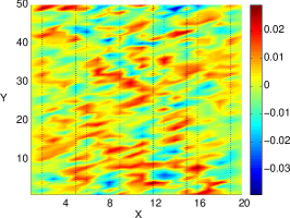
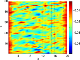
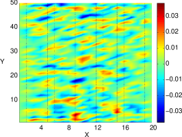
Figure 2: Numerical proof-of-principle for the local measurement of spin accumulations on a single, diffusive, Rashba-coupled lattice of size 20 $\times$ 50 traversed by an electric current in the positive $x$-direction (from left to right). The on-site disorder and Rashba spin-orbit interaction correspond to a mean free path $\ell=6a$ and a spin-orbit length $l_{\rm so}=9a$. The system has hard-wall boundary conditions at its top and bottom boundaries. From left to right, spin accumulations $\mu^{(\beta)}$ with $\beta=x$, $y$ and $z$. Only $\mu^{(y)}$ displays a finite average magnetoelectric effect (central panel), as predicted in Ref. Ede90 . Fluctuations exist for all spin orientations. The color scale is in units of the voltage bias $eV$. Note the different color scales in different panels.

The power of our scattering theory is perhaps even more evident when one realizes that it allows to calculate correlation functions between local spin polarizations inside the sample and spin currents in the leads. The spin current in lead $L$ is given by

$$I_{L}^{(\alpha)}=\frac{e^{2}V}{h}[\mathcal{T}_{LR}^{(\alpha 0)}-\mathcal{T}_{LL}^{(\alpha 0)}]-\frac{e}{h}\sum_{\beta}\mathcal{T}_{LP}^{(\alpha\beta)}\mu_{P}^{(\beta)}\,,$$ (17)

and each of these three terms gives a separate contribution to the correlator $\langle I_{L}^{(\alpha)}\mu_{P}^{(\beta)}\rangle-\langle I_{L}^{(\alpha)}\rangle\langle\mu_{P}^{(\beta)}\rangle$. For $\alpha=x,y,z$, the contribution of the third term vanishes because it contains the average of three spin-dependent transmission coefficients. Furthermore, RMT gives ${\rm covar}(\mathcal{T}^{(\alpha 0)}_{Pi},\mathcal{T}^{(\beta 0)}_{jk})\propto\delta_{ik}\delta_{\alpha\beta}\delta_{\alpha 0}$ if $j\neq P$. Therefore, for $\alpha=x,y,z$, the first two terms do not contribute either, unless the probe is placed in the immediate vicinity, i.e. within a single Fermi wavelength of the contact to the $L$ lead. In this case, nonvanishing covariances appear in $\langle\langle I_{L}^{(\alpha)}\mu_{P}^{(\beta)}\rangle\rangle$, see Eq. (13b), and one obtains

$$\langle\langle I_{L}^{(\alpha)}\mu_{P}^{(\beta)}\rangle\rangle=\frac{-8\,\delta_{\alpha\beta}\delta_{Px_{L}}\,N_{L}N_{R}}{N_{T}(2N_{T}-1)(2N_{T}-3)}\frac{e^{3}V^{2}}{h}\,,$$ (18)

where $\delta_{Px_{L}}$ requires that the probe be placed within $k_{\rm F}^{-1}$ of the boundary between the SOI-coupled dot and the lead. Summing over all possible probe positions, one obtains a universal correlator $\langle\langle I_{L}^{(\alpha)}\mu_{\rm tot}^{(\beta)}\rangle\rangle={\cal O}(N^{0})$ for $N_{L,R}\sim N\gg 1$, which is consistent with the universality of spin currents fluctuations Bar07 ; Naz07 ; Kri08 ; Ada09 . RMT thus predicts that coherent polarizations correlate with the spin currents only if they are right at the sample exit.

IV Numerics

We numerically illustrate the validity of our scattering theory of spin polarizations and confirm our main prediction, Eqs. (14-15). We use tight-binding models defined by the Hamiltonian

$${\cal H}=\sum_{i,j}\sum_{\alpha,s,s^{\prime}}h^{(\alpha)}_{ij}\sigma^{\alpha}_{s,s^{\prime}}c^{\dagger}_{is}c_{js^{\prime}}\,,$$ (19)

where the operators $c_{is}^{\dagger}$ ($c_{is}$) create (destroy) a spin-$1/2$ fermion with spin $s=\uparrow,\downarrow$ and $\sigma^{\alpha}_{s,s^{\prime}}$ indicate elements of Pauli matrices. To give a proof-of-principle for our approach, we consider a diffusive model, while quantitative confirmations of our theory are solely based on the RMT model.

For the diffusive model, $i=(i_{x},i_{y})$ labels a site on a two-dimensional lattice of size $L_{x}\times L_{y}=(N_{x}a)\times(N_{y}a)$ with spacing $a$, giving the size $M=N_{x}\times N_{y}$ of the Hamiltonian matrix. We further take $h^{(\alpha)}_{ij}=it_{\rm so}\delta_{\alpha,x}\delta_{i_{x},j_{x}}(\delta_{i_{y}+a,j_{y}}+\delta_{i_{y}-a,j_{y}})-it_{\rm so}\delta_{\alpha,y}\delta_{i_{y},j_{y}}(\delta_{i_{x}+a,j_{x}}+\delta_{i_{x}-a,j_{x}})-t\delta_{\alpha,0}[\delta_{i_{x},j_{x}}(\delta_{i_{y}+a,j_{y}}+\delta_{i_{y}-a,j_{y}})+\delta_{i_{y},j_{y}}(\delta_{i_{x}+a,j_{x}}+\delta_{i_{x}-a,j_{x}})]+w_{i}\delta_{\alpha,0}\delta_{i,j}$, corresponding to an on-site disorder potential with randomly distributed $w_{i}\in[-w/2,w/2]$, a nearest-neighbor hopping $t$ and a Rashba spin-orbit interaction $t_{\rm so}$. These parameters give a spin-orbit length $\ell_{\rm so}\approx\pi at/t_{\rm so}$ and an elastic mean free path $\ell\approx 48at^{2}/w^{2}$ close to half filling.

For the RMT model, we take $\sum_{\alpha}h^{(\alpha)}_{ij}\sigma^{\alpha}$ to be randomly distributed quaternions Bro96 ; mehta , with time-reversal symmetry requiring $h^{(0)}_{ij}=h^{(0)}_{ji}$, and $h^{(\alpha)}_{ij}=-h^{(\alpha)}_{ji}$ for $\alpha=x,y,z$. Generally, the indices $i,j$ have no particular physical meaning in RMT and the size $M$ of the Hamiltonian matrix is a free parameter. Here we attach the system to external leads, and also consider $i$ and $j$ to label sites on a two-dimensional lattice whose Hamiltonian has an infinite-range random hopping. Once the sharp decay of spin-spin correlations is confirmed, $M=k_{\rm F}^{2}A/4\pi$ gives the total number of uncorrelated probe positions. For both models, all our simulations fix the Fermi energy slightly below half-filling.

To construct the scattering matrix, we follow the method of Ref. Heidelberg . We introduce a $M\times N_{\rm T}$ projection matrix $W$ which connects the system to external leads. This matrix has only one nonzero element per row, at a spot determined by the coupling between the system and the leads. For an ideal contact, all nonzero matrix elements of $W$ are unity. The $N_{\rm T}\times N_{\rm T}$ scattering matrix ${\cal S}$ associated with ${\cal H}$ is given by

$${\cal S}=1-2\pi iW^{\dagger}(E_{\rm F}-{\cal H}+i\pi WW^{\dagger})^{-1}W\,,$$ (20)

with the overall Fermi energy $E_{\rm F}$. The transmission coefficients of Eq. (7) are straightforwardly obtained from ${\cal S}$. For the diffusive model, this method is certainly not the most efficient numerically. We still rely on it, because for the RMT model, the infinite-range hopping renders the implementation of recursive Green’s function algorithms problematic. Note that it is necessary to first generate random Hamiltonians from which random scattering matrices are constructed in order to consistently define probe positions and investigate whether spin-spin correlations decay sharply beyond a Fermi wavelength. To investigate the decay of these correlations, we generate a random ${\cal H}$ and take

$$W = \left(\begin{array}[]{ccc}{\mathbb{I}}_{N_{L}}&0&0\\ 0&\vec{v}_{M-N_{L}-N_{R}}&0\\ 0&0&{\mathbb{I}}_{N_{R}}\end{array}\right)\,,$$ (24)

where for each choice of $W$, only a single component of the column vector $\vec{v}$ (whose index indicates its length) is nonzero and equal to one. The position of that nonzero component determines the position of the probe on the two-dimensional lattice. Our Hamiltonians are defined on rectangular two-dimensional lattices, and we contact the transport modes at two of its edges, which is represented by the two identity matrices in Eq. (24).

We first show numerical proof-of-principle for the spin-probe mode. In Fig. 2, we present data for the local spin polarizations $\mu_{P}^{(\beta)}$, $\beta=x,y,z$. The three panels clearly show that, for transport in the $x$-direction and a Rashba SOI, there is a finite average magnetoelectrically induced polarization along the $y$-axis only, as predicted in Ref. Ede90 . Furthermore, there are local (as well as sample-to-sample) fluctuations of the spin polarization in all directions, as predicted in Ref. Duc08 . All accumulations vanish on average in the RMT model, moreover spatial fluctuations occur on the smallest possible scale of a single site, as expected, and we therefore do not show them here.

We next confirm our conjecture of a sharp decay of correlations, and to that end, we calculate the spin-spin correlation function $D(n)=\langle S^{(\beta)}(i)S^{(\beta)}(i+na\vec{e})\rangle$. For both diffusive as well as RMT models we found no significant anisotropy, i.e. $D$ was the same for $\vec{e}$ in the $x$ or $y$ direction. This is of course expected for the RMT model, but would deserve some more investigations in the diffusive case. The Fermi wavelength being equal to the lattice spacing close to half filling, one expects $D(n)=\delta_{n0}$ for the RMT model. This is confirmed in the inset of Fig. 3, where we additionally see that $D(n)$ is also sharply peaked at $n=0$ in the diffusive model, with some correlation persisting over few, $\sim$2-3 sites. This sharp decay of $D(n)$ in the diffusive model suggests that our conjecture of a fast decay of the correlator $\langle\mathcal{T}^{(\alpha\beta)}_{PL}\mathcal{T}^{(\alpha\beta)}_{P^{\prime}L}\rangle-\langle\mathcal{T}^{(\alpha\beta)}_{PL}\rangle\langle\mathcal{T}^{(\alpha\beta)}_{P^{\prime}L}\rangle$ applies beyond RMT. This also deserves further investigations.

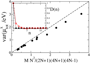
Figure 3: Main panel: numerically obtained variance of the sample-integrated spin-dependent potential $\mu_{\rm tot}^{(x)}$ in the RMT model (circles) vs. the theoretical prediction of Eq. (16) (dashed line) for $N_{L}=N_{R}=N\in[3,25]$ and $M\in[64,625]$. Deviations from the theory occur at smaller number of channels, for which fluctuations in the denominator of Eq. (9) can no longer be neglected. The behavior of $\mu_{\rm tot}^{(y)}$ and $\mu_{\rm tot}^{(z)}$ is the same as the one of $\mu_{\rm tot}^{(x)}$. Inset: spin-spin correlation function $D(n)=\langle S^{(\beta)}(i)S^{(\beta)}(i+na)\rangle$ for the RMT model (black circles) and the diffusive model (red squares) with $\ell=8a$, $\ell_{so}=12a$. In both cases, we find that the correlator does not depend on the spin orientation $\beta$.

Finally focusing on the RMT model, Fig. 3 confirms our main results, Eq. (14-15), by showing the scaling of the variance of the sample-integrated spin-dependent chemical potential in symmetric samples $N_{L}=N_{R}=N$ as a function of $N$ and the size $M$ of the random matrix Hamiltonian. Small deviations from our analytical predictions occur at small $N$ for which our procedure of replacing the denominator in Eq. (9) by its average squared when calculating ${\rm var}\,\mu_{P}^{(\beta)}$ is no longer justified. All these results numerically confirm our scattering theory of spin polarizations.

V Conclusions

We have demonstrated how introducing an external probe allows to relate local current-induced spin polarizations in a mesoscopic system to spin-resolved transmission coefficients. Focusing on ballistic systems, we used random matrix theory to compute the statistics of these polarizations. We predicted that a ballistic quantum dot with large contacts to external transport leads – but still large dwell time – typically carries a spin polarization that exceeds those previously investigated by a parametrically large factor [see Eqs. (3–5)]. Perhaps most importantly, we used this spin-probe model to calculate for the first time quantum correlations between local spin polarizations and spin currents, beyond the classical Fick law. We showed that the reported large spin polarizations correlate only weakly with spin currents, thus they cannot be easily converted into spin currents – and vice-versa. As disappointing as this result may be, it is consistent with the universality of spin current fluctuations Bar07 ; Naz07 ; Kri08 ; Ada09 .

The reported accumulations are coherent in nature, and one might wonder how they disappear as the system is coupled to external sources of noise. In this respect it is interesting to note that for a multichannel probe, Eq. (16) becomes, for $N,N_{P}\gg 1$,

$${\rm var}\,S_{\rm tot}^{(\beta)} \approx \frac{k_{\rm F}^{2}A}{144\pi N}\left(\frac{eV}{2\delta}\right)^{2}\frac{1}{(1+N_{P}/2N)^{3}}\,.$$ (25)

Enlarging the spin-probe damps the variance of the polarizations in a similar way as a dephasing probe damps conductance fluctuations But , with however a different parametric dependence on $N_{P}/N$. Note that the probe generating this damping is spin-conserving on time-average, as there is no spin current flowing through it.

Beside decoherence effects, there are a number of interesting open problems, related for instance to spatial fluctuations of spin polarizations and our assumption of a sharp decay of correlations at $k_{\rm F}^{-1}$. Finding out how the polarizations correlate to spin currents in diffusive systems, as well as in true ballistic systems treated beyond RMT is also of interest. Ways to extract the large typical polarizations we reported in the nonlinear transport regime or by optical means as in Ref. Kat04 should also be explored.

Appendix A

We demonstrate that the potentials ensuring zero current through a single-channel probe do not depend on the transparency of the contact between the probe and the system. According to Eq. (9), the chemical potentials in an external probe connected to a voltage-biased two-terminal cavity are given by the ratio of the difference and the sum of transmission coefficients between the transport leads and the probe. We show that the $\Gamma_{P}$-dependence of the coefficients $\mathcal{T}_{PI}^{(\alpha\beta)}$ factorizes when $N_{P}=1$ so that $\Gamma_{P}$ does not affect the chemical potential.

Our starting point is Eq. (20) for the scattering matrix, which we rewrite here,

$${\cal S}=1-2\pi iW^{\dagger}(E_{\rm F}-{\cal H}+i\pi WW^{\dagger})^{-1}W\,.$$ (26)

The matrix $WW^{\dagger}=VV^{\dagger}+PP^{\dagger}$ projects onto the system’s states coupled to the transport leads ($VV^{\dagger}$) and the probe ($PP^{\dagger}$). We can write a perturbative series in $PP^{\dagger}$ for the elements of the scattering matrix connecting the leads to the probe ($j_{I}$ is a channel index on the $I=L,R$ leads)

$${\cal S}_{P,j_{I}} = -2\pi i\sum_{x,x^{\prime}}P^{*}_{xP}V_{x^{\prime}j_{I}}\langle x|(E_{\rm F}-{\cal H}+i\pi WW^{\dagger})^{-1}|x^{\prime}\rangle$$ (27)

$$= -2\pi i\sum_{x,x^{\prime}}P^{*}_{xP}V_{x^{\prime}j_{I}}\left[\langle x|(E_{\rm F}-{\cal H}+i\pi VV^{\dagger})^{-1}|x^{\prime}\rangle\right.$$

$$\left.-i\pi\langle x|(E_{\rm F}-{\cal H}+i\pi VV^{\dagger})^{-1}PP^{\dagger}(E_{\rm F}-{\cal H}+i\pi VV^{\dagger})^{-1}|x^{\prime}\rangle+\ldots\right]\,.$$

The transparency of the contact between probe and system is contained exclusively in the matrix $P$. We are free to choose any orthogonal basis $\{|x\rangle\}$ for the system and pick one where the $M\times 1$ coupling matrix between probe and system is $P_{xP}=\omega_{P}\delta_{xP}$. One then has for the $M\times M$ matrix $\langle x|PP^{\dagger}|x^{\prime}\rangle=\langle P|PP^{\dagger}|P\rangle\delta_{xP}\delta_{x^{\prime}P}=|\omega_{P}|^{2}\delta_{xP}\delta_{x^{\prime}P}$, with $|\omega_{P}|^{2}=(M\delta/\pi^{2}\Gamma_{P})(2-\Gamma_{P}-2\sqrt{1-\Gamma_{P}})$ caveat3 . One gets

$${\cal S}_{Pj_{I}} = -2\pi i\omega_{p}^{*}\sum_{n=0}^{\infty}\left(-i\pi|\omega_{P}|^{2}\,\langle P|(E_{\rm F}-{\cal H}+i\pi VV^{\dagger})^{-1}|P\rangle\right)^{n}\times\sum_{x^{\prime}}V_{x^{\prime}j_{I}}\langle P|(E_{\rm F}-{\cal H}+i\pi VV^{\dagger})^{-1}|x^{\prime}\rangle$$ (28)

$$= f(\Gamma_{P})\times\sum_{x^{\prime}}V_{x^{\prime}j_{I}}\langle P|(E_{\rm F}-{\cal H}+i\pi VV^{\dagger})^{-1}|x^{\prime}\rangle\,.$$

One sees that, because the probe is single-channeled, the $\Gamma_{P}$-dependent part of ${\cal S}_{Pj_{I}}$ factorizes, and the same obviously holds for transmission coefficients ${\mathcal{T}}_{PI}^{(00)}=\sum_{j_{I}}|{\cal S}_{Pj_{I}}|^{2}$. This is not the case for a multichannel probe, in which case $|P\rangle$ is no longer unique. Thus, for $N_{P}=1$, the electrochemical potential in Eq. (10) do not depend on the strength of the tunnel barrier. The argument is straightforwardly extended to the spin-dependent chemical potentials in Eq. (9), because for a single-channel probe, the reflection coefficient ${\mathcal{T}}_{PP}^{(\alpha\beta)}$ is diagonal in spin-indices.

References

- (1) F.T. Vasko and N.A. Prima, Sov. Phys. Solid State 21, 994 (1979); L.S. Levitov, Y.V. Nazarov, and G.M. Eliashberg, Sov. Phys. JETP 61, 133 (1985); A.G. Aronov and Yu.B. Lyanda-Geller, JETP Lett. 50, 431 (1989).
- (2) V. M. Edelstein, Solid State Comm. 73, 233 (1990).
- (3) M.I. Dyakonov and V.I. Perel, Sov. Phys. JETP Lett. 13, 467 (1971).
- (4) For a review on the spin Hall effect, see: H.-A. Engel, E.I. Rashba, and B.I. Halperin, Theory of Spin Hall Effects in Semiconductors, Handbook of Magnetism and Advanced Magnetic Materials, Wiley and Sons (2007); arXiv:cond-mat/0603306.
- (5) Y.K. Kato, R.C. Myers, A. C. Gossard, and D. D. Awschalom, Science 306, 1910 (2004).
- (6) J. Wunderlich, B. Kästner, J. Sinova, and T. Jungwirth, Phys. Rev. Lett. 94, 047204 (2005).
- (7) S.O. Valenzuela and M. Tinkham, Nature 442, 176 (2006).
- (8) E. Saitoh, M. Ueda, H. Miyajima, and G. Tatara, Appl. Phys. Lett. 88, 182509 (2006); T. Kimura, Y. Otani, T. Sato, S. Takahashi, and S. Maekawa, Phys. Rev. Lett. 98, 156601 (2007); 98, 249901(E) (2007).
- (9) H. Zhao, E.J. Loren, H.M. van Driel, and A.L. Smirl, Phys. Rev. Lett. 96, 246601 (2006).
- (10) E.G. Mishchenko, A.V. Shytov, and B.I. Halperin, Phys. Rev. Lett. 93, 226602 (2004).
- (11) A.A. Burkov, A.S. Núez, and A.H. MacDonald, Phys. Rev. B 70 155308 (2004).
- (12) A.G. Mal’shukov, L.Y. Wang, C.S. Chu, and K.A. Chao, Phys. Rev. Lett. 95, 146601 (2005).
- (13) İ. Adagideli, M. Scheid, M. Wimmer, G.E.W. Bauer, and K. Richter, New J. Phys. 9, 382 (2007).
- (14) Y. Tserkovnyak, B.I. Halperin, A.A. Kovalev, and A. Brataas, Phys. Rev. B 76, 085319 (2007).
- (15) O. Chalaev and D. Loss, Phys. Rev. B 71, 245318 (2005).
- (16) J. H. Bardarson, İ. Adagideli, and Ph. Jacquod, Phys. Rev. Lett. 98, 196601 (2007).
- (17) Y. V. Nazarov, New J. Phys. 9, 352 (2007).
- (18) J. J. Krich and B. I. Halperin, Phys. Rev. B 78, 035338 (2008).
- (19) İ. Adagideli, J.H. Bardarson, and Ph. Jacquod, J. Phys.: Condens. Matter 21, 155503 (2009).
- (20) J.J. Krich, Phys. Rev. B 80, 245313 (2009).
- (21) B.K. Nikolić, L.P. Zârbo, and S. Souma, Phys. Rev. B 72, 075361 (2005).
- (22) W. Ren, Z. Qiao, J. Wang, Q. Sun, and H. Guo, Phys. Rev. Lett. 97, 066603 (2006).
- (23) M. Duckheim and D. Loss, Phys. Rev. Lett. 101, 226602 (2008).
- (24) P.W. Brouwer and C.W.J. Beenakker, J. Math. Phys. 37, 4904 (1996).
- (25) M.L. Mehta, Random Matrices, Academic Press, London (1990).
- (26) Because of Coulomb interactions, such a direct relation does not necessarily exist for the electrochemical potential on the dot, see e.g.: M. Büttiker, J. Phys.: Condens. Matter 5, 9361 (1993).
- (27) M. Büttiker, Phys. Rev. Lett. 57, 1761 (1986).
- (28) Y. Imry in Directions in Condensed Matter Physics, G. Grinstein and G. Mazenko eds., World Scientific, Singapore (1986).
- (29) For , gives the chemical potential difference between the two possible spin orientations along the corresponding spin axis, while gives the usual electrochemical potential. We refer to electrochemical and spin-dependent potentials collectively as “chemical potentials”. Note the plural. “Chemical potential” still retains its standard meaning.
- (30) F. Zhai and H.Q. Xu, Phys. Rev. Lett. 94, 246601 (2005); A.A. Kiselev and K.W. Kim, Phys. Rev. B 71, 153315 (2005).
- (31) M. Büttiker, Phys. Rev. B 40, 3409 (1989).
- (32) Correlated escape of pairs of classical trajectories and its influence on semiclassical transport was first discussed in: Ph. Jacquod and R.S. Whitney, Phys. Rev. B. 73 , 195115 (2006). The only nonvanishing semiclassical contributions to for have trajectories with correlated escape; Ph. Jacquod, unpublished (2008).
- (33) C. Mahaux and H.A. Weidenmüller, Shell-Model Approach to Nuclear Reactions, North-Holland, Amsterdam (1969).
- (34) M. Büttiker, Phys. Rev. B 33, 3020 (1986); H.U. Baranger and P.A. Mello, Waves in Random Media 9, 105 (1999).
- (35) The eigenvalue of is not uniquely determined by . Here we take the smallest of the two solutions, for which the expansion of Eq. (27) is guaranteed to converge.