Mixing-time and large-decoherence in continuous-time quantum walks on one-dimension regular networks

Abstract

In this paper, we study mixing and large decoherence in continuous-time quantum walks on one dimensional regular networks, which are constructed by connecting each node to its $2l$ nearest neighbors($l$ on either side). In our investigation, the nodes of network are represented by a set of identical tunnel-coupled quantum dots in which decoherence is induced by continuous monitoring of each quantum dot with nearby point contact detector. To formulate the decoherent CTQWs, we use Gurvitz model and then calculate probability distribution and the bounds of instantaneous and average mixing times. We show that the mixing times are linearly proportional to the decoherence rate. Moreover, adding links to cycle network, in appearance of large decoherence, decreases the mixing times.

1 Introduction

Quantum walks are the quantum counterpart of random walks, and were recently studied in the context of quantum information because of their prominent role in the design of quantum algorithms. Quantum walks were formulated in studies involving the dynamics of quantum diffusion [1], but the analysis of quantum walks for use in quantum algorithms was first done by Farhi and Gutmann [2]. Depending on the way the evolution operator is defined, quantum walks can be either discrete-time quantum walks(DTQWs) [3] or continuous-time quantum walks(CTQWs) [2]. In the CTQW, one can directly define the walk on the position space, whereas in the DTQW, it is necessary to introduce a quantum coin operation to define the direction in which the particle has to move. In recent years, many articles have studied the dynamics of the quantum walks on networks. For example, the DTQW has been studied in [4, 5, 6, 7] and the CTQW has been considered in [8, 9, 10, 11, 12, 13, 14, 15, 16, 17, 18]. One of the most important quantities have been defined for quantum walks analogous to random walks is mixing time. To introduce the mixing time, we refer to computer science. In many computational problems, the best solution can be found if we are able to sample from a well-chosen sampling distribution. This can be provided by mapping the uniform distribution into the desired one [19]. So, the behavior of many algorithms that use quantum(random) walks depends on the time it takes the walk to approach its uniform distribution, which is called the mixing time. In other words, the quantum(classical) algorithms are efficient if quantum(random) walks approach the uniform distribution fast. Since any practical implementation scheme of quantum walks must deal with decoherence, the natural question rises is: what parameters affect the mixing time of decoherent quantum walks. Several investigations on the decoherent quantum walks were given in [20, 21, 22, 23, 24, 25, 26]. Also, the mixing time of decoherent CTQWs on cycle graphs has been studied in [27]. In that work, the authors proved that the mixing time, for small rates of decoherence, improves linearly with decoherence, whereas for large rates of decoherence, deteriorates linearly towards the classical limit. But experimental implementation of quantum walks is done by physical systems including ground state atoms[28] and Rydberg atoms[29]. Some of the physical systems must deal with electromagnetism interactions extending to long distances. For example, the clouds of ultra cold Rydberg atoms assembled in a chain over which an exciton migrates, the trapping of the exciton occurs

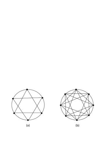
Figure 1: 1D regular networks with $N=6$, $l=2$ (a) and $N=8$ and $l=3$ (b).

at the ends of the chain. Therefore, we must take into account long-range interactions by adding links to cycle and then study the effects of these links on the CTQWs in the appearance of decoherence. In this article, we focus on one dimensional ($1D$) regular networks as generalized cycle networks having additional links and show that for large rates of decoherence, the bounds of instantaneous and average mixing times are proportional to decoherence parameter but decrease with increasing additional links (the problem for small decoherence is studied in [30]).
Our paper is structured as follows: We describe the structure of $1D$ regular network in Sec. 2. Sec. 3 provides a brief summary of the main concepts and of the formulae concerning CTQWs and give the exact solutions to the transition probabilities on $1D$ regular network. Sec. 4 presents the decoherent CTQWs on $1D$ regular network. We assume that the decoherence rate is large and calculate the probability distribution in Sec. 5. In Sec. 6, we obtain the lower and upper bounds of instantaneous and average mixing times. Conclusions and discussions are given in the last part, Sec. 7.

2 Structure of $1D$ regular network

$1D$ networks are composed of a cycle graph of $N$ nodes in which every node is connected to its $2l$ nearest neighbors($l$ on either side) [31], where $N$ is the network size and $l$ is the interaction parameter, i.e. all the two nodes whose distance is smaller than or equal to $l$ are connected by additional bonds. Figs. 1(a) , (b) show sketches of $1D$ regular networks with $N=6,l=2$ and $N=8,l=3$, respectively. These networks provide a good model to study various coupled dynamical systems, including biological oscillators [32], Josephson junction arrays [33], synchronization [34], small-world networks [35] and many other self-organizing systems.

3 CTQWs on $1D$ regular network

Every network can be considered as a graph made up of nodes and algebraically described by the so-called adjacency matrix $A=(A_{ij})$, which is a discrete version of the Laplace operator. The non-diagonal elements $A_{ij}$ equal 1 if nodes $i$ and $j$ are connected by a bond and 0 otherwise. The connectivity of node $i$ can be calculated as a sum of matrix elements $z_{i}=\sum_{j}A_{ij}$. The Laplacian operator is then defined as $L=Z-A$, where $Z$ is the diagonal matrix given by $Z_{ik}=z_{i}\delta_{ik}$. It is worth underlining that, being symmetric and non-negative definite, $L$ can generate both probability conserving Markov process and unitary process. Thus, the Laplacian operator can work both as a classical transfer operator and as a tight-binding Hamiltonian of quantum transport process [36, 37, 38].
The continuous-time random walks(CTRWs) are described by the following Master equation [39]:

$$\frac{d}{dt}p_{k,j}(t)=\sum_{l=1}^{N}T_{kl}p_{l,j}(t),$$ (1)

being $p_{k,j}(t)$ the conditional probability that the walker is on node $k$ at time $t$ when it started from node $j$. If the walk is symmetric with a site-independent transmission rate $\gamma$, then the transfer matrix $T$ is simply related to the Laplacian operator through $T=-\gamma L$(in the following we set $\gamma=1$).
The quantum-mechanical extension of the CTRW is called continuous-time quantum walk(CTQW). The CTQWs are obtained by identifying the Hamiltonian of the system with the classical transfer matrix, $H=-T$ [2, 37, 40]. The states $|j\rangle$, representing the walker localized at the node $j$, span the whole accessible Hilbert space and also provide an orthonormal basis set. In these basis the Schrödinger equation is

$$i\frac{d}{dt}|k\rangle=H|k\rangle,$$ (2)

where we set $m=1$ and $\hbar=1$. The time evolution of state $|j\rangle$ starting at time 0 is given by $|j,t\rangle=U(t)|j\rangle$, where $U(t)=\exp[-iHt]$ is the quantum-mechanical time evolution operator. Therefore, the behaviour of the walker can be described by the transition amplitude $\alpha_{k,j}(t)$ from state $|j\rangle$ to state $|k\rangle$, which is

$$\alpha_{k,j}(t)=\langle k|e^{-iHt}|j\rangle.$$ (3)

From Eq. (2), the $\alpha_{k,j}(t)$ obeys the following Schrödinger equation:

$$\frac{d}{dt}\alpha_{k,j}(t)=-i\sum_{l=1}^{N}H_{kl}\alpha_{l,j}(t).$$ (4)

Note that the squared magnitude of transition amplitude provides the quantum-mechanical transition probability $\pi_{k,j}(t)=|\alpha_{k,j}(t)|^{2}$.
To get the exact solution of Eqs. (1) and (4), all the eigenvalues and eigenvectors of the transfer operator and Hamiltonian are required. We denote the nth eigenvalue and eigenvector of $H$ by $E_{n}$ and $|q_{n}\rangle$, respectively. Now, by using the formal solution, the classical probability is given by

$$p_{k,j}(t)={\langle k|e^{Tt}|j\rangle=\langle k|e^{-Ht}|j\rangle}=\sum_{n=1}^{N}e^{-tE_{n}}\langle k|q_{n}\rangle\langle q_{n}|j\rangle,$$ (5)

and the quantum-mechanical transition probability can write as

$$\pi_{k,j}(t)=\sum_{n,l=1}^{N}e^{-it(E_{n}-E_{l})}\langle k|q_{n}\rangle\langle q_{n}|j\rangle\langle q_{l}|k\rangle\langle j|q_{l}\rangle,$$ (6)

In the following, we focus on $1D$ regular networks and study CTQWs on them. The Hamiltonian of the system is given by [30]

$$H_{ij}=\left\{\begin{array}[]{ll}-2l,&\hbox{if $i=j$;}\\ 1,&\hbox{if $i=j\pm m,m\in[1,l]$;}\\ 0,&\hbox{Otherwise.}\end{array}\right.$$ (10)

This Hamiltonian acting on the state $|j\rangle$ can be written as

$$H|j\rangle=-(2l+1)|j\rangle+\sum_{m=-l}^{l}|j+m\rangle.$$ (11)

which is the discrete version of the Hamiltonian for a free particle moving on a lattice. It is well known in solid state physics that the solutions of the Schrödinger equation for a particle moving freely in a regular potential are Bloch functions [41, 42]. We denote the Bloch states by $|\Phi_{n}\rangle$ and then the time independent Schrodinger equation can be written as

$$H|\Phi_{n}\rangle=E_{n}|\Phi_{n}\rangle.$$ (12)

The Bloch state $|\Phi_{n}\rangle$ can be expressed as a linear combination of the states $|j\rangle$ localized at nodes $j$,

$$|\Phi_{n}\rangle=\frac{1}{\sqrt{N}}\sum_{j=0}^{N-1}e^{-i\theta_{n}j}|j\rangle.$$ (13)

Because of periodic boundary conditions, we have $\Phi_{n}(N)=\Phi_{n}(0)$, where $\Phi_{n}(x)=\langle x|\Phi_{n}\rangle$. This restricts the $\theta_{n}$-values to $\theta_{n}=\frac{2\pi n}{N}$, where $n=0,1,\ldots,N-1$. We set Eq. (8) and (10) into (9) and obtain the eigenvalues of system as [30]

$$E_{n}=-2l+2\sum_{j=1}^{l}\cos(j\theta_{n}).$$ (14)

Thus Eq. (5) and (6) can be written as

$$p_{k,j}(t)=\frac{1}{N}\sum_{n}e^{-tE_{n}}e^{-i(k-j)\frac{2n\pi}{N}},$$ (15)

$$\pi_{k,j}(t)=\frac{1}{N^{2}}\sum_{n,l}e^{-it(E_{n}-E_{l})}e^{-i(k-j)(n-l)\frac{2\pi}{N}}.$$ (16)

4 The Decoherent CTQWs on $1D$ regular network

In this section, we take into account the effects of decoherence in quantum walks on $1D$ regular network. For this aim, we consider the model of network in which decoherence is induced by continuous monitoring of each network node with nearby point contact(PC) detector. In this model, our assumptions are as follows: each node is represented by a quantum dot which is continuously monitored by an individual point contact(PC), the walks are performed by an electron initially placed in one of the quantum dots, identical PCs are placed far enough from QDs so that the tunneling between them is negligible, Coulomb interaction between electrons in QD and PC is taken into account and all electrons are spin-less fermions [43]. With help of gate-engineering techniques in semiconductor heterostructures, the quantum dots cycle (the 1D regular graphs are a kind of cycle graphs) with attached point contacts can be constructed[44]. Such techniques allow electronically to make of quantum dots and point contact by placing metal gates on the structure with a two-dimensional electron gas. By changing the potential on gates one can assign area of two-dimensional electron gas

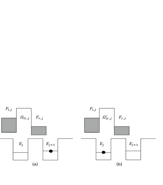
Figure 2: Fig. 2(a) shows point contact detector $j$ monitoring the electron in dot $j+1$ and Fig. 2(b) shows point contact detector $j$ when electron is placed in dot $j$. Source and drain reservoirs are kept at zero temperature with chemical potentials $F_{l,j}$ and $F_{r,j}$, respectively. $E_{j}$ is the on-site node energy. $\Omega_{lr,j}$ and $\Omega^{\prime}_{lr,j}$ are transmission probability of the detector for empty dot and for the occupied dot.

which creates the necessary confinement profile [43]. In Ref. [45], the simplest example of such structure which contains two quantum dots was experimentally investigated. Such a set up is shown schematically in Fig. 2, where detector $j$ is represented by a barrier, connected with two reservoirs at the potentials $F_{l,j}$ and $F_{r,j}$. The transmission probability of the barrier varies from $\Omega_{lr,j}$ to $\Omega^{\prime}_{lr,j}$, depending on whether or not the quantum dot is occupied by an electron. In the following, we want to write the Hamiltonian for the entire system. We consider simple continuous-time quantum walks are defined over an undirected graph with $N$ nodes in which each node corresponds by an integer $j\in[0,N-1]$ and a quantum state $|j\rangle$. These walks can be well described by the following Hamiltonian [19, 46]:

$$\begin{array}[]{cc}H_{s}=&\displaystyle\sum_{ij}\Delta_{ij}(t)(\hat{c}^{{\dagger}}_{i}\hat{c}_{j}+\hat{c}_{i}\hat{c}^{{\dagger}}_{j})-\displaystyle\sum_{j}E_{j}(t)\hat{c}^{{\dagger}}_{j}\hat{c}_{j},\\ &\\ =&\displaystyle\sum_{ij}\Delta_{ij}(t)(|i\rangle\langle j|+|j\rangle\langle i|)+\displaystyle\sum_{j}E_{j}(t)|j\rangle\langle j|.\end{array}$$ (20)

where $\hat{c}^{{\dagger}}_{i}(\hat{c}_{j})$ are creation (annihilation) operators such that $\hat{c}^{{\dagger}}_{i}\hat{c}_{j}$ acting on a state at node $j$ brings it to node $i$. So, state $|j\rangle$ denoting the state of particle at node $j$ can be obtained by acting $c^{{\dagger}}_{j}$ on the ground state $|0\rangle$. The two terms correspond to a hopping term with amplitudes $\triangle_{ij}(t)$ between nodes, and on-site node energies $E_{j}(t)$, both of which can depend on time. For the sake of simplicity, we drop all the on-site energies(i.e. $E_{j}=0,\forall j$) and assume that hopping amplitudes($\triangle_{ij}(t)$) between connected sites to be constant. Also, we renormalize the time, so that it becomes dimensionless [43]. Thus, Eq. (14) for $1D$ regular networks is written as

$$H_{s}=\frac{1}{4}\sum_{j=0}^{N-1}\sum_{z=1}^{l}(\hat{c}^{\dagger}_{j+z}\hat{c}_{j}+\hat{c}^{{\dagger}}_{j}c_{j+z}).$$ (21)

Now, we study the electron transport process in point contact $j$. The point contact is considered as a barrier, separated two reservoirs(the source and drain). All the levels in the source and drain are initially filled up to the Fermi energies, which is called the vacuum state $|0\rangle$. Thus, the Hamiltonian of $j$-th point contact can be written as

$$H_{pc,j}=\sum_{l}E_{l,j}\hat{a}^{\dagger}_{l,j}\hat{a}_{l,j}+\sum_{r}E_{r,j}\hat{a}^{\dagger}_{r,j}\hat{a}_{r,j}+\sum_{l,r}\Omega_{lr,j}(\hat{a}^{\dagger}_{l,j}\hat{a}_{r,j}+\hat{a}^{\dagger}_{r,j}\hat{a}_{l,j}),$$ (22)

where $\hat{a}^{\dagger}_{l,j}(\hat{a}_{l,j})$ and $\hat{a}^{\dagger}_{r,j}(\hat{a}_{r,j})$ are the creation(annihilation) operators in the left and right reservoirs respectively, and $\Omega_{lr,j}$ is the hopping amplitude between the states $E_{l,j}$ and $E_{r,j}$ in the right and left reservoirs.
The interaction between the detector and the measured system is described by $H_{int}$. The presence of an electron in the left dot results in an effective increase of the point contact barrier($\acute{\Omega_{lr,j}}=\Omega_{lr,j}+\delta\Omega_{lr,j}$). Therefore, the interaction Hamiltonian can be written as

$$H_{int}=\sum_{l,r}\delta\Omega_{lr,j}\hat{c}_{j}^{\dagger}\hat{c}_{j}(\hat{a}_{l,j}^{\dagger}\hat{a}_{r,j}+\hat{a}^{\dagger}_{r,j}\hat{a}_{l,j}).$$ (23)

For simplicity, we assume that the hoping amplitudes are weakly dependent on states $E_{l,j}$ and $E_{r,j}$, so that $\Omega_{lr,j}=\bar{\Omega}$, $\delta\Omega_{lr,j}=\delta\bar{\Omega}$ and $F_{l,j}(F_{r,j})=\bar{F_{l}}(\bar{F_{r}})$. The decoherence rate $\Gamma$ can be written as $\Gamma=\delta\bar{\Omega}^{2}(\bar{F}_{r}-\bar{F}_{l})^{2}f_{S}f_{D}$ where $f_{S}$ and $f_{D}$ are density of states in source and reservoirs, respectively [43]. Gurvitz in [47] showed that the appearance of decoherence leads to the collapse of the density matrix into the statistical mixture in the course of the measurement processes, thus the evolution of the reduced density matrix traced over all states of source and drain electrons is given by Bloch-type rate equations. The time dependent non-unitary evolution of reduced density matrix $\rho(t)=|\Phi(t)\rangle\langle\Phi(t)|$ in the Gurvitz model is given by [30]

$$\begin{array}[]{cc}\frac{d}{dt}\rho_{j,k}(t)=&-\frac{i}{4}[\displaystyle\sum_{m=-l}^{l}(\rho_{j+m,k}-\rho_{j,k+m})]-\Gamma(1-\delta_{j,k})\rho_{j,k}\\ &\\ =&-\frac{i}{4}[\displaystyle\sum_{m=1}^{l}(\rho_{j+m,k}-\rho_{j,k+m}+\rho_{j-m,k}-\rho_{j,k-m})]-\Gamma(1-\delta_{j,k})\rho_{j,k}.\end{array}$$ (27)

5 Large Decoherence

In [30], authors studied the effect of small decoherence($\Gamma N\ll 1$) in CTQWs on $1D$ regular networks. They showed that the instantaneous mixing time upper bound and the average time mixing lower bound are independent of parameter $l(l\geq 2)$, but are proportional to the inverse of decoherence rate. Here, we want to study CTQWs on these networks in appearance of the large rates of decoherence. For this purpose, we use Gurvitz model and focus on the elements of matrix $\rho(t)$. Based on the initial conditions, the non-zero elements appear only along the major diagonal. Firstly, we rewrite Eq. (18) for the elements of major diagonal and also minor diagonals whose distances of the major diagonal are lesser than $l$. By dropping terms that are smaller than $1/\Gamma$, we have

$$\left\{\begin{array}[]{ll}\rho^{\prime}_{j,j}(t)=-\frac{i}{4}[\displaystyle\sum_{m=1}^{l}(\rho_{j+m,j}-\rho_{j,j+m}+\rho_{j-m,j}-\rho_{j,j-m})],\\ &\\ \rho^{\prime}_{j,j+1}(t)=-\frac{i}{4}[\rho_{j+1,j+1}-\rho_{j,j}]-\Gamma\rho_{j,j+1},\\ &\\ \rho^{\prime}_{j,j+2}(t)=-\frac{i}{4}[\rho_{j+2,j+2}-\rho_{j,j}]-\Gamma\rho_{j,j+2},\\ \vdots\\ \rho^{\prime}_{j,j+l}(t)=-\frac{i}{4}[\rho_{j+l,j+l}-\rho_{j,j}]-\Gamma\rho_{j,j+l},\end{array}\right.$$ (35)

For the simplicity sake, we use the following definitions

$$\begin{array}[]{cc}a_{j}=\rho_{j,j}\\ d_{j}=\rho_{j,j+1}-\rho_{j+1,j},\\ f_{j}=\rho_{j,j+2}-\rho_{j+2,j},\\ \vdots&\\ q_{j}=\rho_{j,j+l}-\rho_{j+l,j}.&\end{array}$$ (41)

Then the above difference equation system can be written as

$$\left\{\begin{array}[]{ll}a^{\prime}_{j}=-\frac{i}{4}[-d_{j}+d_{j-1}-f_{j}+f_{j-2}+\cdots-q_{j}+q_{j-l}],\\ \\ d^{\prime}_{j}=-\frac{i}{2}[a_{j+1}-a_{j}]-\Gamma d_{j},\\ &\\ f^{\prime}_{j}=-\frac{i}{2}[a_{j+2}-a_{j}]-\Gamma f_{j},\\ \vdots\\ q^{\prime}_{j}=-\frac{i}{2}[a_{j+l}-a_{j}]-\Gamma q_{j},\\ \end{array}\right.$$ (49)

Differentiation of the above equation gives

$$\left\{\begin{array}[]{ll}a^{\prime\prime}_{j}=-\frac{i}{4}[-d^{\prime}_{j}+d^{\prime}_{j-1}-f^{\prime}_{j}+f^{\prime}_{j-2}+\cdots-q^{\prime}_{j}+q^{\prime}_{j-l}],\\ \\ d^{\prime\prime}_{j}=-\frac{i}{2}[a^{\prime}_{j+1}-a^{\prime}_{j}]-\Gamma d^{\prime}_{j},\\ &\\ f^{\prime\prime}_{j}=-\frac{i}{2}[a^{\prime}_{j+2}-a^{\prime}_{j}]-\Gamma f^{\prime}_{j},\\ \vdots\\ q^{\prime\prime}_{j}=-\frac{i}{2}[a^{\prime}_{j+l}-a^{\prime}_{j}]-\Gamma q^{\prime}_{j},\\ \end{array}\right.$$ (57)

We can guess the following solutions for the above equations

$$\begin{array}[]{ccc}a_{j}=\displaystyle\sum_{k=0}^{N-1}A_{k}e^{\frac{2\pi ijk}{N}}e^{-\gamma_{k}t},&&d_{j}=\displaystyle\sum_{k=0}^{N-1}D_{k}e^{\frac{2\pi ijk}{N}}e^{-\gamma_{k}t},\\ &&\\ f_{j}=\displaystyle\sum_{k=0}^{N-1}F_{k}e^{\frac{2\pi ijk}{N}}e^{-\gamma_{k}t},&\cdots,&q_{j}=\displaystyle\sum_{k=0}^{N-1}Q_{k}e^{\frac{2\pi ijk}{N}}e^{-\gamma_{k}t},\end{array}$$ (61)

in which $\gamma_{k}$, $A_{k}$, $D_{k}$,$\cdots$ and $Q_{k}$ are the unknown quantities. Then, we set these solutions into Eqs. (22) and get

$$\left\{\begin{array}[]{ll}\gamma_{k}A_{k}+\frac{i}{4}[D_{k}(1-e^{\frac{-2\pi ik}{N}})+F_{k}(1-e^{\frac{-4\pi ik}{N}})+\cdots+Q_{k}(1-e^{\frac{-2\pi ikl}{N}})]=0\\ &\\ A_{k}[\frac{i}{2}(-e^{\frac{2\pi ik}{N}}+1)]+D_{k}(\gamma_{k}-\Gamma)=0,\\ &\\ A_{k}[\frac{i}{2}(-e^{\frac{4\pi ik}{N}}+1)]+F_{k}(\gamma_{k}-\Gamma)=0,\\ \vdots\\ A_{k}[\frac{i}{2}(-e^{\frac{2l\pi ik}{N}}+1)]+Q_{k}(\gamma_{k}-\Gamma)=0,\end{array}\right.$$ (69)

It is evident that there are nontrivial solutions for the set of equations if the determinant of the coefficients matrix is zero.

$$(\gamma_{k}-\Gamma)^{(l-1)}[\gamma_{k}(\gamma_{k}-\Gamma)+\frac{1}{2}(\sin^{2}(\frac{\pi k}{N})+\sin^{2}(\frac{2\pi k}{N})+\cdots+\sin^{2}(\frac{l\pi k}{N}))]=0$$ (70)

Therefore, four values for $\gamma_{k}$ are obtained as

$$\gamma_{k}=\left\{\begin{array}[]{ll}\gamma_{k,0}=0,\\ \gamma_{k,1}=\Gamma,\\ \gamma_{k,2}=\Gamma-\displaystyle\frac{1}{2\Gamma}\displaystyle\sum_{m=1}^{l}\sin^{2}(\frac{\pi km}{N}),\\ \gamma_{k,3}=\displaystyle\frac{1}{2\Gamma}\displaystyle\sum_{m=1}^{l}\sin^{2}(\frac{\pi km}{N}),\end{array}\right.$$ (75)

The general solutions of Eqs. (22) are

$$\left\{\begin{array}[]{ll}a_{j}=\frac{1}{N}\displaystyle\sum_{k=0}^{N-1}\{A_{k,0}e^{-\gamma_{k,0}t}+A_{k,1}e^{-\gamma_{k,1}t}+A_{k,2}e^{-\gamma_{k,2}t}+A_{k,3}e^{-\gamma_{k,3}t}\}\omega^{jk},\\ \\ d_{j}=\frac{1}{N}\displaystyle\sum_{k=0}^{N-1}\{D_{k,0}e^{-\gamma_{k,0}t}+D_{k,1}e^{-\gamma_{k,1}t}+D_{k,2}e^{-\gamma_{k,2}t}+D_{k,3}e^{-\gamma_{k,3}t}\}\omega^{jk},\\ \\ f_{j}=\frac{1}{N}\displaystyle\sum_{k=0}^{N-1}\{F_{k,0}e^{-\gamma_{k,0}t}+F_{k,1}e^{-\gamma_{k,1}t}+F_{k,2}e^{-\gamma_{k,2}t}+F_{k,3}e^{-\gamma_{k,3}t}\}\omega^{jk},\\ \vdots\\ q_{j}=\frac{1}{N}\displaystyle\sum_{k=0}^{N-1}\{Q_{k,0}e^{-\gamma_{k,0}t}+F_{k,1}e^{-\gamma_{k,1}t}+F_{k,2}e^{-\gamma_{k,2}t}+F_{k,3}e^{-\gamma_{k,3}t}\}\omega^{jk},\end{array}\right.$$ (83)

where $\omega=e^{\frac{2\pi i}{N}}$. By the initial condition $a_{j}(0)=\delta_{j,0}$ and $d_{j},f_{j},...,q_{j}(0)=0$, for $j=0,\cdots,N-1$, and replacing the constant coefficients into the others, we get

$$\left\{\begin{array}[]{ccc}A_{k,1}\simeq 0,&A_{k,2}\simeq\frac{-1}{2\Gamma^{2}}\displaystyle\sum_{m=1}^{l}\sin^{2}(\frac{\pi km}{N}),&A_{k,3}=1,\\ \\ D_{k,1}\simeq 0,&D_{k,2}\simeq\frac{i}{\Gamma}\sin(\frac{\pi k}{N})\exp(\frac{i\pi k}{N}),&D_{k,3}\simeq\frac{-i}{\Gamma}\sin(\frac{\pi k}{N})\exp(\frac{i\pi k}{N}),\\ \\ F_{k,1}\simeq 0,&F_{k,2}\simeq\frac{i}{\Gamma}\sin(\frac{2\pi k}{N})\exp(\frac{2i\pi k}{N}),&F_{k,3}\simeq\frac{-i}{\Gamma}\sin(\frac{2\pi k}{N})\exp(\frac{2i\pi k}{N}),\\ \vdots\\ Q_{k,1}\simeq 0,&Q_{k,2}\simeq\frac{i}{\Gamma}\sin(\frac{l\pi k}{N})\exp(\frac{li\pi k}{N}),&Q_{k,3}\simeq\frac{-i}{\Gamma}\sin(\frac{l\pi k}{N})\exp(\frac{li\pi k}{N}).\end{array}\right.$$ (91)

Note that the probability distribution $P(t)$ of the quantum walk is specified by the diagonal elements of $\rho(t)$, that is $P_{j}(t)=a_{j}(t)$. For our problem, this distribution reduces to

$$a_{j}(t)=\frac{1}{N}\displaystyle\sum_{k=0}^{N-1}\exp[-\frac{t\sum_{m=1}^{l}\sin^{2}(\frac{\pi km}{N})}{2\Gamma}]\omega^{jk}$$ (92)

Since CTQWs are symmetric under time-inversion, the above distribution does not converge to any constant value.

6 Mixing time

In this section, we discuss the rate of convergence to the above probability distribution which can be expressed in terms of mixing time. There are two distinct notations of mixing time in the literature: the instantaneous mixing time and the average mixing time. In the following, we give the definition of the two notations of mixing time in the continuous-time quantum walks on graphs and calculate them for our network.

(a) Instantaneous mixing time
The instantaneous mixing time focuses on particular times at which the probability distribution is sufficiently close to the uniform distribution [19], i.e. $t_{ins}$ is the instantaneous mixing time if

$$t_{ins}=min\{t:\sum_{j=0}^{N-1}\|P_{j}(t)-\frac{1}{N}\|\leq\epsilon\},$$ (93)

where $||p-q||=\sum_{i}|p_{i}-q_{i}|$ denotes the total variation distance between the distributions $p$ and $q$.
Adding a summation over $j$ to Eq. (29) gives us the total variation distance required to get the mixing time:

$$\begin{array}[]{cc}\displaystyle\sum_{j=0}^{N-1}|a_{j}(t)-\frac{1}{N}|&=\displaystyle\sum_{j=0}^{N-1}|\frac{1}{N}\sum_{k=0}^{N-1}\exp[\frac{-t}{2\Gamma}\displaystyle\sum_{m=1}^{l}\sin^{2}(\frac{\pi km}{N})]\omega^{jk}-\frac{1}{N}|\\ &\\ &=\displaystyle\sum_{j=0}^{N-1}|\frac{1}{N}\displaystyle\sum_{k=1}^{N-1}\exp[\frac{-t}{2\Gamma}\displaystyle\sum_{m=1}^{l}\sin^{2}(\frac{\pi km}{N})]\cos(\frac{2\pi jk}{N})|\end{array}$$ (97)

Lower bound
To find the lower bound, we use the term $j=0$ only

$$\begin{array}[]{cc}\displaystyle\sum_{j=0}^{N-1}|a_{j}(t)-\frac{1}{N}|&>|a_{0}(t)-\displaystyle\frac{1}{N}|=\displaystyle\frac{1}{N}|\displaystyle\sum_{k=1}^{N-1}\exp[\frac{-t}{2\Gamma}\displaystyle\sum_{m=1}^{l}\sin^{2}(\frac{\pi km}{N})]|\\ \end{array}$$ (99)

then consider the terms $k=1,N-1$

$$\begin{array}[]{cc}\displaystyle\sum_{j=0}^{N-1}|a_{j}(t)-\frac{1}{N}|&>\displaystyle\frac{2}{N}e^{-\displaystyle\frac{t}{2\Gamma}\displaystyle\sum_{m=1}^{l}\sin^{2}(\frac{\pi m}{N})}.\end{array}$$ (101)

It reaches $\epsilon$ at time $t_{ins,lower}$ when

$$\frac{2}{N}e^{-\displaystyle\frac{t_{ins,lower}}{2\Gamma}\displaystyle\sum_{m=1}^{l}\sin^{2}(\displaystyle\frac{\pi m}{N})}=\epsilon.$$ (102)

Finally, the instantaneous mixing time lower bound is obtained as

$$t_{ins,lower}=\frac{2\Gamma}{\displaystyle\sum_{m=1}^{l}\sin^{2}(\frac{\pi m}{N})}\ln(\frac{2}{N\epsilon}).$$ (103)

Note that for $l=1$ and large $N\gg 1$, we have

$$t_{ins,lower}=\frac{2\Gamma}{\sin^{2}(\frac{\pi}{N})}\ln(\frac{2}{N\epsilon})\simeq\frac{2\Gamma N^{2}}{\pi^{2}}\ln(\frac{2}{N\epsilon})$$ (104)

which is in agreement with [27]’s result for cycle.

Upper bound
An upper bound on the instantaneous mixing time can also be derived. To do this, first we find an upper bound for Eq. (31) by using the relation $|\cos(\frac{2\pi jk}{N})|<1$ for $k,j\neq 0,N$.

$$\begin{array}[]{cc}\displaystyle\sum_{j=0}^{N-1}|a_{j}(t)-\frac{1}{N}|<\displaystyle\frac{1}{N}\displaystyle\sum_{j=0}^{N-1}\displaystyle\sum_{k=1}^{N-1}\exp[\frac{-t}{2\Gamma}\displaystyle\sum_{m=1}^{l}\sin^{2}(\frac{\pi km}{N})]\\ &\\ <\displaystyle\frac{2}{N}\displaystyle\sum_{j=0}^{N-1}\displaystyle\sum_{k=1}^{[N/2]}\exp[\frac{-t}{2\Gamma}\displaystyle\sum_{m=1}^{l}\sin^{2}(\frac{\pi km}{N})]\\ \end{array}$$ (108)

Since $\sin(x)>\frac{2x}{\pi}$ for $0<x<\frac{\pi}{2}$ [48] , we have

$$\begin{array}[]{cc}\displaystyle\sum_{j=0}^{N-1}|a_{j}(t)-\frac{1}{N}|<\displaystyle\frac{2}{N}\displaystyle\sum_{j=0}^{N-1}\displaystyle\sum_{k=1}^{[N/2]}\exp[\frac{-t}{\Gamma}\displaystyle\sum_{m=1}^{l}\frac{2k^{2}}{N^{2}m^{2}}]\\ \end{array}$$ (110)

and by using $k^{2}\geq k$ when $k\geq 1$, we get

$$\begin{array}[]{cc}\displaystyle\sum_{j=0}^{N-1}|a_{j}(t)-\frac{1}{N}|<&\displaystyle\frac{2}{N}\displaystyle\sum_{j=0}^{N-1}\displaystyle\sum_{k=1}^{\infty}\exp[\frac{-t}{\Gamma}\displaystyle\sum_{m=1}^{l}\frac{2k}{N^{2}m^{2}}]\end{array}$$ (112)

After some algebra, we obtain

$$\sum_{j=0}^{N-1}|a_{j}(t)-\frac{1}{N}|<\frac{2}{\exp[{\displaystyle\frac{t}{\Gamma}\displaystyle\sum_{m=1}^{l}\frac{2}{N^{2}m^{2}}}]-1}.$$ (113)

According to the instantaneous mixing time definition(Eq.(30)):

$$\frac{2}{\exp[{\displaystyle\frac{t_{ins,upper}}{\Gamma}\displaystyle\sum_{m=1}^{l}\frac{2}{N^{2}m^{2}}}]-1}=\epsilon.$$ (114)

Therefore, the upper bound of instantaneous mixing time is

$$t_{ins,upper}=\frac{\Gamma N^{2}}{2\displaystyle\sum_{m=1}^{l}m^{-2}}\ln(\frac{2+\epsilon}{\epsilon}).$$ (115)

Moreover, for $l=1$(cycle), we obtain

$$t_{ins,upper}=\frac{\Gamma N^{2}}{2}\ln(\frac{2+\epsilon}{\epsilon})$$ (116)

which is the same result mentioned in [27].

(b) Average mixing time
The average mixing time which is based on the time-averaged probability distribution

$$\bar{P}(j,T)=\frac{1}{T}\int_{0}^{T}P(j,t)dt,$$ (117)

is the time it takes the average distribution to be $\epsilon$-close to the uniformly distributed [49], i.e. $t_{ave}$ is the average mixing time if

$$t_{ave}=min\{t:\|\bar{P}(j,T)-\frac{1}{N}\|\leq\epsilon\}.$$ (118)

where $||.||$ is the total variation distance mentioned in the instantaneous mixing time. To get the bounds of average mixing time, first we calculate $\bar{P}(j,T)$ by Eq. (29)

$$\begin{array}[]{cc}\bar{P}(j,T)&=\displaystyle\frac{1}{T}\displaystyle\int_{0}^{T}\displaystyle\frac{1}{N}\displaystyle\sum_{k=0}^{N-1}\exp[-\displaystyle\frac{t}{2\Gamma}\displaystyle\sum_{m=1}^{l}\sin^{2}(\frac{\pi km}{N})]\omega^{jk}dt\\ &\\ &=\displaystyle\frac{2\Gamma}{TN}\displaystyle\sum_{k=0}^{N-1}\displaystyle\frac{1-\exp[-\displaystyle\frac{T}{2\Gamma}\displaystyle\sum_{m=1}^{l}\sin^{2}(\frac{\pi km}{N})]\omega^{jk}}{\displaystyle\sum_{m=1}^{l}\sin^{2}(\frac{\pi km}{N})}\end{array}$$ (122)

The total variation distance between the uniform distribution and the time-average distribution of the decoherent quantum walk is given by

$$\begin{array}[]{cc}\displaystyle\sum_{j=0}^{N-1}|\bar{P}(j,T)-\frac{1}{N}|&=\displaystyle\sum_{j=0}^{N-1}|\displaystyle\frac{2\Gamma}{TN}\displaystyle\sum_{k=0}^{N-1}\displaystyle\frac{1-\exp[-\displaystyle\frac{T}{2\Gamma}\displaystyle\sum_{m=1}^{l}\sin^{2}(\displaystyle\frac{\pi km}{N})]\omega^{jk}}{\displaystyle\sum_{m=1}^{l}\sin^{2}(\displaystyle\frac{\pi km}{N})}-\displaystyle\frac{1}{N}|\\ &\\ &=\displaystyle\sum_{j=0}^{N-1}|\displaystyle\frac{2\Gamma}{TN}\displaystyle\sum_{k=1}^{N-1}\displaystyle\frac{1-\exp[-\displaystyle\frac{T}{2\Gamma}\displaystyle\sum_{m=1}^{l}\sin^{2}(\displaystyle\frac{\pi km}{N})]\omega^{jk}}{\displaystyle\sum_{m=1}^{l}\sin^{2}(\displaystyle\frac{\pi km}{N})}|\\ \end{array}$$ (126)

Lower bound
Now, we can find a lower bound for the average mixing time. As with the lower bound of instantaneous mixing time, we use the terms $j=0,k=1,N-1$.

$$\begin{array}[]{cc}\displaystyle\sum_{j=0}^{N-1}|\bar{P}(j,T)-\frac{1}{N}|&>\displaystyle\frac{4\Gamma}{TN}\displaystyle\frac{1-\exp[-\displaystyle\frac{T}{2\Gamma}\displaystyle\sum_{m=1}^{l}\sin^{2}(\displaystyle\frac{\pi m}{N})]}{\displaystyle\sum_{m=1}^{l}\sin^{2}(\displaystyle\frac{\pi m}{N})}\end{array}$$ (128)

Assume $T/\Gamma\gg 1$ (which is consistent with our other assumptions, $N\gg 1$ and $\Gamma N\gg 1$, it requires $T\gg N$) which results in

$$\displaystyle\sum_{j=0}^{N-1}|\bar{P}(j,T)-\frac{1}{N}|>\displaystyle\frac{4\Gamma}{TN\displaystyle\sum_{m=1}^{l}\sin^{2}(\displaystyle\frac{\pi m}{N})}$$ (129)

Therefore, the lower bound of average mixing time is

$$t_{ave,lower}=\frac{4\Gamma}{\epsilon N\sum_{m=1}^{l}\sin^{2}(\frac{\pi m}{N})}.$$ (130)

Upper bound
An upper bound for the average mixing time can be obtained by using the technique mentioned for the upper bound of instantaneous mixing time. So, we have

$$\begin{array}[]{cc}\displaystyle\sum_{j=0}^{N-1}|\bar{P}(j,t)-\frac{1}{N}|&=\displaystyle\sum_{j=0}^{N-1}|\displaystyle\frac{2\Gamma}{TN}\displaystyle\sum_{k=1}^{N-1}\displaystyle\frac{1-\exp[-\displaystyle\frac{T}{2\Gamma}\displaystyle\sum_{m=1}^{l}\sin^{2}(\displaystyle\frac{\pi km}{N})]\cos(\displaystyle\frac{2\pi jk}{N})}{\displaystyle\sum_{m=1}^{l}\sin^{2}(\displaystyle\frac{\pi km}{N})}|\\ &\\ &<\displaystyle\sum_{j=0}^{N-1}|\displaystyle\frac{2\Gamma}{TN}\displaystyle\sum_{k=1}^{N-1}\displaystyle\frac{1-\exp[-\displaystyle\frac{T}{2\Gamma}\displaystyle\sum_{m=1}^{l}\sin^{2}(\displaystyle\frac{\pi km}{N})]}{\displaystyle\sum_{m=1}^{l}\sin^{2}(\displaystyle\frac{\pi km}{N})}\\ &\\ &<\displaystyle\frac{4\Gamma}{TN}\displaystyle\sum_{k=1}^{[N/2]}\displaystyle\frac{1-\exp[-\displaystyle\frac{T}{2\Gamma}\displaystyle\sum_{m=1}^{l}\sin^{2}(\displaystyle\frac{\pi km}{N})]}{\displaystyle\sum_{m=1}^{l}\sin^{2}(\displaystyle\frac{\pi km}{N})}\\ \end{array}$$ (136)

We assume that $T/\Gamma\gg 1$ and obtain

$$\begin{array}[]{cc}\displaystyle\sum_{j=0}^{N-1}|\bar{P}(j,t)-\displaystyle\frac{1}{N}|&<\displaystyle\frac{\Gamma}{T}\displaystyle\sum_{k=1}^{[N/2]}\displaystyle\frac{N^{2}}{k^{2}\displaystyle\sum_{m=1}^{l}m^{-2}}\\ &\\ &<\displaystyle\frac{\Gamma N^{2}}{T\displaystyle\sum_{m=1}^{l}m^{-2}}\zeta(2)\leq\displaystyle\frac{\Gamma N^{2}\pi^{2}}{6T\displaystyle\sum_{m=1}^{l}m^{-2}}\\ \end{array}$$ (140)

where $\zeta$ is Riemann zeta function [50].
Thus, the upper bound of average mixing time is

$$t_{ave,upper}=\displaystyle\frac{\Gamma N^{2}\pi^{2}}{6\epsilon\displaystyle\sum_{m=1}^{l}m^{-2}},$$ (141)

Therefore

$$\begin{array}[]{c}\displaystyle\frac{2\Gamma}{\sum_{m=1}^{l}\sin^{2}(\pi m/N)}\ln(\displaystyle\frac{2}{N\epsilon})<t_{ins}<\displaystyle\frac{\Gamma N^{2}}{2\sum_{m=1}^{l}m^{-2}}\ln(\displaystyle\frac{2+\epsilon}{\epsilon})\\ \\ \displaystyle\frac{4\Gamma}{N\epsilon\sum_{m=1}^{l}\sin^{2}(\pi m/N)}<t_{ave}<\displaystyle\frac{\Gamma N^{2}\pi^{2}}{6\epsilon\sum_{m=1}^{l}m^{-2}}\end{array}$$ (145)

As we see, the mixing time bounds increase with increasing of the rate of decoherence $\Gamma$. The reason being that when a double-dot system having aligned levels of energy is strongly measured by a point-contact detector, a quantum Zeno effect emerges. According to Zeno effect, the strong measurement process slow down transitions between quantum states due to the collapse of the wave function into the observed state, which increases the localization of electron in the initial dot and destroys the mixing time[43, 51]. Also, comparing of the both mixing times shows that the instantaneous mixing happens earlier than the time-average mixing. Moreover, the mixing time bounds decrease with adding the newly edges.

7 Conclusion

We considered the continuous-time quantum walks on one-dimension regular network under large decoherence $\Gamma\gg 1$. For this, we used an analytical model developed by Gurvitz [47] and calculated the probability distribution. Then we obtained the lower and upper bounds of instantaneous and average mixing times as

$$\displaystyle\frac{2\Gamma}{\sum_{m=1}^{l}\sin^{2}(\pi m/N)}\ln(\displaystyle\frac{2}{N\epsilon})<t_{ins}<\displaystyle\frac{\Gamma N^{2}}{2\sum_{m=1}^{l}m^{-2}}\ln(\displaystyle\frac{2+\epsilon}{\epsilon})$$

$$\displaystyle\frac{4\Gamma}{N\epsilon\sum_{m=1}^{l}\sin^{2}(\pi m/N)}<t_{ave}<\displaystyle\frac{\Gamma N^{2}\pi^{2}}{6\epsilon\sum_{m=1}^{l}m^{-2}}$$

Thus the instantaneous mixing time is shorter than the average one, and the both mixing times are linearly proportional to the decoherence rate. We found that adding shortcuts to cycle network decreases the mixing times. Moreover, our analytical results for $l=1$ are in agreement with the mentioned results in [27].

References

• [1] R.P. Feynman, R.B. Leighton and M. Sands, Feynman lectures on physics, Addison Wesley, 1964.
• [2] E. Farhi and S. Gutmann, Phys. Rev. A 58, 915 (1998).
• [3] A. Ambainis, E. Bach, A. Nayak, A. Vishwanath, and J. Watrous, in Proceedings of the 33rd Annual ACM Symposium on Theory of Computing (STOC’01) (ACM Press, New York, 2001), Pages: 37 - 49.
• [4] N. Konno, Quantum Information Processing, Vol. 8, No. 5, 387 (2009).
• [5] H. Krovi and T.A. Brun, Phys. Rev. A 75, 062332 (2007).
• [6] O. Mülken and A. Blumen, Phys. Rev. A 73, 012105 (2006).
• [7] C.M. Chandrashekar, arXiv: quant-ph/0609113V4 (2006).
• [8] A. D. Gottlieb, Phys. Rev. E 72, 047102 (2005).
• [9] D. Avraham, E. Bollt and C. Tamon, Quantum Information Processing 3, 295 (2004).
• [10] S. Salimi, Annals of Physics 324, Pages: 1185-1193 (2009).
• [11] X. Xu, J. Phys. A: Math. Theor. 42, 115205 (2009).
• [12] S. Salimi and M. Jafarizadeh, Commun. Theor. Phys. 51, Pages: 1003-1009 (2009).
• [13] S. Salimi, Quantum Information Processing, Vol. 6, 945 (2008).
• [14] S. Salimi, Int. J. Theor. Phys. 47, Pages: 3298-3309 (2008).
• [15] M.A. Jafarizadeh, S. Salimi, Ann. Phys. 322, 1005 (2007).
• [16] N. Konno, Infinite Dimensional Analysis, Quantum Probability and Related Topics, Vol. 9, No. 2, Pages: 287-297 (2006).
• [17] X. Xu, Phys. Rev. E 79, 011117 (2009).
• [18] N. Konno, International Journal of Quantum Information, Vol. 4, No. 6, Pages: 1023-1035 (2006).
• [19] M. Drezgić, A. P. Hines, M. Sarovar and Sh. Sastry, Quantum Information and Comp. 9, 854 (2009).
• [20] V. Kendon, Math. Struct. in Comp. Sci 17, No. 6, 1169(2006).
• [21] F. W. Strauch, quant-ph/0808.3403 (2008).
• [22] G. Alagic and A. Russell, Phys. Rev A 72, 062304 (2005).
• [23] A. Romanelli, R. Siri, G. Abal, A. Auyuanet and R. Donangelo, J. Phys. A, Vol. 347C. Pages: 137-152 (2005).
• [24] V. Kendon, B. Tregenna, Phy. Rev. A 67, 042315 (2003).
• [25] S. Salimi and R. Radgohar, J. Phys. A: Math. Theor. 42, 475302 (2009).
• [26] S. Salimi and R. Radgohar, J. Phys. B: At. Mol. Opt. Phys. 43, 025503 (2010).
• [27] L. Fedichkin, D. Solenov and C. Tamon, Quantum Information and Computation, Vol 6, No. 3 ,Pages: 263-276 (2006).
• [28] W. Dür, Phys. Rev. A 66, 052319 (2002).
• [29] R. Côté, New J. Phys. 8 156 (2006).
• [30] S. Salimi and R. Radgohar, International Journal of Quantum Information Vol. 8, No. 5, 795 (2010).
• [31] X. Xu, Phys. Rev. E 77, 061127 (2008).
• [32] S.H. Strogatz, and I. Stewart, Sci. Am. 269, 102 (1993).
• [33] K. Wiesenfeld, Physica B 222, 315 (1996).
• [34] I.V. Belykh, V.N. Belykh and M. Hasler, Physica D 195, 159 (2004).
• [35] D.J. Watts and S. H. Strogatz, Nature 393, 440 (1998).
• [36] A.M. Childs and J. Goldstone, Phys. Rev. A 70, 022314-022324 (2004).
• [37] O. Mülken and A. Blumen, Phys. Rev. E 71, 016101-016106 (2005).
• [38] A. Volta, O. Mülken and A. Blumen, J. Phys. A 39, 14997-15012 (2006).
• [39] E.W. Montroll and G. H. Weiss, J. Math. Phys. 6, 167-181 (1965).
• [40] A.M. Childs, E. Farhi and S. Gutmann, Quantum Information Processing 1, 35 (2002).
• [41] O. Mülken and A. Blumen, Phys. Rev. E 71, 036128 (2005).
• [42] J.M. Ziman, Principles of the Theory of Solids (Cambridge University Press, Cambridge, England, 1972).
• [43] Dmitry Solenov and Leonid Fedichkin, Continuous-Time Quantum Walks on a Cycle Graph, Phys. Rev. A 73, 012313 (2006).
• [44] A.C. de la Torre, H. O. M rtin and D. Goyeneche, Phys. Rev. E 68, 031103 (2003).
• [45] M. Pioro-Ladriere, R. Abolfath, P. Zawadzki, J. Lapointe, S. A. Studenikin, A. S. Sachrajda and P. Hawrylak, Phys. Rev. B 72, 125307 (2005).
• [46] A.P. Hines and P.C.E. Stamp, quant-ph/0701088 (2007).
• [47] S.A. Gurvitz, Phys. Rev. B 57, 6602 (1998); S. A. Gurvitz, Phys. Rev. B 56, 15215 (1997).
• [48] M. Abramowitz and I.A. Stegun, Handbook of Mathematical Functions, Dover (1972);
• [49] D. Aharonov, A. Ambainis, J. Kempe and U. Vazirani, Proceedings of ACM Symposium on Theory of Computation (STOC 01), Pages: 50-59 (2001).
• [50] G.B. Arfken and H.J. Weber, Mathematical Methods for Physicists, Chapter 5, Harcourt Academic Press (2005).
• [51] S.A. Gurvitz, Quantum Information Processing, Vol. 2, 15 (2003).