Maximum relative excitation of a specific vibrational mode
via optimum laser pulse duration

Abstract

For molecules and materials responding to femtosecond-scale optical laser pulses, we predict maximum relative excitation of a Raman-active vibrational mode with period $T$ when the pulse has an FWHM duration $\tau\approx 0.42\,T$. This result follows from a general analytical model, and is precisely confirmed by detailed density-functional-based dynamical simulations for C₆₀ and a carbon nanotube, which include anharmonicity, nonlinearity, no assumptions about the polarizability tensor, and no averaging over rapid oscillations within the pulse. The mode specificity is, of course, best at low temperature and for pulses that are electronically off-resonance, and the energy deposited in any mode is proportional to the fourth power of the electric field.

For a quarter century there has been considerable interest in optimizing the vibrational response of molecules and materials to ultrafast laser pulses Nelson-1985-CPL ; Nelson-1985-JCP ; Nelson-1990 ; Dresselhaus-1992 ; Shank-1995 ; banin-1994 ; smith-1996 ; Nazarkin-1998 ; Nazarkin-1999 ; merlin-1999 ; Kapteyn-2003 ; Mathies-2004 ; Corkum-2004 ; Torralva2001 ; Zhang . This problem is directly relevant to the broader issue of coherent control in physical, chemical Rabitz-2000 ; Rabitz-Kapteyn-2001 ; Murnane-2002 ; Gerber-control-1998 , and biological Tsen-2007 ; Tsen-Sankey-2007 ; Sankey-2008 ; Sankey-2009 systems.

Here we consider excitation via impulsive stimulated Raman scattering and related techniques using femtosecond-scale optical pulses. We find that the optimum full-width-at-half-maximum (FWHM) pulse duration for exciting a specific vibrational mode with angular frequency $2\pi/T$ is given by $\tau\approx 0.42\,T$. Our prediction results from a general analytical model, and is precisely confirmed by completely independent density-functional-based simulations for C₆₀ Dexheimer1993 ; Hohmann1994 ; Boyle2005 ; Larrmann2007 ; Bhardwaj2003 and a small carbon nanotube Dresselhaus-2008 ; Liu2002 ; Hulman2004 . Unlike the model, these simulations include anharmonic effects in the vibrations, nonlinear effects in the response to the applied field, and no simplifying assumptions about the electronic polarizability tensor.

Our general model consists of the following:

(1) The electric field has the form

$$\bm{\mathcal{E}}\left(t\right)=\bm{\mathcal{E}}_{0}\sin\left(\pi t/2\tau\right)\sin\left(\omega t+\delta\right)\quad,\quad 0<t<2\tau$$ (1)

with $\omega\gg\pi/\tau$ and $\hbar\omega$ off resonance. Since the oscillations of $\sin^{2}\left(\omega t+\delta\right)$ will average out to $1/2$ over a period that is short compared to the response time of the vibrating nuclei, we will actually replace the square of Eq. (1) by the envelope function

$$\bar{\mathcal{E}}\left(t\right)^{2}=\bar{\mathcal{E}}_{0}^{2}\sin^{2}\left(\pi t/2\tau\right)\quad,\quad 0<t<2\tau$$ (2)

with $\bar{\mathcal{E}}_{0}^{2}=\mathcal{E}_{0}^{2}/2$. This form has the following nice features Graves : (i) The duration is finite and need not be truncated. (ii) The FWHM duration is exactly half the full duration $2\tau$. (iii) A plot reveals that it closely resembles a Gaussian. (iv) The slope is zero at beginning and end.

(2) The initial conditions $Q_{k}\left(0\right)=\dot{Q}_{k}\left(0\right)=0$ are imposed on the normal-mode coordinates $Q_{k}\left(t\right)$. This approximation is valid for the expectation value below Eq. (4) at low temperature, or an ensemble average at higher temperature, in the linearized Eq. (3).

(3) The equation of motion is given by the standard (Placzek) model for Raman-active modes Bloembergen ; Kapteyn-2003 ; Tsen-Sankey-2007 :

$$d^{2}{Q}_{k}/dt^{2}+\omega_{k}^{2}Q_{k}=\alpha_{k}^{\prime}\mathcal{E}\left(t\right)^{2}/2$$ (3)

where the anharmonic and damping terms (in the normal-mode coordinates $Q_{k}$), nonlinear terms (in the electric field $\bm{\mathcal{E}}\left(t\right)$), and off-diagonal terms (in the polarizability tensor $\bm{\mathcal{\alpha}}$) have been neglected, with the electric dipole moment given by $\bm{\mu}_{\mathrm{tot}}=\bm{\mu}+\bm{\mu}_{\mathrm{ind}}$, $\bm{\mu}_{\mathrm{ind}}=\bm{\alpha}\cdot\bm{\mathcal{E}}+\ldots$, $\alpha_{xx}=\alpha_{0}+\sum_{k}\alpha_{k}^{\prime}Q_{k}+\ldots$, and the radiation field taken to be linearly polarized in the $x$-direction. Equation (3) follows from e.g. the Heisenberg equations of motion for the quantized Hamiltonian

$$\hat{H}=\sum_{k}\left(\hat{P}_{k}^{2}/2+\omega_{k}^{2}\hat{Q}_{k}^{2}/2\right)-\hat{\bm{\mu}}\cdot\bm{\mathcal{E}}-\bm{\mathcal{E}}\cdot\hat{\bm{\alpha}}\cdot\bm{\mathcal{E}}/2$$ (4)

with $Q_{k}\equiv\left\langle\hat{Q}_{k}\right\rangle$ and $\bm{\alpha}_{k}^{\prime}\equiv\left\langle\partial\hat{\bm{\alpha}}/\partial\hat{Q}_{k}\right\rangle$, when the term involving $\partial\hat{\bm{\mu}}/\partial Q_{k}$ vanishes or is neglected (e.g. in taking rapid oscillations of the electric field $\bm{\mathcal{E}}\left(t\right)$ to average out to zero, an approximation which also causes the lowest-order nonlinear term to vanish in Eq. (4)).

If Eq. (2) is substituted into Eq. (3), the solution after the pulse is found to reduce to

$$Q_{k}(t) = \frac{\alpha_{k}^{\prime}\mathcal{E}_{0}^{2}}{4\omega_{k}^{2}}\frac{\sin(r_{k}\pi)}{1-r_{k}^{2}}\sin(\omega_{k}t-r_{k}\pi)\quad,\quad t\geq 2\tau$$ (5)

where

$$r_{k}=2\tau/T_{k}\;.$$ (6)

The total energy $\left(\dot{Q}_{k}^{2}+\omega_{k}^{2}Q_{k}^{2}\right)/2$ in vibrational mode $k$ is therefore

$$E_{k}=\frac{1}{32}\left[\frac{\alpha_{k}^{\prime}}{\omega_{k}}\frac{\sin\left(r_{k}\pi\right)}{1-r_{k}^{2}}\right]^{2}\mathcal{E}_{0}^{4}\quad,\quad t\geq 2\tau\;.$$ (7)

$E_{k}$ is, of course, equivalent to the maximum kinetic energy $K_{k}^{\mathrm{max}}$.

The maximum response is then given by the extremum of the function in brackets, which occurs at $r_{k}\approx 0.8375$, or $2\tau\approx 0.8375\,T_{k}$.

We have tested this prediction by performing independent supercomputer simulations for C₆₀ and a small carbon nanotube, using the density-functional-based approach of Frauenheim and co-workers Porezag1995 ; Seifert1996 , together with semiclassical electron-radiation-ion dynamics (SERID), which is defined by the following equations allen-2008 :

(1) Time-dependent Schrödinger equation in a nonorthogonal basis:

$$i\hbar\,\partial\bm{\psi}\left(t\right)/\partial t=\bm{S}^{-1}\cdot\bm{H}\cdot\bm{\psi}\left(t\right)\;.$$ (8)

With $60$ atoms and a minimal basis set, the matrices are $240\times 240$. A time step of 50 attoseconds was used. The simulation time after completion of the pulse was 2000 fs for C₆₀ and 1000 fs for the nanotube.

(2) Ehrenfest’s theorem (in a nonorthogonal basis):

$$M\frac{d^{2}X}{dt^{2}}=-\frac{1}{2}\sum_{n}\bm{\psi}_{n}^{\dagger}\cdot\left(\frac{\partial\bm{H}}{\partial X}-i\hbar\frac{\partial\bm{S}}{\partial X}\frac{\partial}{\partial t}\right)\cdot\bm{\psi}_{n}$$

$$+h.c.-\frac{\partial U_{rep}}{\partial X}$$ (9)

where $X$ is any nuclear coordinate. The Hamiltonian matrix $\bm{H}$, overlap matrix $\bm{S}$, and effective ion-ion repulsion $U_{rep}$ were determined by the methods and results of Refs. Porezag1995 and Seifert1996 and later work by this group.

(3) Coupling of electrons to the radiation field through the time-dependent Peierls substitution

$$H\left(\ell^{\prime},\ell\right)=H_{0}\left(\ell^{\prime},\ell\right)e^{iq\bm{A}\left(t\right)\cdot\left(\bm{X}^{\prime}-\bm{X}\right)/\hbar c}$$ (10)

where $q=-e$. $\bm{A}$ is the vector potential, which in the present simulations was taken to have the form

$$\bm{A}\left(t\right)=\bm{A}_{0}\sin\left(\pi t/2\tau\right)\cos(\omega t)\quad,\quad 0\leq t\leq 2\tau$$ (11)

with $\omega\gg\pi/\tau$, so that $\bm{\mathcal{E}}(t)\approx\omega\bm{A}_{0}\sin\left(\pi t/2\tau\right)\sin(\omega t)$, although Eq. (11) was actually used. The polarization vector was taken to lie along the $x$-axis, with the $z$-axis pointing down the axis of a nanotube.

Within the present DFT-based model, the energy gap for electronic excitations is $1.80$ eV for C₆₀ and $1.56$ eV for a $(3,3)$ nanotube with a periodicity length of 5 unit cells. (This model nanotube, with only $60$ atoms, has a substantial gap because small wavenumbers $k_{z}$ are not allowed. An infinitely long (3,3) nanotube would be metallic Liu2002 .) The laser pulse photon energy was chosen to be $0.69$ eV for C₆₀ and $0.80$ eV for the nanotube, and is thus off-resonance in both cases.

For C₆₀, seven of the ten Raman-active modes were appreciably excited: modes $A_{g}(1)$, $A_{g}(2)$, $H_{g}(1)$, $H_{g}(4)$, $H_{g}(5)$, $H_{g}(6)$ and $H_{g}(8)$, with periods of $59.7$ fs, $20.6$ fs, $125$ fs, $38.5$ fs, $27.0$ fs, $23.0$ fs, and $19.0$ fs respectively. For the $(3,3)$ nanotube only an $E_{g}$ mode with a period of $182$ fs was observed, and this is consistent with the experimental difficulty of observing the radial breathing mode in the Raman spectrum Hulman2004 .

As in Ref. Zhang , it is natural to characterize the strength of the vibrational response of a specific mode by its maximum kinetic energy $K_{k}^{\mathrm{max}}$. In the harmonic approximation, after completion of the laser pulse, the velocity $\dot{Q}_{k}(t)$ is proportional to $\cos\left(\omega_{k}t+\delta\right)$, so $K_{k}$ is proportional to $\cos^{2}\left(\omega_{k}t+\delta\right)=\left[1+\cos\left(2\omega_{k}t+2\delta\right)\right]/2$. A numerical Fourier transform of the total kinetic energy therefore shows a peak at $2\,\omega_{k}$, with a strength proportional to the response of the normal mode with angular frequency $\omega_{k}$. Figure 1 shows our results for the Fourier transform of the total kinetic energy for C₆₀ following a $12$ fs, $0.69$ eV, $5.0$ V/nm pulse.

Figure 1: Numerical Fourier transform of the total kinetic energy of C₆₀ after being subjected to a laser pulse with a FWHM duration $\tau$ of $12$ fs, photon energy $\hbar\omega$ of $0.69$ eV, and electric field amplitude $\mathcal{E}_{0}$ of $5.0$ V/nm. Seven Raman-active modes are clearly observed, each with a frequency $\omega_{k}/2\pi$ which is half the frequency exhibited in the figure by the corresponding kinetic energy $K_{k}$.

Figure 2 shows that the detailed simulations agree with Eq. (7) regarding the dependence of the maximum kinetic energy $K_{k}^{\mathrm{max}}$ of mode $k$ on the field amplitude $\mathcal{E}_{0}$ (for the range of amplitudes considered here) when the pulse duration is fixed: $K_{k}^{\mathrm{max}}\propto\mathcal{E}_{0}^{4}$.

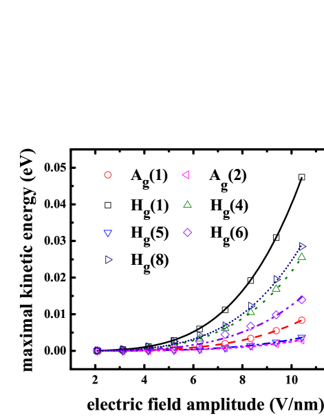
Figure 2: Maximum kinetic energy of $A_{g}(1)$, $A_{g}(2)$, $H_{g}(1)$, $H_{g}(4)$, $H_{g}(5)$, $H_{g}(6)$ and $H_{g}(8)$ modes of C₆₀ responding to $0.69$ eV laser pulses when the FWHM pulse duration $\tau$ is fixed at $12$ fs and the electric field amplitude $\mathcal{E}_{0}$ is varied. Here, and in the subsequent figures, each point represents a DFT-based SERID simulation and each curve has the form predicted by Eq. (7), with no adjustable parameters except the effective polarizability parameter $\alpha_{k}^{\prime}$, which is determined by a least-squares fit.

When $\mathcal{E}_{0}$ is fixed, on the other hand, $K_{k}^{\mathrm{max}}$ is predicted to be proportional to the square of the function involving $r_{k}$ in Eq. (7), and is maximal when $r_{k}\approx 0.84$. Figure 3 shows, for example, that the $H_{g}(8)$ mode in C₆₀ dominates for $2\tau<23.4$ fs, and the $H_{g}(1)$ mode for $2\tau>23.4$ fs, in agreement with the analytical model of Eqs. (2)-(3), and in qualitative agreement with other simulations Zhang and experiment  Dexheimer1993 ; Hohmann1994 ; Bhardwaj2003 ; Boyle2005 ; Larrmann2007 .

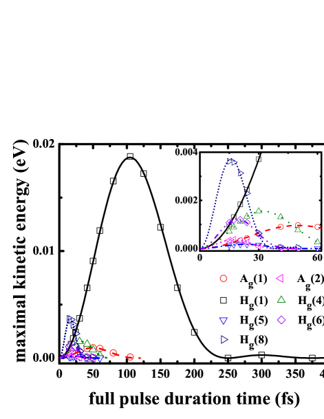
Figure 3: Maximum kinetic energy for the 7 prominent modes of C₆₀ responding to $0.69$ eV laser pulses when $\mathcal{E}_{0}$ is fixed at $5.0$ V/nm and the full pulse duration time $2\tau$ is varied. The agreement between the general model of Eqs. (2)-(3) (curves) and the density-functional-based simulations of Eqs. (8)-(11) (points) is remarkable.

In Fig. 3, the agreement between the predictions of the analytical model (curves) and the completely independent DFT-based simulations (points) is truly remarkable. The only adjustable parameter for each curve is the effective polarizability parameter $\alpha_{k}^{\prime}$.

There is similarly remarkable agreement for the carbon nanotube, as can be seen in Fig. 4. In this case, two photon energies $\hbar\omega$ were used: $0.8$ eV and $2.0$ eV, which are respectively below and above the excitation gap of $1.56$ eV for this model nanotube, as discussed above. Figure 4 shows the results for the maximum kinetic energy $K_{k}^{\mathrm{max}}$ of the one prominent mode observed in this case. (Recall that the polarization vector for the pulse was chosen to point across the nanotube, so that only radial modes should be directly excited, and this is a severe constraint for the small (3,3) nanotube, as is also observed in experiment Hulman2004 .) The panels in Fig. 4 correspond to: (a) $\hbar\omega=0.8$ eV, $\tau=76$ fs; (b) $\hbar\omega=0.8$ eV, $\mathcal{E}_{0}=9.66$ V/nm; (c) $\hbar\omega=2.0$ eV, $\tau=76$ fs; (d) $\hbar\omega=2.0$ eV, $\mathcal{E}_{0}=9.66$ V/nm. It is interesting that the analytical model still works in this case even for above-the-gap excitation, but we find less satisfactory agreement for C₆₀, and certainly do not expect the model of Eq. (3) to be generally valid when there is a substantial population of electrons in excited states at the end of the pulse. In this case other effects will ordinarily be of dominant importance Dresselhaus-1992 ; Torralva2001 .

Figure 4: Maximum kinetic energy of $E_{g}$ mode for (3,3) carbon nanotube, excited by a $0.8$ eV laser pulse (a) when $\tau$ is fixed at $76$ fs and $\mathcal{E}_{0}$ is varied and (b) when $\mathcal{E}_{0}$ is fixed at $9.66$ V/nm and $\tau$ is varied. Panels (c) and (d) are the corresponding results for a pulse with a photon energy of $2.0$ eV.

As mentioned above, the electronic response in the DFT-based simulations can be characterized by an effective polarizability parameter $\alpha_{k}^{\prime}$ if one fits Eq. (7) to the results of the simulations. If the model leading to Eq. (7) is in fact consistent with the detailed simulations, then the values obtained when (a) varying the electric field amplitude $\mathcal{E}_{0}$ at constant (FWHM) pulse duration $\tau$ and (b) varying $\tau$ at constant $\mathcal{E}_{0}$ should also be reasonably consistent. Table 1 shows the results for all of the prominent Raman-active modes. The two procedures do lead to generally consistent values, with the differences for the $A_{g}(2)$, $H_{g}(6)$, and $H_{g}(8)$ modes presumably arising from their short periods, so that the approximation of averaging out the $\omega$ oscillations in Eq. (2) is not valid. However, the prediction regarding optimum pulse duration works even for these modes, as can be seen in Fig. 3.

Table 1: For each of the prominent modes observed in the response of C₆₀ and the (3,3) carbon nanotube, the values of the effective $\alpha_{k}^{\prime}$ were obtained through the procedures designated (a) and (b) in the text. In procedure (a), $\mathcal{E}_{0}$ was varied while the (FWHM) duration $\tau$ was fixed at $12$ fs, for C₆₀, or $76$ fs, for the nanotube. In procedure (b), $\tau$ was varied while $\mathcal{E}_{0}$ was fixed at $5.0$ V/nm, for C₆₀, or $9.66$ V/nm, for the nanotube. The nanotube was also subjected to $2.0$ eV pulses, and the effective values of $\alpha_{k}^{\prime}$ obtained through both procedures are again shown.

	mode	$\alpha_{k}^{\prime}$ (a)	$\alpha_{k}^{\prime}$ (b)
carbon nanotube	Eg	$7.578\times 10^{-4}$	$7.496\times 10^{-4}$
C60	A${}_{g}(1)$	$4.416\times 10^{-4}$	$4.505\times 10^{-4}$
	Ag(2)	$6.248\times 10^{-4}$	$8.102\times 10^{-4}$
	Hg(1)	$9.668\times 10^{-4}$	$9.516\times 10^{-4}$
	Hg(4)	$8.978\times 10^{-4}$	$8.884\times 10^{-4}$
	Hg(5)	$4.482\times 10^{-4}$	$4.294\times 10^{-4}$
	Hg(6)	$1.127\times 10^{-3}$	$1.316\times 10^{-3}$
	Hg(8)	$2.376\times 10^{-3}$	$2.788\times 10^{-3}$
nanotube, above gap $\hbar\omega$	Eg	$1.314\times 10^{-4}$	$1.307\times 10^{-4}$

It has long been suspected that there might be an optimum pulse duration. For example, in Ref. Zhang the pulse envelope was assumed to have a Gaussian form: $\left|\mathcal{E}(t)\right|^{2}=A\exp\left(-2t^{2}/\bar{\tau}^{2}\right)\cos^{2}\left(\omega t\right)$ (with a slight change in notation). Simulations were then performed with a model that essentially lies between the analytical model of Eqs. (2)-(3) and our much more extensive density-functional-based simulations, defined by Eqs. (8)-(11). It was found that the optimum value of $\bar{\tau}$ was about $T/3.4$. The corresponding FWHM duration then has an optimum value $\tau=\sqrt{2\ln 2}\;\bar{\tau}\approx 0.35\,T$. In both our general model and DFT-based simulations, on the other hand, the optimal FWHM pulse duration is found to be given by $\tau\approx 0.42\,T$. Both results seem to be consistent with the existing experiments Dexheimer1993 ; Hohmann1994 ; Bhardwaj2003 ; Boyle2005 ; Larrmann2007 , and both are larger than the naïve prediction of $\tau=0.25\,T$. In our result, the reason appears to be the phase lag apparent in Eq. (5).

It should be emphasized that our result of $\tau\approx 0.42\,T$ is for the maximum response of this mode when the intensity of the laser pulse is kept fixed while the duration is varied. On the other hand, if the fluence is instead held fixed (while $\tau$ is varied), Eqs. (5) and (7) are changed to

$$Q_{k}(t)=\frac{\alpha_{k}^{\prime}W}{\omega_{k}\pi c\epsilon_{0}}\frac{\sin(r_{k}\pi)}{r_{k}(1-r_{k}^{2})}\sin(\omega_{k}t-r_{k}\pi)\quad,\quad t\geq 2\tau$$ (12)

and

$$E_{k}=\frac{1}{2}\left[\frac{\alpha_{k}^{\prime}W}{\pi c\epsilon_{0}}\frac{\sin\left(r_{k}\pi\right)}{r_{k}(1-r_{k}^{2})}\right]^{2}\quad,\quad t\geq 2\tau$$ (13)

where

$$W=\frac{c\epsilon_{0}}{4}\mathcal{E}_{0}^{2}\tau$$ (14)

is the energy in the pulse. If $W$ is held constant, the maximum in Eq. (13) is achieved as $r_{k}\rightarrow 0$:

$$E_{k}\left(0\right)=\frac{1}{2}\left[\frac{\alpha_{k}^{\prime}W}{c\epsilon_{0}}\right]^{2}$$ (15)

so that

$$\frac{E_{k}\left(\tau\right)}{E_{k}\left(0\right)}=\left[\frac{\sin\left(r_{k}\pi\right)}{\pi r_{k}(1-r_{k}^{2})}\right]^{2}\;.$$ (16)

Then $r_{k}=0.84$ gives $E_{k}\left(0.42\,T\right)/E_{k}\left(0\right)=0.385$. However, Eq. (15) holds for all modes, so there is no relative enhancement of any preferred mode.

It should also be emphasized that the success of the simple analytical model of Eq. (3) results from the fact that the additional effects described below Eq. (3) are not very important for the pulse intensities, time durations, and systems considered here. The various effects omitted in the model will lead to richer (or messier) behavior in regimes where nonlinear effects, anharmonicity, damping, etc. become comparable in importance to the lowest-order effects included in the model. In future studies with density-functional-based simulations based on Eqs. (8)-(11) it may be interesting to sort out the influence of the higher-order effects.

Finally, as emphasized below Eq. (1), the present results are for $\hbar\omega$ off resonance, in contrast to those of e.g. Refs. Torralva2001 and smith-1996 . In particular, Smith and Cina considered pulses whose central frequencies are near resonance with an electronic transition, in a model with two electronic levels and one vibrational degree of freedom. They found that the momentum increment (for the nuclei) falls off less rapidly with increasing offset (from resonance) than does the population loss (from the electronic ground state), and they presented a rather complex strategy for optimizing the various parameters for these “preresonant” pulses. The work of this group and others is thus complementary to that of the present paper.

In summary, we find remarkable agreement between the general model of Eqs. (2)-(3) and the detailed DFT-based simulations based on Eqs. (8)-(11) for C₆₀ and a carbon nanotube. At fixed pulse intensity, both of these approaches predict maximum excitation of a Raman-active vibrational mode with period $T$ when the pulse has an FWHM duration $\tau\approx 0.42\,T$.

- (1) S. De Silvestri, J. G. Fujimoto, E. P. Ippen, E. B. Gamble Jr., L. R. Williams, and K. A. Nelson, Chem. Phys. Lett. 116, 146 (1985).
- (2) Y.-X. Yan, E. B. Gamble Jr., and K. A. Nelson, J. Chem. Phys. 83, 5391 (1985).
- (3) A. M. Weiner, D. E. Leaird, G. P. Wiederrecht, and K. A. Nelson, Science 247, 1317 (1990).
- (4) H. J. Zeiger, J. Vidal, T. K. Cheng, E. P. Ippen, G. Dresselhaus, and M. S. Dresselhaus, Phys. Rev. B 45, 768 (1992).
- (5) C. J. Bardeen, Q. Wang, and C. V. Shank, Phys. Rev. Lett. 75, 3410 (1995).
- (6) A. Nazarkin and G. Korn, Phys. Rev. A 58, R61 (1998).
- (7) A. Nazarkin, G. Korn, M. Wittmann, and T. Elsaesser, Phys. Rev. Lett. 83, 2560 (1999).
- (8) R. A. Bartels, S. Backus, M. M. Murnane, and H. C. Kapteyn, Chemical Physics Letters 374, 326 (2003).
- (9) S.-Y. Lee, D. Zhang, D. W. McCamant, P. Kukura, and R. A. Mathies, J. Chem. Phys. 121, 3632 (2004).
- (10) H. Niikura, D. M. Villeneuve, and P. B. Corkum, Phys. Rev. Lett. 92, 133002 (2004).
- (11) B. Torralva, T. A. Niehaus, M. Elstner, S. Suhai, Th. Frauenheim, and R. E. Allen, Phys. Rev. B 64, 153105 (2001).
- (12) G. P. Zhang and T. F. George, Phys. Rev. Lett. 93, 147401 (2004); Phys. Rev. B 73, 035422 (2006).
- (13) U. Banin, A. Bartana, S. Ruhman, and R. Kosloff, J. Chem. Phys. 101, 8461 (1994).
- (14) T. J. Smith and J. A. Cina, J. Chem. Phys. 104, 1272 (1996).
- (15) T. E. Stevens, J. Hebling, J. Kuhl, and R. Merlin, Physica Status Solidi (b) 215, 81 (1999).
- (16) H. Rabitz, R. de Vivie-Riedle, M. Motzkus, and K. Kompa, Science 288, 824 (2000).
- (17) T. C. Weinacht, R. Bartels, S. Backus, P. H. Bucksbaum, B. Pearson, J. M. Geremia, H. Rabitz, H. C. Kapteyn, and M. M. Murnane, Chem. Phys. Lett. 344, 333 (2001).
- (18) R. A. Bartels, T. C. Weinacht, S. R. Leone, H. C. Kapteyn, and M. M. Murnane, Phys. Rev. Lett. 88, 033001(2002).
- (19) A. Assion, T. Baumert, M. Bergt, T. Brixner, B. Kiefer, V. Seyfried, M. Strehle, and G. Gerber, Science 282, 919 (1998).
- (20) K. T. Tsen, S.-W. D. Tsen, C.-L. Chang, C.-F. Hung, T. C. Wu, and J. G. Kiang, Virol. J. 4, 50 (2007).
- (21) K. T. Tsen, S.-W. D. Tsen, O. F. Sankey, and J. G. Kiang, J. Phys.: Condens. Matter 19, 472201 (2007).
- (22) E. C. Dykeman and O. F Sankey, Phys. Rev. Lett. 100, 028101 (2008).
- (23) E. C. Dykeman and O. F Sankey, J. Phys.: Condens. Matter 21, 505102 (2009).
- (24) S. L. Dexheimer, D. M. Mittleman, R. W. Schoenlein, W. Vareka, X. -D. Xiang, A. Zettl, and C. V. Shank, in Ultrafast Phenomena VIII, edited by J. L. Martin, A. Migus, G. A. Mourou, and A. H. Zewail, (Springer-Verlag, Berlin, 1993) p. 81.
- (25) H. Hohmann, C. Callegari, S. Furrer, D. Grosenick, E. E. B. Campbell, and I. V. Hertel , Phys. Rev. Lett. 73, 1919 (1994).
- (26) M. Boyle, T. Laarmann, K. Hoffmann, M. Hedén, E. E. B. Campbell, C. P. Schulz, and I. V. Hertel, Eur. Phys. J. D 36, 339 (2005).
- (27) T. Laarmann, I. Shchatsinin, A. Stalmashonak, M. Boyle, N. Zhavoronkov, J. Handt, R. Schmidt, C. P. Schulz, and I. V. Hertel, Phys. Rev. Lett. 98, 058302 (2007).
- (28) V. R. Bhardwaj, P. B. Corkum, and D. M. Rayner, Phys. Rev. Lett. 91, 203004 (2003).
- (29) Carbon Nanotubes, Advanced Topics in the Synthesis, Structure, Properties and Applications, edited by A. Jorio, G. Dresselhaus, and M. S. Dresselhaus (Springer, Berlin, 2008).
- (30) H. J. Liu and C. T. Chan, Phys. Rev. B 66, 115416 (2002).
- (31) M. Hulman, H. Kuzmany, O. Dubay, G. Kresse, L. Li, Z. K. Tang, P. Knoll, and R. Kaindl, Carbon 42, 1071 (2004).
- (32) J. S. Graves and R. E. Allen, Phys. Rev. B 58, 13627 (1998).
- (33) Y. R. Shen and N. Bloembergen, Phys. Rev. 137, A1787 (1965).
- (34) D. Porezag, Th. Frauenheim, Th. Köhler, G. Seifert, and R. Kaschner, Phys. Rev. B 51, 12947 (1995).
- (35) G. Seifert, D. Porezag, and Th. Frauenheim Int. J. Quantum Chem. 58, 185 (1996). See http://www.dftb.org and http://www.dftb-pluse.info for the currently best versions.
- (36) R. E. Allen, Phys. Rev. B 78, 064305 (2008) and references therein.