AdS/CFT on the brane

Abstract

It is widely recognized that the AdS/CFT correspondence is a useful tool to study strongly coupled field theories. On the other hand, Randall-Sundrum (RS) braneworld models have been actively discussed as a novel cosmological framework. Interestingly, the geometrical set up of braneworlds is quite similar to that in the AdS/CFT correspondence. Hence, it is legitimate to seek a precise relation between these two different frameworks. In this lecture, I will explain how the AdS/CFT correspondence is related to the RS braneworld models. There are two different versions of RS braneworlds, namely, the single-brane model and the two-brane model. In the case of the single-brane model, we reveal the relation between the geometrical and the AdS/CFT correspondence approach using the gradient expansion method. It turns out that the high energy and the Weyl term corrections found in the geometrical approach correspond to the CFT matter correction found in the AdS/CFT correspondence approach. In the case of two-brane system, we also show that the AdS/CFT correspondence plays an important role in the sense that the low energy effective field theory can be described by the conformally coupled scalar-tensor theory where the radion plays the role of the scalar field. We also discuss dilatonic braneworld models from the point of view of the AdS/CFT correspondence.

1 Introduction

It is believed that string theory is a candidate of the unified theory of everything. Remarkably, string theory can be consistently formulated only in 10 dimensions sodPolchinski . This fact requires a mechanism to fill the gap between our real world and the higher dimensions. Conventionally, the extra dimensions are considered to be compactified to a small compact space of the order of the Planck scale. However, recent developments of superstring theory invented a new idea, the so-called braneworld where matter resides on the hypersurface in higher dimensional spacetime sodHorava:1995qa ; sodHorava:1996ma ; sodLukas:1998yy ; sodAntoniadis:1998ig ; sodArkaniHamed:1998nn ( see also earlier independent works sodAkama:1982jy ; sodRubakov:1983bb ). This hypersurface is called (mem)brane. This idea originates from D-brane solutions in string theory. Interestingly, the D-brane solution also gives rise to the AdS/CFT correspondence which claims that classical gravity in an anti-de Sitter(AdS) spacetime is equivalent to a strongly coupled conformally invariant field theory (CFT). Since the origin is the same, braneworlds and the AdS/CFT correspondence may be related to each other. In particular, Randall and Sundrum (RS) braneworld models sodRS1 ; sodRS2 have a similar geometrical setup to that in the AdS/CFT correspondence. Hence, in this lecture, I will try to reveal relations between the AdS/CFT correspondence and RS braneworld models sodKanno:2004ns .

The method we will use is the gradient expansion method. Physically, it is a low energy expansion method. Historically, the method has been used in the cosmological context sodtomita ; sodSalopek:1992kk ; sodComer ; sodSII . In particular, it is known to be useful for analyzing the evolution of cosmological perturbations during inflation. Since the AdS spacetime can be regarded as the inflating universe in the spatial direction, the gradient expansion method is also expected to be useful in the AdS spacetime. First, by utilizing the gradient expansion method, we approximately solve Einstein equations in the bulk. Then, the junction conditions at the brane give the effective equations of motion on the brane. Thus, we can understand the low energy physics in the braneworld. The similar but slightly different method is also used in the AdS/CFT correspondence. We will identify a concrete relation between the geometrical and the AdS/CFT correspondence approach by detailed comparison. The difference shows up when we consider two brane systems. Indeed, we do not have the conventional AdS/CFT correspondence for the two-brane system. Instead, we have a conformally coupled radion on the brane which reflects the conformal symmetry of the theory. This observation is useful for understanding why brane inflation suffers from the eta problem. It is apparent that the gradient expansion method can be applicable to various braneworld models. Moreover, as we will see, the gradient expansion method provides a unified view of branworlds and a useful tool to make cosmological predictions.

The organization of this lecture is as follows: In section 2, we introduce RS models and derive the effective Friedman equation on the brane. Here, two important corrections, i.e., the dark radiation and the high energy corrections, are identified. This sets our starting point. In section 3, we review two different views from the brane, namely, the AdS/CFT correspondence and the geometrical holography. These two frameworks give us a complementary picture of the braneworlds. In section 4, we present key questions to make our concerns manifest. In section 5, we review the gradient expansion method. In sections 6 and 7, we apply the gradient expansion method to the single-brane model and to the two-brane model, respectively. We obtain the effective theory for both cases. In section 8, we give answers to the key questions. This completes explanation of relations between the AdS/CFT correspondence and RS braneworld models. In section 9, we extend our analysis to models with a bulk scalar field. Since the presence of bulk fields would break the conformal invariance, it is interesting to consider dilatonic braneworlds in conjunction with the AdS/CFT correspondence. The final section is devoted to the conclusion.

2 Braneworlds in AdS spacetime

In this section, we will introduce RS braneworld models. We will derive the effective Friedmann equation and identify the effects of extra-dimensions. In this lecture, we will concentrate on cosmology although we can apply the results to black hole physics.

2.1 RS Models

Randall and Sundrum proposed a simple model where a four-dimensional brane with the tension $\sigma$ is embedded in the five-dimensional asymptotically anti-de Sitter (AdS) bulk with a curvature scale $\ell$. This single-brane model is described by the action sodRS2

$$S = {1\over 2\kappa^{2}}\int d^{5}x\sqrt{-g}\left({\cal R}+{12\over\ell^{2}}\right)-\sigma\int d^{4}x\sqrt{-h}+\int d^{4}x\sqrt{-h}{\cal L}_{\rm matter}\ ,$$ (1)

where ${\cal R}$ and $\kappa^{2}$ are the scalar curvature and gravitational constant in five-dimensions, respectively. We impose $Z_{2}$ symmetry on this spacetime, with the brane at the fixed point. The matter ${\cal L}_{\rm matter}$ is confined to the brane. Throughout this lecture, $h_{\mu\nu}$ represents the induced metric on the brane. Remarkably, the internal dimension is non-compact in this model. Hence, we do not have to care about the stability problem. The basic equations consist of the equations of motion in the bulk and junction conditions at the brane position due to the presence of the brane. Alternatively, the basic equations can be regarded as the 5-dimensional Einstein equations with singular sources. Let us recall the 4-dimensional components of 5-dimensional Einstein tensor can be expressed by

$$\overset{(5)}{G}{}_{\mu\nu} = \overset{(4)}{G}{}_{\mu\nu}+{\cal L}_{n^{\mu}}\left[K_{\mu\nu}-g_{\mu\nu}K\right]+\cdots\ ,$$ (2)

where ${\cal L}_{n^{\mu}}$ denotes the Lie derivative along the unit normal vector to the brane, $n^{\mu}$. Here, we defined the extrinsic curvature by

$$K_{\mu\nu}=-\left(\delta_{\mu}^{\rho}-n_{\mu}n^{\rho}\right)\nabla_{\rho}n_{\nu}\ .$$ (3)

By integrating Einstein equations along the normal to the brane, we obtain the jump of the extrinsic curvature $(K^{+}_{\mu\nu}-g_{\mu\nu}K^{+})-(K^{-}_{\mu\nu}-g_{\mu\nu}K^{-})$ from the left hand side and the total energy momentum tensor on the brane from the right hand side due to the delta function sources. Thus, taking into account the $Z_{2}$ symmetry $K_{\mu\nu}\equiv K^{+}_{\mu\nu}=-K^{-}_{\mu\nu}$, we obtain the junction conditions

$$\left[K^{\mu}{}_{\nu}-\delta^{\mu}_{\nu}K\right]\Big{|}_{\rm at\ the\ brane}={\kappa^{2}\over 2}\left(-\sigma\delta^{\mu}_{\nu}+T^{\mu}{}_{\nu}\right)\ .$$ (4)

Here, $T_{\mu\nu}$ represents the energy-momentum tensor of the matter.

Originally, they proposed the two-brane model as a possible solution of the hierarchy problem sodRS1 . The action reads

$$S = {1\over 2\kappa^{2}}\int d^{5}x\sqrt{-g}\left({\cal R}+{12\over\ell^{2}}\right)$$ (5)

$$\quad-\sum_{i=\oplus,\ominus}\sigma_{i}\int d^{4}x\sqrt{-h_{i}}+\sum_{i=\oplus,\ominus}\int d^{4}x\sqrt{-h}{\cal L}_{\rm matter}^{i}\ ,$$

where $\oplus$ and $\ominus$ represent the positive and the negative tension branes, respectively. In principle, one can consider multiple-branes although they are not discussed in this lecture.

2.2 Cosmology

The homogeneous cosmology of the single-brane model is easy to analyze sodBrax:2004xh . Because of the Birkoff theorem due to the symmetry on the brane, it is sufficient to consider AdS black hole spacetime:

$$ds^{2}=-h(r)dt^{2}+\frac{dr^{2}}{h(r)}+r^{2}\left[d\chi^{2}+f_{k}^{2}(\chi)\left(d\theta^{2}+\sin^{2}\theta d\phi^{2}\right)\right]\ ,$$ (6)

where

$$f_{k}=\left\{\begin{array}[]{cc}\sin\chi&{\rm for}\ k=1\\ \chi&{\rm for}\ k=0\\ \sinh\chi&{\rm for}\ k=-1\end{array}\right.$$ (10)

and

$$h(r)=k-\frac{M}{r^{2}}+\frac{r^{2}}{\ell^{2}}\ .$$ (11)

Note that $M$ is the mass of the black hole, $k$ is the curvature of the horizon and $\ell$ is the AdS curvature radius. Suppose the brane is moving in this spacetime with a trajectory $t=t(\tau)\ ,r=a(\tau)$, where $\tau$ is a proper time of the brane (see Fig.1). The induced metric on the brane becomes

$$ds_{ind}^{2}=-d\tau^{2}+a^{2}(\tau)\left[d\chi^{2}+f_{k}^{2}(\chi)\left(d\theta^{2}+\sin^{2}\theta d\phi^{2}\right)\right]\ .$$ (12)

This is nothing but the Friedman-Robertson-Walker spacetime where $a$ is the scale factor. The motion of the brane cannot be arbitrary. It is constrained by the junction condition:

$$K^{\chi}{}_{\chi}=-\frac{\kappa^{2}\sigma}{6}-\frac{\kappa^{2}}{2}\left[T^{\chi}{}_{\chi}-\frac{1}{3}T\right]\ ,$$ (13)

where $K^{\chi}{}_{\chi}$, $T^{\chi}{}_{\chi}$, $T$ are a $\chi\chi$ component of the extrinsic curvature, a $\chi\chi$ component and the trace part of the energy momentum tensor of matter on the brane, respectively.

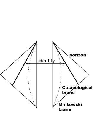
Figure 1: The Minkowski brane represented by the dotted line is a static brane in the Poincare coordinate system of the AdS spacetime. While, the cosmological brane represented by the thick line is moving in the bulk. The motion of the brane induces the expansion of the brane universe. The Cauchy horizon of AdS spacetime corresponds to the big-bang singularity. In the case of AdS-Schwarzschild spacetime, the horizon should be the past horizon of the black hole. The big bang is located beyound the horizon.

From the normalization condition $n^{\mu}n_{\mu}=1$ of the unit normal vector $n^{\mu}=(-\dot{a},\dot{t})$, we obtain

$$\dot{t}=\sqrt{\frac{1}{h(a)}+\frac{\dot{a}^{2}}{h^{2}(a)}}\ .$$ (14)

Here, the dot is a derivative with respect to the proper time $\tau$. Now, one can calculate $K_{\chi\chi}$ as

$$K_{\chi\chi}=-\nabla_{\chi}n_{\chi}=-\partial_{\chi}n_{\chi}+\Gamma^{r}_{\chi\chi}=-\frac{1}{2}n^{r}\frac{\partial}{\partial\chi}g_{\chi\chi}\ .$$ (15)

Hence, from Eqs.(13), (14) and (15), we have an equation

$$\frac{1}{a}\sqrt{h(a)+\dot{a}^{2}}=\frac{\kappa^{2}}{6}\left(\sigma+\rho\right)\ .$$ (16)

Thus, we get

$$\frac{k}{a^{2}}-\frac{M}{a^{4}}+\ell^{2}+\frac{\dot{a}^{2}}{a^{2}}=\frac{\kappa^{4}}{36}\left(\sigma+\rho\right)^{2}\ ,$$ (17)

or

$$H^{2}=\frac{\kappa^{4}\sigma^{2}}{36}-\frac{1}{\ell^{2}}+\frac{\kappa^{4}\sigma}{18}\rho-\frac{k}{a^{2}}+\frac{M}{a^{4}}+\frac{\kappa^{4}}{36}\rho^{2}\ .$$ (18)

By setting $\kappa^{2}\sigma\ell=6$, we finally derived the effective Friedmann equation as sodBinetruy:1999hy ; sodKraus:1999it ; sodFlanagan:1999cu ; sodIda:1999ui ; sodKaloper:1999sm

$$H^{2}=-\frac{k}{a^{2}}+{\kappa^{2}\over 3\ell}\rho+\frac{M}{a^{4}}+\frac{\kappa^{4}}{36}\rho^{2}\ ,$$ (19)

where $H=\dot{a}/a$ is the Hubble parameter. The Newton’s constant can be identified as $8\pi G_{N}=\kappa^{2}/\ell$. The curvature of the horizon $k$ corresponds spatial curvature of the universe. The black hole mass $M$ is referred to as the dark radiation sodMukohyama:1999qx which is not real radiation fluid but a reflection of the bulk geometry. This effect exists even in the low energy regime. The last term represents the high energy effect of the braneworld sodMaartens:2003tw .

As to the two-brane model, the same effective Friedmann equation (19) can be expected on each brane because the above equation (19) has been deduced without referring to the bulk equations of motion.

Given this cosmological background, it is natural to investigate cosmological perturbation in the braneworld sodMaartens:2004yc . In the case of the single-brane model, it is shown that the gravity in Minkowski brane is localized on the brane in spite of the noncompact extra dimension. Consequently, it turned out that the conventional linearized Einstein equation approximately holds at scales large compared with the curvature scale $\ell$. It should be stressed that this result can be attained by imposing the outgoing boundary conditions. It turns out that this is also true in the cosmological background sodKoyama:2000cc .

In the case of the two-brane model, Garriga and Tanaka analyzed linearized gravity and have shown that the gravity on the brane behaves as the Brans-Dicke theory at low energy sodGT . Thus, the conventional linearized Einstein equations do not hold even on scales large compared with the curvature scale $\ell$ in the bulk. Charmousis et al. have clearly identified the Brans-Dicke field as the radion mode sodCR .

In the end, we would like to know how nonlinear gravity in the braneworld is deviated from the conventional Einstein gravity. A partial answer will be given in the following sections.

3 View from the brane

In the previous section, we have considered an isotropic and homogeneous universe and seen that the effective Friedmann equation on the brane can be regarded as the conventional Friedmann equation with two kind of corrections, i.e., the dark radiation and high-energy corrections. Here, we review two different approaches to extend the above result to more general cases.

3.1 AdS/CFT Correspondence

Let us start with the AdS/CFT correspondence sodmalda ; sodGubser:1998bc ; sodWitten:1998qj . After solving the equations of motion in the bulk with the boundary value fixed and substituting the solution $g_{\rm cl}$ into the 5-dimensional Einstein-Hilbert action $S_{\rm 5d}$, we obtain the effective action for the boundary field $h=g_{\rm cl}|_{\rm boundary}$. The statement of the AdS/CFT correspondence is that the resultant effective action can be equated with the partition functional of some conformally invariant field theory (CFT), namely

$$\exp\left[iS_{\rm 5d}[g_{\rm cl}]\right]\approx<\exp\left[i\int h{\cal O}\right]>_{\rm CFT}\ ,$$ (20)

where ${\cal O}$ is the field in CFT. In the right hand side, $h$ should be interpreted as a source field. This action must be defined at the AdS infinity where the conformal symmetry exists as the asymptotic symmetry. Hence, there exist infrared divergences which must be subtracted by counter terms. Thus, the correct formula becomes

$$\exp\left[iS_{\rm 5d}[g_{\rm cl}]+iS_{\rm ct}\right]=<\exp\left[i\int h{\cal O}\right]>_{\rm CFT}\ ,$$ (21)

where we added the counter terms

$$S_{\rm ct}=S_{\rm brane}-S_{\rm 4d}-[~{}R^{2}{\rm terms}~{}]\ ,$$ (22)

where $S_{\rm brane}$ and $S_{4d}$ are the brane action and the 4-dimensional Einstein-Hilbert action, respectively. Here, the higher curvature terms $[R^{2}{\rm terms}]$ should be understood symbolically.

In the case of the braneworld, the brane acts as the cutoff. Therefore, there is no divergences in the above expressions. In other words, no counter term is necessary. We can regard the above relation as the definition of the “cut off” CFT. Thus, we can freely rearrange the terms as follows

$$S_{\rm 5d}+S_{\rm brane}=S_{\rm 4d}+S_{\rm CFT}+[~{}R^{2}{\rm terms}~{}]\ ,$$ (23)

where we have defined

$$\exp iS_{\rm CFT}\equiv<\exp\left[i\int h{\cal O}\right]>_{\rm CFT}\ .$$ (24)

This tells us that the brane models can be described as the conventional Einstein theory with the cutoff CFT and higher order curvature terms soddeHaro:2000wj ; sodads1 ; sodads2 ; sodads3 . In terms of the equations of motion, the AdS/CFT correspondence reads

$$\overset{(4)}{G}{}_{\mu\nu}={\kappa^{2}\over\ell}\left(T_{\mu\nu}+T^{\rm CFT}_{\mu\nu}\right)+[~{}R^{2}{\rm terms}~{}]\ ,$$ (25)

where the $R^{2}$ terms represent the higher order curvature terms and $T^{CFT}_{\mu\nu}$ denotes the energy-momentum tensor of the cutoff version of conformal field theory. When we apply this result to cosmology, we see CFT corresponds to the dark radiation in the braneworld and the higher curvature terms can be reduced to the high-energy corrections.

3.2 Geometrical Holography

Here, let us review the geometrical approach sodShiMaSa . In the Gaussian normal coordinate system:

$$ds^{2}=dy^{2}+g_{\mu\nu}(y,x^{\mu})dx^{\mu}dx^{\nu}\ ,$$ (26)

we can write the 5-dimensional Einstein tensor $\overset{(5)}{G}{}_{\mu\nu}$ in terms of the 4-dimensional Einstein tensor $\overset{(4)}{G}{}_{\mu\nu}$ and the extrinsic curvature as

$$\overset{(5)}{G}{}_{\mu\nu} = \overset{(4)}{G}{}_{\mu\nu}+K_{\mu\nu,y}-g_{\mu\nu}K_{,y}-KK_{\mu\nu}+2K_{\mu\lambda}K^{\lambda}{}_{\nu}$$ (27)

$$\qquad+{1\over 2}g_{\mu\nu}\left(K^{2}+K^{\alpha}{}_{\beta}K^{\beta}{}_{\alpha}\right)$$

$$= {6\over\ell^{2}}g_{\mu\nu}\ ,$$

where we have introduced the extrinsic curvature

$$K_{\mu\nu}=-{1\over 2}g_{\mu\nu,y}\ ,$$ (28)

and the last equality comes from the 5-dimensional Einstein equations. On the other hand, the Weyl tensor in the bulk can be expressed as

$$C_{y\mu y\nu}=K_{\mu\nu,y}-g_{\mu\nu}K_{,y}+K_{\mu}{}^{\lambda}K_{\lambda\nu}+g_{\mu\nu}K^{\alpha\beta}K_{\alpha\beta}-\frac{3}{\ell^{2}}g_{\mu\nu}\ .$$ (29)

Now, one can eliminate $K_{\mu\nu,y}-g_{\mu\nu}K_{,y}$ from (27) using (29) and obtain

$$\overset{(4)}{G}{}_{\mu\nu} = -C_{y\mu y\nu}+KK_{\mu\nu}-K_{\mu\lambda}K^{\lambda}{}_{\nu}$$ (30)

$$\qquad-{1\over 2}g_{\mu\nu}\left(K^{2}-K^{\alpha}{}_{\beta}K^{\beta}{}_{\alpha}\right)+{3\over\ell^{2}}g_{\mu\nu}\ .$$

Taking into account the $Z_{2}$ symmetry, we also obtain the junction conditions

$$\left[K^{\mu}{}_{\nu}-\delta^{\mu}_{\nu}K\right]\Big{|}_{y=0}={\kappa^{2}\over 2}\left(-\sigma\delta^{\mu}_{\nu}+T^{\mu}{}_{\nu}\right)\ .$$ (31)

Here, $T_{\mu\nu}$ represents the energy-momentum tensor of the matter. Evaluating Eq. (30) at the brane and substituting the junction condition into it, we have the “effective” equations of motion

$$\overset{(4)}{G}{}_{\mu\nu}={\kappa^{2}\over\ell}T_{\mu\nu}+\kappa^{4}\pi_{\mu\nu}-E_{\mu\nu}$$ (32)

where we have defined the quadratic of the energy momentum tensor

$$\pi_{\mu\nu}=-{1\over 4}T_{\mu}{}^{\lambda}T_{\lambda\nu}+{1\over 12}TT_{\mu\nu}+{1\over 8}g_{\mu\nu}\left(T^{\alpha\beta}T_{\alpha\beta}-{1\over 3}T^{2}\right)$$ (33)

and the projection of Weyl tensor $C_{y\mu y\nu}$ onto the brane

$$E_{\mu\nu} = C_{y\mu y\nu}|_{y=0}\ .$$

Here, we assumed the relation

$$\kappa^{2}\sigma=\frac{6}{\ell}$$ (34)

so that the effective cosmological constant vanishes.

Because of the traceless property of $E_{\mu\nu}$, when we consider an isotropic and homogeneous universe, it is easy to show that this gives the dark radiation component $\propto 1/a^{4}$. The existence of the high-energy corrections $\propto\rho^{2}$ is apparent in this approach.

The geometrical approach is useful to classify possible corrections to the conventional Einstein equations. One defect of this approach is the fact that the projected Weyl tensor $E_{\mu\nu}$ can not be determined without solving the equations in the bulk.

4 Does AdS/CFT play any role in braneworld?

To make our concerns explicit, we give a sequence of questions. We treat the single-brane model and two-brane model, separately.

4.1 Single-brane model

Is the Einstein theory recovered even in the non-linear regime?

In the case of the linear theory, it is known that the conventional Einstein theory is recovered at low energy. On the other hand, the cosmological consideration suggests the deviation from the conventional Friedmann equation even in the low energy regime. This is due to the dark radiation term. Therefore, we need to clarify when the conventional Einstein theory can be recovered on the brane.

How does the AdS/CFT come into the braneworld?

It was argued that the cutoff CFT comes into the braneworld. However, no one knows what is the cutoff CFT. It is a vague concept at least from the point of view of the classical gravity. Moreover, it should be noted that the AdS/CFT correspondence is a specific conjecture. Indeed, originally, Maldacena conjectured that the supergravity on $AdS_{5}\times S^{5}$ is dual to the four-dimensional ${\cal N}=4$ super Yang-Mills theory sodmalda . Nevertheless, the AdS/CFT correspondence seems to be related to the brane world model as has been demonstrated by several people sodads1 ; sodads2 ; sodads3 ; sodads4 ; sodads5 ; sodads6 ; sodads7 ; sodKiritsis:2005bm ; sodTanaka:2004ig . Hence, it is important to reveal the role of the AdS/CFT correspondence starting from the 5-dimensional general relativity.

How are the AdS/CFT and geometrical approach related?

The geometrical approach gives the effective equations of motion (32)

$$\overset{(4)}{G}{}_{\mu\nu}={\kappa^{2}\over\ell}T_{\mu\nu}+\kappa^{4}\pi_{\mu\nu}-E_{\mu\nu}\ .$$

On the other hand, the AdS/CFT correspondence yields the other effective equations of motion (25)

$$\overset{(4)}{G}{}_{\mu\nu}={\kappa^{2}\over\ell}\left(T_{\mu\nu}+T^{\rm CFT}_{\mu\nu}\right)+[~{}R^{2}{\rm terms}~{}]\ .$$

An apparent difference is remarkable.

It is an interesting issue to clarify how these two descriptions are related. Shiromizu and Ida tried to understand the AdS/CFT correspondence from the geometrical point of view sodSI . They argued that $\pi^{\mu}_{\ \mu}$ corresponds to the trace anomaly of the cutoff CFT on the brane. However, this result is rather paradoxical because there exists no trace anomaly in an odd dimensional brane although $\pi^{\mu}_{\ \mu}$ exists even in that case. Thus, the more precise relation between the geometrical and the AdS/CFT approaches should be given.

Moreover, since both the geometrical and AdS/CFT approaches seem to have their own merit, it would be beneficial to understand the mutual relationship.

4.2 Two-brane model

How is the geometrical approach consistent with the Brans-Dicke picture?

Irrespective of the existence of other branes, the geometric approach gives the same effective equations (32). The effect of the bulk geometry comes into the brane world only through $E_{\mu\nu}$. In this picture, the two-brane system can be regarded as the Einstein theory with some corrections due to the Weyl tensor in the bulk.

On the other hand, the linearized gravity on the brane behaves as the Brans-Dicke theory on scales large compared with the curvature scale $\ell$ in the bulk sodGT . Therefore, the conventional linearized Einstein equations do not hold at low energy.

In the geometrical approach, no radion appears. While, from the linear analysis, it turns out that the system can be described by the Brans-Dicke theory where the extra scalar field is nothing but the radion. How can we reconcile these seemingly incompatible pictures?

What replaces the AdS/CFT correspondence in the two-brane model?

In the single-brane model, there are continuum Kaluza-Klein (KK)-spectrum around the zero mode. They induce the CFT matter in the 4-dimensional effective action. In the two-brane system, the spectrum become discrete and then a mass gap exists. Hence, we can not expect CFT matter on the brane, although KK-modes exist and affect the physics on the brane. So, it is interesting to know if the AdS/CFT correspondence play a role in the two-brane system.

5 Gradient Expansion Method

Our aim in this lecture is to show the gradient expansion method gives the answers to all of the questions presented in the previous section. Here, we review the formalism developed by us  sodKS1 ; sodKS2 ; sodKS3 ; sodKS4 .

We use the Gaussian normal coordinate system (26) to describe the geometry of the brane world. Note that the brane is located at $y=0$ in this coordinate system. Decomposing the extrinsic curvature into the traceless part and the trace part

$$K_{\mu\nu}=\Sigma_{\mu\nu}+{1\over 4}h_{\mu\nu}K\ ,\quad K=-{\partial\over\partial y}\log\sqrt{-g}\ ,$$ (35)

we obtain the basic equations which hold in the bulk;

$$\Sigma^{\mu}{}_{\nu,y}-K\Sigma^{\mu}{}_{\nu}=-\left[\overset{(4)}{R}{}^{\mu}{}_{\nu}-{1\over 4}\delta^{\mu}_{\nu}\overset{(4)}{R}\right]\ ,$$ (36)

$${3\over 4}K^{2}-\Sigma^{\alpha}{}_{\beta}\Sigma^{\beta}{}_{\alpha}=\left[~{}\overset{(4)}{R}~{}\right]+{12\over\ell^{2}}\ ,$$ (37)

$$K_{,y}-{1\over 4}K^{2}-\Sigma^{\alpha\beta}\Sigma_{\alpha\beta}=-{4\over\ell^{2}}\ ,$$ (38)

$$\nabla_{\lambda}\Sigma_{\mu}{}^{\lambda}-{3\over 4}\nabla_{\mu}K=0\ ,$$ (39)

where $\overset{(4)}{R}{}^{\mu}{}_{\nu}$ is the curvature on the brane and $\nabla_{\mu}$ denotes the covariant derivative with respect to the metric $g_{\mu\nu}$. One also has the junction condition

$$\left[K^{\mu}{}_{\nu}-\delta^{\mu}_{\nu}K\right]\Big{|}_{y=0}={\kappa^{2}\over 2}\left(-\sigma\delta^{\mu}_{\nu}+T^{\mu}{}_{\nu}\right)\ .$$ (40)

Recall that we are considering the $Z_{2}$ symmetric spacetime.

The problem now is separated into two parts. First, we will solve the bulk equations of motion with the Dirichlet boundary condition at the brane,

$$g_{\mu\nu}(y=0,x^{\mu})=h_{\mu\nu}(x^{\mu})\ .$$ (41)

After that, the junction condition will be imposed at the brane. As it is the condition for the induced metric $h_{\mu\nu}$, it is naturally interpreted as the effective equations of motion for gravity on the brane.

Along the normal coordinate $y$, the metric varies with a characteristic length scale $\ell$; $g_{\mu\nu,y}\sim g_{\mu\nu}/\ell$. Denote the characteristic length scale of the curvature fluctuation on the brane as $L$; then we have $R\sim g_{\mu\nu}/L^{2}$. For the reader’s reference, let us take $\ell=1$ mm, for example. Then, the relation (34) give the scale, $\kappa^{2}=(10^{8}\ {\rm GeV})^{-3}$ and $\sigma=1\ {\rm TeV}^{4}$. In this lecture, we will consider the low energy regime in the sense that the energy density of matter, $\rho$, on the brane is smaller than the brane tension, ı.e., $\rho/\sigma\ll 1$. In this regime, a simple dimensional analysis

$${\rho\over\sigma}\sim{\ell{\kappa^{2}\over\ell}\rho\over\kappa^{2}\sigma}\sim\left({\ell\over L}\right)^{2}\ll 1$$ (42)

implies that the curvature on the brane can be neglected compared with the extrinsic curvature at low energy. Here, we have used the relation (34) and Einstein’s equation on the brane, $R\sim g_{\mu\nu}/L^{2}\sim\kappa^{2}\rho/\ell$. Thus, the anti-Newtonian or gradient expansion method used in the cosmological context is applicable to our problem sodtomita .

At zeroth order, we can neglect the curvature term. Then we have

$$\overset{(0)}{\Sigma}{}^{\mu}{}_{\nu,y}-\overset{(0)}{K}\overset{(0)}{\Sigma}{}^{\mu}{}_{\nu}=0\ ,$$ (43)

$${3\over 4}\overset{(0)}{K}{}^{2}-\overset{(0)}{\Sigma}{}^{\alpha}{}_{\beta}\overset{(0)}{\Sigma}{}^{\beta}{}_{\alpha}={12\over\ell^{2}}\ ,$$ (44)

$$\overset{(0)}{K}{}_{,y}-{1\over 4}\overset{(0)}{K}{}^{2}-\overset{(0)}{\Sigma}{}^{\alpha\beta}\overset{(0)}{\Sigma}{}_{\alpha\beta}=-{4\over\ell^{2}}\ ,$$ (45)

$$\nabla_{\lambda}\overset{(0)}{\Sigma}{}^{\lambda}{}_{\mu}-{3\over 4}\nabla_{\mu}\overset{(0)}{K}=0\ .$$ (46)

Equation (43) can be readily integrated into

$$\overset{(0)}{\Sigma}{}^{\mu}{}_{\nu}={C^{\mu}{}_{\nu}(x^{\mu})\over\sqrt{-g}}\ ,\quad C^{\mu}{}_{\mu}=0\ ,$$ (47)

where $C^{\mu}{}_{\nu}$ is the constant of integration. Equation (46) also requires $C^{\mu}{}_{\nu|\mu}=0$. If it could exist, it would represent a radiation like fluid on the brane and hence a strongly anisotropic universe. In fact, as we see soon, this term must vanish in order to satisfy the junction condition. Therefore, we simply put $C^{\mu}{}_{\nu}=0$, hereafter. Now, it is easy to solve the remaining equations. The result is

$$\overset{(0)}{K}={4\over\ell}\ .$$ (48)

Using the definition of the extrinsic curvature

$$\overset{(0)}{K}{}_{\mu\nu}=-{1\over 2}{\partial\over\partial y}\overset{(0)}{g}{}_{\mu\nu}\ ,$$ (49)

we get the zeroth order metric as

$$ds^{2}=dy^{2}+b^{2}(y)h_{\mu\nu}(x^{\mu})dx^{\mu}dx^{\nu}\ ,\quad b(y)=e^{-2{y\over\ell}}\ ,$$ (50)

where the tensor $h_{\mu\nu}$ is the induced metric on the brane, which conforms to the boundary condition (41).

From the zeroth order solution, we obtain

$$\left[\overset{(0)}{K}{}^{\mu}{}_{\nu}-\delta^{\mu}_{\nu}\overset{(0)}{K}\right]\Bigg{|}_{y=0}=-{3\over\ell}\delta^{\mu}_{\nu}=-{\kappa^{2}\over 2}\sigma\delta^{\mu}_{\nu}\ .$$ (51)

Then we get the well known relation

$$\kappa^{2}\sigma=6/\ell\ .$$ (52)

Here, we will assume that this relation holds exactly. It is apparent that $C^{\mu}{}_{\nu}$ is not allowed to exist.

The iteration scheme consists in writing the metric $g_{\mu\nu}$ as a sum of local tensors built out of the induced metric on the brane, the number of gradients increasing with the order. Hence, we will seek the metric as a perturbative series

$$g_{\mu\nu}(y,x^{\mu}) = b^{2}(y)\left[h_{\mu\nu}(x^{\mu})+\overset{(1)}{g}{}_{\mu\nu}(y,x^{\mu})+\overset{(2)}{g}{}_{\mu\nu}(y,x^{\mu})+\cdots\right]\ ,$$ (53)

where $b^{2}(y)$ is extracted and we put the Dirichlet boundary condition

$$\overset{(i)}{g}{}_{\mu\nu}(y=0,x^{\mu})=0\ ,$$ (54)

so that $g_{\mu\nu}(y=0,x)=h_{\mu\nu}(x)$ holds at the brane. Other quantities can be also expanded as

$$K^{\mu}{}_{\nu} = {1\over\ell}\delta^{\mu}_{\nu}+\overset{(1)}{K}{}^{\mu}{}_{\nu}+\overset{(2)}{K}{}^{\mu}{}_{\nu}+\cdots$$

$$\Sigma^{\mu}{}_{\nu} = \qquad+\overset{(1)}{\Sigma}{}^{\mu}{}_{\nu}+\overset{(2)}{\Sigma}{}^{\mu}{}_{\nu}+\cdots\ .$$ (55)

In our scheme, in contrast to the AdS/CFT correspondence where the Dirichlet boundary condition is imposed at infinity, we impose it at the finite point $y=0$, the location of the brane. Furthermore, we carefully consider the constants of integration, i.e., homogeneous solutions. These homogeneous solutions are ignored in the calculation of AdS/CFT correspondence. However, they play an important role in the braneworld. Note that the scheme can be applicable to other systems sodShiromizu:2003dr ; sodOnda:2003sj ; sodShiromizu:2003pz ; sodTakahashi:2004ss .

6 Single brane model (RS2)

Now, we will apply the gradient expansion method to the single-brane models and obtain the effective equations on the brane.

6.1 Einstein Gravity at Lowest Order

The next order solutions are obtained by taking into account the terms neglected at zeroth order. At first order, Eqs. (36) - (39) become

$$\overset{(1)}{\Sigma}{}^{\mu}{}_{\nu,y}-{4\over\ell}\overset{(1)}{\Sigma}{}^{\mu}{}_{\nu}=-\left[\overset{(4)}{R}{}^{\mu}{}_{\nu}-{1\over 4}\delta^{\mu}_{\nu}\overset{(4)}{R}\right]^{(1)}\ ,$$ (56)

$${6\over\ell}\overset{(1)}{K}=\left[~{}\overset{(4)}{R}~{}\right]^{(1)}\ ,$$ (57)

$$\overset{(1)}{K}{}_{,y}-{2\over\ell}\overset{(1)}{K}=0\ ,$$ (58)

$$\overset{(1)}{\Sigma}{}_{\mu}{}^{\lambda}{}_{|\lambda}-{3\over 4}\overset{(1)}{K}{}_{|\mu}=0\ .$$ (59)

where the superscript $(1)$ represents the order of the derivative expansion and a stroke $|$ denotes the covariant derivative with respect to the metric $h_{\mu\nu}$. Here, $[\overset{(4)}{R}{}^{\mu}{}_{\nu}]^{(1)}$ means that the curvature is approximated by taking the Ricci tensor of $b^{2}h_{\mu\nu}$ in place of $\overset{(4)}{R}{}^{\mu}{}_{\nu}$. It is also convenient to write it in terms of the Ricci tensor of $h_{\mu\nu}$, denoted $R^{\mu}{}_{\nu}(h)$.

Substituting the zeroth order metric into $\overset{(4)}{R}$, we obtain

$$\overset{(1)}{K}={\ell\over 6b^{2}}R(h)\ .$$ (60)

Hereafter, we omit the argument of the curvature for simplicity. Simple integration of Eq. (56) also gives the traceless part of the extrinsic curvature as

$$\overset{(1)}{\Sigma}{}^{\mu}{}_{\nu}={\ell\over 2b^{2}}(R^{\mu}{}_{\nu}-{1\over 4}\delta^{\mu}_{\nu}R)+{\chi^{\mu}{}_{\nu}(x)\over b^{4}}\ ,$$ (61)

where the homogeneous solution satisfies the constraints

$$\chi^{\mu}{}_{\mu}=0\ ,\quad\chi^{\mu}{}_{\nu|\mu}=0\ .$$ (62)

As we see later, this term corresponds to dark radiation at this order. The metric can be obtained as

$$\overset{(1)}{g}{}_{\mu\nu}=-{\ell^{2}\over 2}\left({1\over b^{2}}-1\right)\left(R_{\mu\nu}-{1\over 6}h_{\mu\nu}R\right)-{\ell\over 2}\left({1\over b^{4}}-1\right)\chi_{\mu\nu}\ ,$$ (63)

where we have imposed the boundary condition, $\overset{(1)}{g}{}_{\mu\nu}(y=0,x^{\mu})=0$.

Let us focus on the role of $\chi^{\mu}{}_{\nu}$ in this part. At this order, the junction condition can be written as

$$\left[~{}\overset{(1)}{K}{}^{\mu}{}_{\nu}-\delta^{\mu}_{\nu}\overset{(1)}{K}~{}\right]\Bigg{|}_{y=0} = {\ell\over 2}\left(R^{\mu}{}_{\nu}-{1\over 2}\delta^{\mu}_{\nu}R\right)+\chi^{\mu}{}_{\nu}$$ (64)

$$= {\kappa^{2}\over 2}T^{\mu}{}_{\nu}\ .$$

Using the solutions Eqs. (60), (61) and the formula

$$E^{\mu}{}_{\nu}=K^{\mu}{}_{\nu,y}-\delta^{\mu}_{\nu}K_{,y}-K^{\mu}{}_{\lambda}K^{\lambda}{}_{\nu}+\delta^{\mu}_{\nu}K^{\alpha}{}_{\beta}K^{\beta}{}_{\alpha}-{3\over\ell^{2}}\delta^{\mu}_{\nu}\ ,$$ (65)

we calculate the projective Weyl tensor as

$$\overset{(1)}{E}{}^{\mu}{}_{\nu}={2\over\ell}\chi^{\mu}{}_{\nu}\ .$$ (66)

Then we obtain the effective Einstein equation

$$R^{\mu}{}_{\nu}-{1\over 2}\delta^{\mu}_{\nu}R={\kappa^{2}\over\ell}T^{\mu}{}_{\nu}-\overset{(1)}{E}{}^{\mu}{}_{\nu}\ .$$ (67)

At this order, we do not have the conventional Einstein equations. Recall that the dark radiation exists even in the low energy regime. Indeed, the low energy effective Friedmann equation becomes

$$H^{2}={\kappa^{2}\over 3\ell}\rho+{{\cal C}\over a^{4}}\ .$$ (68)

This equation can be obtained from Eq. (67) by imposing the maximal symmetry on the spatial part of the brane world and the conditions (62). Hence, we observe that $\chi^{\mu}{}_{\nu}$ is the generalization of the dark radiation found in the cosmological context.

The nonlocal tensor $\chi_{\mu\nu}$ must be determined by the boundary conditions in the bulk. The natural choice is asymptotically AdS boundary condition. For this boundary condition, we have $\chi_{\mu\nu}=0$. It is this boundary condition that leads to the conventional Einstein theory in linearized gravity. Assuming this, we have

$$R^{\mu}{}_{\nu}-{1\over 2}\delta^{\mu}_{\nu}R={\kappa^{2}\over\ell}T^{\mu}{}_{\nu}\ .$$ (69)

Thus, the conventional Einstein theory is recovered at the leading order!

6.2 AdS/CFT Emerges

In this subsection, we do not include the $\chi_{\mu\nu}$ field because we have adopted the AdS boundary condition. Of course, we have calculated the second order solutions with the contribution of the $\chi_{\mu\nu}$ field. It merely adds extra terms such as $\chi^{\mu}{}_{\nu}\chi^{\nu}{}_{\mu}$, etc.

At second order, the basic equations can be easily deduced. Substituting the solution up to first order into the Ricci tensor and picking up the second order quantities, we obtain the solutions at second order. The trace part is deduced algebraically as

$$\overset{(2)}{K}={\ell^{3}\over 8b^{4}}\left(R^{\alpha}{}_{\beta}R^{\beta}{}_{\alpha}-{2\over 9}R^{2}\right)-{\ell^{3}\over 12b^{2}}\left(R^{\alpha}{}_{\beta}R^{\beta}{}_{\alpha}-{1\over 6}R^{2}\right)\ .$$ (70)

By integrating the equation for the traceless part, we have

$$\overset{(2)}{\Sigma}{}^{\mu}{}_{\nu}=-{\ell^{2}\over 2}\left({y\over b^{4}}+{\ell\over 2b^{2}}\right){\cal S}^{\mu}{}_{\nu}-{\ell^{3}\over 24b^{2}}\left(RR^{\mu}{}_{\nu}-{1\over 4}\delta^{\mu}_{\nu}R^{2}\right)+{\ell^{3}\over b^{4}}t^{\mu}{}_{\nu}\ ,$$ (71)

where ${\cal S}^{\mu}{}_{\nu}$ is defined by

$$\delta\int d^{4}x\sqrt{-h}{1\over 2}\left[R^{\alpha\beta}R_{\alpha\beta}-{1\over 3}R^{2}\right]=\int d^{4}x\sqrt{-h}{\cal S}_{\mu\nu}\delta g^{\mu\nu}\ .$$ (72)

The tensor ${\cal S}^{\mu}{}_{\nu}$ is transverse and traceless,

$${\cal S}^{\mu}{}_{\nu|\mu}=0\ ,\quad{\cal S}^{\mu}{}_{\mu}=0\ .$$ (73)

The homogeneous solution $t^{\mu}{}_{\nu}$ must be traceless. Moreover, it must satisfy the momentum constraint. To be more precise, we must solve the constraint equation

$$t^{\mu}{}_{\nu|\mu}-{1\over 16}R^{\alpha}{}_{\beta}R^{\beta}{}_{\alpha|\nu}+{1\over 48}RR_{|\nu}-{1\over 24}R_{|\lambda}R^{\lambda}{}_{\nu}=0\ .$$ (74)

As one can see immediately, there are ambiguities in integrating this equation. Indeed, there are two types of covariant local tensor whose divergences vanish:

$$\delta\int d^{4}x\sqrt{-h}{1\over 2}R^{\alpha\beta}R_{\alpha\beta}=\int d^{4}x\sqrt{-h}{\cal H}_{\mu\nu}\delta g^{\mu\nu}\ ,$$ (75)

$$\delta\int d^{4}x\sqrt{-h}{1\over 2}R^{2}=\int d^{4}x\sqrt{-h}{\cal K}_{\mu\nu}\delta g^{\mu\nu}\ .$$ (76)

Notice that ${\cal S}^{\mu}{}_{\nu}={\cal H}^{\mu}{}_{\nu}-{\cal K}^{\mu}{}_{\nu}/3$. Hence, only ${\cal S}^{\mu}{}_{\nu}$ and ${\cal K}^{\mu}{}_{\nu}$ are independent. Thanks to the Gauss-Bonnet topological invariant, we do not need to consider the Riemann squared term. In addition to these local tensors, we have to take into account the nonlocal tensor $\tau^{\mu}{}_{\nu}$ with the property $\tau^{\mu}{}_{\nu|\mu}=0$. Thus, we get

$$t^{\mu}{}_{\nu} = {1\over 32}\delta^{\mu}_{\nu}\left(R^{\alpha}{}_{\beta}R^{\beta}{}_{\alpha}-{1\over 3}R^{2}\right)+{1\over 24}\left(RR^{\mu}{}_{\nu}-{1\over 4}\delta^{\mu}_{\nu}R^{2}\right)$$ (77)

$$\qquad+\tau^{\mu}{}_{\nu}+\left(\alpha+{1\over 4}\right){\cal S}^{\mu}{}_{\nu}+{\beta\over 3}{\cal K}^{\mu}{}_{\nu}\ ,$$

where the constants $\alpha$ and $\beta$ are free parameters representing the degree of initial conditions in the bulk. Hence, they represents the freedom of gravitational waves in the bulk. The condition $t^{\mu}{}_{\mu}=0$ leads to

$$\tau^{\mu}{}_{\mu}=-{1\over 8}\left(R^{\alpha}{}_{\beta}R^{\beta}{}_{\alpha}-{1\over 3}R^{2}\right)-\beta\Box R\ .$$ (78)

This expression is the reminiscent of the trace anomaly of the CFT. It is possible to use the result of CFT at this point. For example, we can choose the ${\cal N}=4$ super Yang-Mills theory as the conformal matter. In that case, we simply put $\beta=0$. This is the way the AdS/CFT correspondence comes into the brane world scenario.

Up to the second order, the junction condition gives

$$R^{\mu}{}_{\nu}-{1\over 2}\delta^{\mu}_{\nu}R+2\ell^{2}\left[\tau^{\mu}{}_{\nu}+\alpha{\cal S}^{\mu}{}_{\nu}+{\beta\over 3}{\cal K}^{\mu}{}_{\nu}\right]={\kappa^{2}\over\ell}T^{\mu}{}_{\nu}\ .$$ (79)

If we define

$$T_{\mu\nu}^{\rm CFT}=-2{\ell^{3}\over\kappa^{2}}\tau_{\mu\nu}\ ,$$ (80)

we can write

$$\overset{(4)}{G}{}_{\mu\nu}={\kappa^{2}\over\ell}\left(T_{\mu\nu}+T_{\mu\nu}^{\rm CFT}\right)-2\ell^{2}\alpha{\cal S}_{\mu\nu}-{2\ell^{2}\over 3}\beta{\cal K}_{\mu\nu}\ .$$ (81)

Let us try to arrange the terms so as to reveal the geometrical meaning of the above equation. We can calculate the projective Weyl tensor as

$$\overset{(2)}{E}{}^{\mu}{}_{\nu}=\ell^{2}\left[P^{\mu}{}_{\nu}+2\tau^{\mu}{}_{\nu}+2\alpha{\cal S}^{\mu}{}_{\nu}+{2\over 3}\beta{\cal K}^{\mu}{}_{\nu}\right]\ ,$$ (82)

where

$$P^{\mu}{}_{\nu} = -{1\over 4}R^{\mu}{}_{\lambda}R^{\lambda}{}_{\nu}+{1\over 6}RR^{\mu}{}_{\nu}+{1\over 8}\delta^{\mu}_{\nu}R^{\alpha}{}_{\beta}R^{\beta}{}_{\alpha}-{1\over 16}\delta^{\mu}_{\nu}R^{2}\ .$$ (83)

Substituting this expression into Eq. (79) yields our main result

$$\overset{(4)}{G}{}_{\mu\nu}={\kappa^{2}\over\ell}T_{\mu\nu}+\ell^{2}P_{\mu\nu}-\overset{(2)}{E}{}_{\mu\nu}\ .$$ (84)

Notice that $E^{\mu}{}_{\nu}$ contains the nonlocal part and the free parameters $\alpha$ and $\beta$. On the other hand, $P^{\mu}{}_{\nu}$ is determined locally. One can see the relationship in a more transparent way. Within the accuracy we are considering, we can get $P^{\mu}{}_{\nu}=\pi^{\mu}{}_{\nu}$ using the lowest order equation $R^{\mu}{}_{\nu}={\kappa^{2}/\ell}(T^{\mu}{}_{\nu}-1/2\delta^{\mu}_{\nu}T)$. Hence, we can rewrite Eq. (84) as

$$\overset{(4)}{G}{}_{\mu\nu}={\kappa^{2}\over\ell}T_{\mu\nu}+\kappa^{4}\pi_{\mu\nu}-\overset{(2)}{E}{}_{\mu\nu}\ .$$ (85)

Now, the similarity between Eqs. (32) and (85) is apparent. Thus we get an explicit relation between the geometrical approach and the AdS/CFT approach. However, we note that our Eq. (85) is a closed system of equations provided that the specific conformal field theory is chosen.

Now we can read off the effective action as

$$S_{\rm eff} = \frac{\ell}{2\kappa^{2}}\int d^{4}x\sqrt{-h}~{}R+S_{\rm matter}+S_{\rm CFT}$$ (86)

$$\quad+\frac{\alpha\ell^{2}}{2\kappa^{2}}\int d^{4}x\sqrt{-h}\left[R^{\mu\nu}R_{\mu\nu}-{1\over 3}R^{2}\right]$$

$$\quad+\frac{\beta\ell^{2}}{6\kappa^{2}}\int d^{4}x\sqrt{-h}~{}R^{2}\ ,$$

where we have used the relations Eqs. (72), (75) and (76) and we denoted the nonlocal effective action constructed from $\tau^{\mu}{}_{\nu}$ as $S_{\rm CFT}$.

7 Two-brane model (RS1)

In this section, we will apply the gradient expansion mrthod to the two-brane models and reveal a role of the AdS/CFT correspondence.

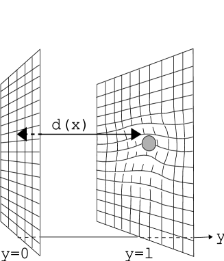
Figure 2: In the two brane system, the radion is defined as a distance between two branes. It could depend on the position because the brane could have bending. Hence, for observers on the brane, it appears as a scalar field.

7.1 Scalar-Tensor Theory Emerges

We consider the two-brane system depicted in Fig.2. Without matter on the branes, we have the relation $g^{\ominus\hbox{-}\rm brane}_{\mu\nu}=e^{-2d/\ell}g^{\oplus\hbox{-}\rm brane}\equiv\Omega^{2}g^{\oplus\hbox{-}\rm brane}$ where $d$ is the distance between the two branes. Although $\Omega$ is constant for vacuum branes, it becomes the function of the 4-dimensional coordinates if we put the matter on the brane.

Adding the energy momentum tensor to each of the two branes, and allowing deviations from the pure AdS₅ bulk, the effective (non-local) Einstein equations on the branes at low energies take the formsodKS2 ,

$$G^{\mu}{}_{\nu}(h) = {\kappa^{2}\over\ell}\overset{\oplus}{T}{}^{\mu}{}_{\nu}-{2\over\ell}\chi^{\mu}{}_{\nu}\,,$$ (87)

$$G^{\mu}{}_{\nu}(f) = -{\kappa^{2}\over\ell}\overset{\ominus}{T}{}^{\mu}{}_{\nu}-{2\over\ell}{\chi^{\mu}{}_{\nu}\over\Omega^{4}}\ .$$ (88)

where $h_{\mu\nu}=g^{\oplus\hbox{-}{\rm brane}}_{\mu\nu}$, $f_{\mu\nu}=g^{\ominus\hbox{-}{\rm brane}}_{\mu\nu}=\Omega^{2}h_{\mu\nu}$ and the terms proportional to $\chi_{\mu\nu}$ are 5-dimensional Weyl tensor contributions which describe the non-local 5-dimensional effect. Although Eqs. (87) and (88) are non-local individually, with undetermined $\chi_{\mu\nu}$, one can combine both equations to reduce them to local equations for each brane. Since $\chi_{\mu\nu}$ appears only algebraically, one can easily eliminate $\chi_{\mu\nu}$ from Eqs. (87) and (88). Defining a new field $\Psi=1-\Omega^{2}$, we find

$$G^{\mu}{}_{\nu}(h) = {\kappa^{2}\over\ell\Psi}\overset{\oplus}{T}{}^{\mu}{}_{\nu}+{\kappa^{2}(1-\Psi)^{2}\over\ell\Psi}\overset{\ominus}{T}{}^{\mu}{}_{\nu}$$ (89)

$$+{1\over\Psi}\left(\Psi^{|\mu}{}_{|\nu}-\delta^{\mu}_{\nu}\Psi^{|\alpha}{}_{|\alpha}\right)$$

$$+{3\over 2\Psi(1-\Psi)}\left(\Psi^{|\mu}\Psi_{|\nu}-{1\over 2}\delta^{\mu}_{\nu}\Psi^{|\alpha}\Psi_{|\alpha}\right),$$

$$\Box\Psi = {\kappa^{2}\over 3\ell}(1-\Psi)\left\{\overset{\oplus}{T}+(1-\Psi)\overset{\ominus}{T}\right\}-{1\over 2(1-\Psi)}\Psi^{|\mu}\Psi_{|\mu}\ ,$$ (90)

where $|$ denotes the covariant derivative with respect to the metric $h_{\mu\nu}$. Since $\Omega$ (or equivalently $\Psi$) contains the information of the distance between the two branes, we call $\Omega$ (or $\Psi$) the radion.

We can also determine $\chi^{\mu}{}_{\nu}$ by eliminating $G^{\mu}{}_{\nu}$ from Eqs. (87) and (88). Then,

$$\chi^{\mu}{}_{\nu} = -{\kappa^{2}(1-\Psi)\over 2\Psi}\left(\overset{\oplus}{T}{}^{\mu}{}_{\nu}+(1-\Psi)\overset{\ominus}{T}{}^{\mu}{}_{\nu}\right)$$ (91)

$$-{\ell\over 2\Psi}\left[\left(\Psi^{|\mu}{}_{|\nu}-\delta^{\mu}_{\nu}\Psi^{|\alpha}{}_{|\alpha}\right)\right.$$

$$\left.+{3\over 2(1-\Psi)}\left(\Psi^{|\mu}\Psi_{|\nu}-{1\over 2}\delta^{\mu}_{\nu}\Psi^{|\alpha}\Psi_{|\alpha}\right)\right]\ .$$

Note that the index of $\overset{\ominus}{T}{}^{\mu}{}_{\nu}$ is to be raised or lowered by the induced metric on the $\ominus$-brane, $f_{\mu\nu}$.

The effective action for the $\oplus$-brane which gives Eqs. (89) and (90) is

$$S_{\oplus} = {\ell\over 2\kappa^{2}}\int d^{4}x\sqrt{-h}\left[\Psi R-{3\over 2(1-\Psi)}\Psi^{|\alpha}\Psi_{|\alpha}\right]$$ (92)

$$\!\!\!\!\!\!\!\!\!\!+\int d^{4}x\sqrt{-h}{\cal L}^{\oplus}+\int d^{4}x\sqrt{-h}\left(1-\Psi\right)^{2}{\cal L}^{\ominus}\ .$$

The above action can be used to make cosmological predictions sodKoyama:2003be . It should be stressed that the radion has the conformal coupling. In fact, using the transformation $\Psi=1-\psi^{2}$, we obtain

$$S_{\oplus}={6\ell\over\kappa^{2}}\int d^{4}x\sqrt{-h}\left[\frac{1}{12}R-\frac{1}{12}\psi^{2}R-\frac{1}{2}\psi^{|\alpha}\psi_{|\alpha}\right]+\cdots\ .$$ (93)

This is nothing but Einstein theory with a conformally coupled scalar field $\psi$.

7.2 AdS/CFT in two-brane system?

In the two-brane case, it is difficult to proceed to the next order calculations. Hence, we need to invent a new method sodKanno:2003vf . For this purpose, we shall start with the effective Einstein equation obtained by Shromizu, Maeda, and Sasaki sodShiMaSa

$$G_{\mu\nu}=T_{\mu\nu}+\pi_{\mu\nu}-E_{\mu\nu}$$ (94)

where $\pi_{\mu\nu}$ is the quadratic of energy momentum tensor $T_{\mu\nu}$ and $E_{\mu\nu}$ represents the effect of the bulk geometry. Here we have set $8\pi G=1$. This geometrical projection approach can not give a concrete prediction, because we do not know $E_{\mu\nu}$ without solving the equations of motion in the bulk. Fortunately, in the case of the homogeneous cosmology, the property $E^{\mu}{}_{\mu}=0$ determines the dynamics as

$$H^{2}={1\over 3}\rho+\rho^{2}+{{\cal C}\over a^{4}}\ .$$ (95)

This reflects the interplay between the bulk and the brane dynamics on the brane.

What we want to seek is an effective theory which contains the information of the bulk as finite number of constant parameters like ${\cal C}$ in the homogeneous universe. When we succeed in obtaining it, the cosmological perturbation theory can be constructed in a usual way. Although the concrete prediction can not be made, qualitative understanding of the evolution of the cosmological fluctuations can be obtained. This must be useful to make observational predictions.

In the two-brane system, the mass spectrum is known from the linear analysis sodGT . At low energy, the propagator for the KK mode with the mass $m$ can be expanded as

$${-1\over\Box-m^{2}}={1\over m^{2}}\left[1+{\Box\over m^{2}}+{\Box^{2}\over m^{4}}+\cdots\right]\ .$$ (96)

However, massless modes can not be expanded in this way, hence we must take into account all of the massless modes to construct braneworld effective action. It seems legitimate to assume this consideration is valid even in the non-linear regime. Thus, at low energy, the action can be expanded by the local terms with increasing orders of derivatives of the metric $g_{\mu\nu}$ and the radion $\Psi$ sodKS2 .

Let us illustrate our method using the following action truncated at the second order derivatives:

$$S_{\rm eff}={1\over 2}\int d^{4}x\sqrt{-g}\left[\Psi R-2\Lambda(\Psi)-{\omega(\Psi)\over\Psi}\nabla^{\mu}\Psi\nabla_{\mu}\Psi\right]\ ,$$ (97)

which is nothing but the scalar-tensor theory with coupling function $\omega(\Psi)$ and the potential function $\Lambda(\Psi)$. Note that this is the most general local action which contains up to the second order derivatives and has the general coordinate invariance. It should be stressed that the scalar-tensor theory is, in general, not related to the braneworld. However, we know a special type of scalar-tensor theory corresponds to the low energy braneworld sodKS2 ; sodShiKo ; sodSK ; sodwiseman ; sodchiba ; sodKobayashi:2002pw . Here, we will present a simple derivation of this known fact.

For the vacuum brane, we can put $T_{\mu\nu}+\pi_{\mu\nu}=-\lambda g_{\mu\nu}$. Hence, the geometrical effective equation reduces to

$$G_{\mu\nu}=-E_{\mu\nu}-\lambda g_{\mu\nu}\ .$$ (98)

First, we must find $E_{\mu\nu}$. The above action (97) gives the equations of motion for the metric as

$$G_{\mu\nu} = -{\Lambda\over\Psi}g_{\mu\nu}+{1\over\Psi}\left(\nabla_{\mu}\nabla_{\nu}\Psi-g_{\mu\nu}\Box\Psi\right)$$ (99)

$$+{\omega\over\Psi^{2}}\left(\nabla_{\mu}\Psi\nabla_{\nu}\Psi-{1\over 2}g_{\mu\nu}\nabla^{\alpha}\Psi\nabla_{\alpha}\Psi\right)\ .$$

The right hand side of this Eq. (99) should be identified with $-E_{\mu\nu}-\lambda g_{\mu\nu}$. Hence, the condition $E^{\mu}{}_{\mu}=0$ becomes

$$\Box\Psi=-{\omega\over 3\Psi}\nabla^{\mu}\Psi\nabla_{\mu}\Psi-{4\over 3}\left(\Lambda-\lambda\Psi\right)\ .$$ (100)

This is the equation for the radion $\Psi$. However, we also have the equation for $\Psi$ from the action (97) as

$$\Box\Psi=\left({1\over 2\Psi}-{\omega^{\prime}\over 2\omega}\right)\nabla^{\alpha}\Psi\nabla_{\alpha}\Psi-{\Psi\over 2\omega}R+{\Psi\over\omega}\Lambda^{\prime}\ ,$$ (101)

where the prime denotes the derivative with respect to $\Psi$. In order for these two Eqs. (100) and (101) to be compatible, $\Lambda$ and $\omega$ must satisfy

$$-{\omega\over 3\Psi}={1\over 2\Psi}-{\omega^{\prime}\over 2\omega}\ ,$$ (102)

$${4\over 3}\left(\Lambda-\lambda\Psi\right)={\Psi\over\omega}\left(2\lambda-\Lambda^{\prime}\right)\ ,$$ (103)

where we used $R=4\lambda$ which comes from the trace part of Eq. (98). Eqs. (102) and (103) can be integrated as

$$\Lambda(\Psi)=\lambda+\lambda\gamma\left(1-\Psi\right)^{2}\ ,\quad\omega(\Psi)={3\over 2}{\Psi\over 1-\Psi}\ ,$$ (104)

where the constant of integration $\gamma$ represents the ratio of the cosmological constant on the negative tension brane to that on the positive tension brane. Here, one of constants of integration is absorbed by rescaling of $\Psi$. In doing so, we have assumed the constant of integration is positive. We can also describe the negative tension brane if we take the negative signature.

Thus, we get the effective action

$$S_{\rm eff}=\int d^{4}x\sqrt{-g}\left[{1\over 2}\Psi R-{3\over 4(1-\Psi)}\nabla^{\mu}\Psi\nabla_{\mu}\Psi-\lambda-\lambda\gamma(1-\Psi)^{2}\right]\ .$$ (105)

Surprisingly, this completely agrees with the previous result (92). Our simple symmetry principle $E^{\mu}{}_{\mu}=0$ has determined the action completely.

As we have shown in sodKSS , if $\gamma<-1$ there exists a static deSitter two-brane solution which turns out to be unstable. In particular, two inflating branes can collide at $\Psi=0$. This process is completely smooth for the observer on the brane. This fact led us to the born-again scenario sodKSS ; sodKanno:2005vq . The similar process occurs also in the ekpyrotic (cyclic) model sodturok where the moduli approximation is used. It can be shown that the moduli approximation is nothing but the lowest order truncation of the low energy gradient expansion method developed by us sodKanno:2004yb ; sodKanno:2005zr ; sodBrax:2002nt ; sodMcFadden:2004ni . Hence, it is of great interest to see the leading order corrections due to KK modes to this process.

Let us now apply the conformal symmetry method explained above to the higher order case. First, we need to write down the most generic action containing up to fourth order derivatives. Then, we impose the symmetry to determine unknown functionals. The action reads

$$S_{\rm eff}\!\! = \!\!{1\over 2}\int d^{4}x\sqrt{-g}\left[\Psi R-2\Lambda(\Psi)-{\omega(\Psi)\over\Psi}\nabla^{\mu}\Psi\nabla_{\mu}\Psi\right]$$ (106)

$$\!\!+\int d^{4}x\sqrt{-g}\left[A(\Psi)\left(\nabla^{\mu}\Psi\nabla_{\mu}\Psi\right)^{2}+B(\Psi)\left(\Box\Psi\right)^{2}\right.$$

$$\left.\quad\qquad+C(\Psi)\nabla^{\mu}\Psi\nabla_{\mu}\Psi\Box\Psi+D(\Psi)R~{}\Box\Psi\right.$$

$$\left.\quad\qquad+E(\Psi)R\nabla^{\mu}\Psi\nabla_{\mu}\Psi+F(\Psi)R^{\mu\nu}\nabla_{\mu}\Psi\nabla_{\nu}\Psi\right.$$

$$\left.\quad\qquad+G(\Psi)R^{2}+H(\Psi)R^{\mu\nu}R_{\mu\nu}\right.$$

$$\left.\quad\qquad+I(\Psi)R^{\mu\nu\lambda\rho}R_{\mu\nu\lambda\rho}+\cdots\right]\ ,$$

where $A,B,\cdots$ denote arbitrary functionals of the radion.

Now we impose the conformal symmetry on the fourth order derivative terms in the action (106) as we did in the previous example. Starting from the action (106), one can read off the equation for the metric from which $E_{\mu\nu}$ can be identified. The compatibility between the equations of motion for $\Psi$ and the equation $E^{\mu}{}_{\mu}=0$ constrains the coefficient functionals in the action (106). Surprisingly, every coefficient functionals are determined up to constants.

Thus, we find the 4-dimensional effective action with KK corrections as

$$S_{\rm eff} = \int d^{4}x\sqrt{-g}\left[{1\over 2}\Psi R-{3\over 4(1-\Psi)}\nabla^{\mu}\Psi\nabla_{\mu}\Psi\right.$$ (107)

$$\left.\quad-\lambda-\lambda\gamma(1-\Psi)^{2}\right]$$

$$+\ell^{2}\int d^{4}x\sqrt{-g}\left[{1\over 4(1-\Psi)^{4}}\left(\nabla^{\mu}\Psi\nabla_{\mu}\Psi\right)^{2}\right.$$

$$\left.+{1\over(1-\Psi)^{2}}\left(\Box\Psi\right)^{2}+{1\over(1-\Psi)^{3}}\nabla^{\mu}\Psi\nabla_{\mu}\Psi\Box\Psi\right.$$

$$\left.+{2\over 3(1-\Psi)}R\Box\Psi+{1\over 3(1-\Psi)^{2}}R\nabla^{\mu}\Psi\nabla_{\mu}\Psi\right.$$

$$\left.+jR^{2}+kR^{\mu\nu}R_{\mu\nu}\right]\ ,$$

where constants $j$ and $k$ can be interpreted as the variety of the effects of the bulk gravitational waves. These constants have the same origin as the previous parameters $\alpha$ and $\beta$. It should be noted that this action becomes non-local after integrating out the radion field. This fits the fact that KK effects are non-local usually. In principle, we can continue this calculation to any order of derivatives.

8 The Answers

We have developed the low energy gradient expansion scheme to give insights into the physics of the braneworld such as the black hole physics and the cosmology. In particular, we have concentrated on the specific questions in this lecture. Here, we summarize our answers obtained by the gradient expansion method. Our understanding of RS braneworlds would be also useful for other brane models.

8.1 Single-brane model

Is the Einstein theory recovered even in the non-linear regime?

We have obtained the effective theory at the lowest order as

$$\overset{(4)}{G}{}^{\mu}{}_{\nu}={\kappa^{2}\over\ell}T^{\mu}{}_{\nu}-{2\over\ell}\chi^{\mu}{}_{\nu}\ .$$ (108)

Here we have the correction $\chi_{\mu\nu}$ which can be interpreted as the dark radiation in the cosmological situation.

On the other hand, in the linearized gravity, the conventional Einstein theory is recovered at low energy. This is because the out-going boundary condition is imposed. In other words, the asymptotic AdS boundary condition is imposed. In the nonlinear case, this corresponds to the requirement that the dark radiation term $\chi_{\mu\nu}$ must be zero. For this boundary condition, the conventional Einstein theory is recovered. Hence, the standard Friedmann equation holds.

In this sense, the answer is yes.

How does the AdS/CFT come into the braneworld?

The CFT emerges as the constant of integration which satisfies the trace anomaly relation

$$\tau^{\mu}{}_{\mu}=-{1\over 8}\left(R^{\alpha}{}_{\beta}R^{\beta}{}_{\alpha}-{1\over 3}R^{2}\right)-\beta\Box R\ .$$ (109)

This constant can not be determined a priori. Here, the AdS/CFT correspondence could come into the braneworld. Namely, if we identify some CFT with $\tau_{\mu\nu}$, then we can determine the boundary condition.

How are the AdS/CFT and geometrical approach related?

The key quantity in the geometric approach is obtained as

$$\overset{(2)}{E}{}^{\mu}{}_{\nu}=\ell^{2}\left[P^{\mu}{}_{\nu}+2\tau^{\mu}{}_{\nu}+2\alpha{\cal S}^{\mu}{}_{\nu}+{2\over 3}\beta{\cal K}^{\mu}{}_{\nu}\right]\ .$$ (110)

The above expression contains $\tau_{\mu\nu}$ which can be interpreted as the CFT matter. Hence, once we know $E_{\mu\nu}$, no enigma remains. In particular, $P_{\mu\nu}\approx\pi_{\mu\nu}$ is independent of the $\tau_{\mu\nu}$. In odd dimensions, there exists no trace anomaly, but $P_{\mu\nu}$ exists. In 4-dimensions, $\pi^{\mu}{}_{\mu}$ accidentally coincides with the trace anomaly in CFT.

It is interesting to note that the high energy and the Weyl term corrections found in the geometrical approach merge into the CFT matter correction found in the AdS/CFT approach.

8.2 Two-brane model

How is the geometrical approach consistent with the Brans-Dicke picture?

In the geometrical approach, no radion seems to appear. On the other hand, the linear theory predicts the radion as the crucial quantity. The resolution can be attained by obtaining $E_{\mu\nu}$ ($\chi_{\mu\nu}$ in our notation). The resultant expression

$$\chi^{\mu}{}_{\nu} = -{\kappa^{2}(1-\Psi)\over 2\Psi}\left(\overset{\oplus}{T}{}^{\mu}{}_{\nu}+(1-\Psi)\overset{\ominus}{T}{}^{\mu}{}_{\nu}\right)$$

$$-{\ell\over 2\Psi}\left[\left(\Psi^{|\mu}{}_{|\nu}-\delta^{\mu}_{\nu}\Psi^{|\alpha}{}_{|\alpha}\right)\right.$$

$$\left.+{3\over 2(1-\Psi)}\left(\Psi^{|\mu}\Psi_{|\nu}-{1\over 2}\delta^{\mu}_{\nu}\Psi^{|\alpha}\Psi_{|\alpha}\right)\right]$$

contains the radion in an intriguing way. The dark radiation consists of the radion and the matter.

We have shown that the radion transforms the Einstein theory with Weyl correction into the conformally coupled scalar-tensor theory where the radion plays the role of the scalar field. Thus, it turned out that the radion is hidden by the projected Weyl tensor $E_{\mu\nu}$ in the geometrical approach.

What replaces the AdS/CFT correspondence in the two-brane model?

In the case of the single-brane model, the out-going boundary condition at the Cauchy horizon is assumed. This conforms to AdS/CFT correspondence. Indeed, the continuum KK-spectrum are projected on the brane as CFT matter.

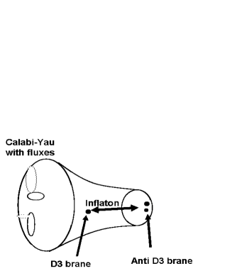
Figure 3: The warped throat is attached to Calabi-Yau manifold. Anti-D3-branes are stacked at the tip of the warped throat. A D3-brane can move in the throat and the radion, i.e. the distance between the D3-brane and anti-D3-branes, plays a role of the inflaton.

On the other hand, the boundary condition in the two-brane system allows only the discrete KK-spectrum. Hence, we can not expect CFT matter on the brane. Instead, the radion controls the bulk/brane correspondence in two-brane model. In fact, the higher derivative terms of the radion mimics the effect of the bulk geometry (KK-effect) as we have shown explicitly. Hence, the conventional AdS/CFT correspondence does not exist. Instead, there exists the AdS/CFT correspondence realized by the conformally coupled radion. The conformal coupling can be regarded as a reflection of the symmetry of the bulk geometry.

Here, I would like to mention D-brane inflation models proposed in sodKachru:2003sx . There, the inflaton is identified as the radion which is the distance between a D3-brane and anti-D3-branes as is shown in Fig.3. Naively, it seems possible to realize a slow roll inflation due to the warped geometry. However, our result of two-brane system suggests the existence of the conformal coupling of the radion, which ruins the slow role inflation of the model. In fact, the curvature coupling gives a large mass of the inflaton which causes the notorious eta problem. Hence, a fine tuning is unavoidable.

9 AdS/CFT in Dilatonic braneworld

In the previous sections, we have considered RS braneworlds. If we take into account bulk fields, the pure AdS bulk would not be expected. Hence, it is interesting to see the role of AdS/CFT correspondence in those cases. In this section, we will consider a bulk scalar field and call this kind of models dilatonic braneworlds sodMaeda:2000wr .

In addition to the above theoretical interest, there is an phenomenological intererest in dilatonic braneworlds. Let us see how the inflationary universe can be realized in the braneworld. The formula for the effective cosmological constant in the braneworld reads

$$\Lambda_{\rm eff}={\kappa^{4}\sigma^{2}\over 12}-{3\over\ell^{2}}\ ,$$ (111)

where $\sigma$ and $\ell$ are the tension of the brane and the curvature scale in the bulk which is determined by the bulk vacuum energy, respectively. For $\kappa^{2}\sigma=6/\ell$, we have Minkowski spacetime. In order to obtain the inflationary universe, we need the positive effective cosmological constant. In the braneworld model, there are two possibilities. One is to increase the brane tension and the other is to increase $\ell$. The brane tension can be controlled by the scalar field on the brane. The bulk curvature scale $\ell$ can be controlled by the bulk scalar field. The former case is a natural extension of the 4-dimensional inflationary scenario. The latter possibility is a novel one peculiar to the brane model. Recall that, in the superstring theory, scalar fields are ubiquitous. Indeed, the dilaton and moduli exists in the bulk generically, because they arise as the modes associated with the closed string. Moreover, when the supersymmetry is spontaneously broken, they may have the non-trivial potential. Hence, it is natural to consider the inflationary scenario driven by these fields sodKobayashi:2000yh ; sodHimemoto:2000nd . Therefore, dilatonic braneworlds are phenomenologically interesting. In this section, we would like to discuss this dilatonic braneworld from the point of view of the AdS/CFT correspondence.

9.1 Dilatonic Braneworld

We consider a $S_{1}/Z_{2}$ orbifold spacetime with the two branes as the fixed points. In this first Randall-Sundrum (RS1) model, the two flat 3-branes are embedded in AdS₅ and the brane tensions given by $\overset{\oplus}{\sigma}=6/(\kappa^{2}\ell)$ and $\overset{\ominus}{\sigma}=-6/(\kappa^{2}\ell)$. Our system is described by the action

$$S = {1\over 2\kappa^{2}}\int d^{5}x\sqrt{-g}~{}{\cal R}-\int d^{5}x\sqrt{-g}\left[~{}{1\over 2}g^{AB}\partial_{A}\varphi\partial_{B}\varphi+U(\varphi)~{}\right]$$ (112)

$$-\sum_{i=\oplus,\ominus}\overset{i}{\sigma}\int d^{4}x\sqrt{-g^{i\mathrm{\hbox{-}brane}}}+\sum_{i=\oplus,\ominus}\int d^{4}x\sqrt{-g^{i\mathrm{\hbox{-}brane}}}\,{\cal L}_{\rm matter}^{i}\ ,$$

where $g^{i\mathrm{\hbox{-}brane}}_{\mu\nu}$ and $\overset{i}{\sigma}$ are the induced metric and the brane tension on the $i$-brane, respectively. We assume the potential $U(\varphi)$ for the bulk scalar field takes the form $U(\varphi)=-\frac{6}{\kappa^{2}\ell^{2}}+V(\varphi)\ ,$ where the first term is regarded as a 5-dimensional cosmological constant and the second term is an arbitrary potential function. The brane tension $\sigma$ is tuned so that the effective cosmological constant on the brane vanishes. The above setup realizes a flat braneworld after inflation ends and the field $\varphi$ reaches the minimum of its potential.

Inflation in the braneworld can be driven by a scalar field either on the brane or in the bulk. We derive the effective equations of motion which are useful for both models. Here, we begin with the single-brane system. Since we know the effective 4-dimensional equations hold irrespective of the existence of other branes sodKS4 , the analysis of the single-brane system is sufficient to derive the effective action for the two-brane system as we see in the next subsection.

We again adopt the Gaussian normal coordinate system to describe the geometry of the brane model; $ds^{2}=dy^{2}+g_{\mu\nu}(y,x^{\mu})dx^{\mu}dx^{\nu}\ ,$ where the brane is assumed to be located at $y=0$. Let us decompose the extrinsic curvature into the traceless part $\Sigma_{\mu\nu}$ and the trace part $K$ as $K_{\mu\nu}=-\frac{1}{2}g_{\mu\nu,y}=\Sigma_{\mu\nu}+{1\over 4}g_{\mu\nu}K\ .$ Then, we can obtain the basic equations off the brane using these variables. First, the Hamiltonian constraint equation leads to

$${3\over 4}K^{2}-\Sigma^{\alpha}{}_{\beta}\Sigma^{\beta}{}_{\alpha} = \overset{(4)}{R}-\kappa^{2}\nabla^{\alpha}\varphi\nabla_{\alpha}\varphi+\kappa^{2}(\partial_{y}\varphi)^{2}-2\kappa^{2}U(\varphi)\ ,$$ (113)

where $\overset{(4)}{R}$ is the curvature on the brane and $\nabla_{\mu}$ denotes the covariant derivative with respect to the metric $g_{\mu\nu}$. Momentum constraint equation becomes

$$\nabla_{\lambda}\Sigma_{\mu}{}^{\lambda}-{3\over 4}\nabla_{\mu}K=-\kappa^{2}\partial_{y}\varphi\partial_{\mu}\varphi\ .$$ (114)

Evolution equation in the direction of $y$ is given by

$$\Sigma^{\mu}{}_{\nu,y}-K\Sigma^{\mu}{}_{\nu}=-\left[\overset{(4)}{R}{}_{\mu\nu}-\kappa^{2}\nabla^{\mu}\varphi\nabla_{\nu}\varphi\right]_{\rm traceless}\ .$$ (115)

Finally, the equation of motion for the scalar field reads

$$\partial^{2}_{y}\varphi-K\partial_{y}\varphi+\nabla^{\alpha}\nabla_{\alpha}\varphi-U^{\prime}(\varphi)=0\ ,$$ (116)

where the prime denotes derivative with respect to the scalar field $\varphi$.

As we have the singular source at the brane position, we must consider the junction conditions. Assuming a $Z_{2}$ symmetry of spacetime, we obtain the junction conditions for the metric and the scalar field

$$\left[\Sigma^{\mu}{}_{\nu}-{3\over 4}\delta^{\mu}_{\nu}K\right]\Bigg{|}_{y=0} = -{\kappa^{2}\over 2}\sigma\delta^{\mu}_{\nu}+\frac{\kappa^{2}}{2}T^{\mu}{}_{\nu}\ ,$$ (117)

$$\Bigl{[}\partial_{y}\varphi\Bigr{]}\bigg{|}_{y=0} = 0\ ,$$ (118)

where $T^{\mu}{}_{\nu}$ is the energy-momentum tensor for the matter fields on the brane.

9.2 AdS/Radion correspondence

We assume the inflation occurs at low energy in the sense that the additional energy due to the bulk scalar field is small, $\kappa^{2}\ell^{2}V(\varphi)\ll 1$, and the curvature on the brane $R$ is also small, $R\ell^{2}\ll 1$. It should be stressed that the low energy does not necessarily implies weak gravity on the brane. Under these circumstances, we can use a gradient expansion scheme to solve the bulk equations of motion.

At zeroth order, we ignore matters on the brane. Then, from the junction condition (117), we have

$$\left[\overset{(0)}{\Sigma}{}^{\mu}{}_{\nu}-{3\over 4}\delta^{\mu}_{\nu}\overset{(0)}{K}\right]\Bigg{|}_{y=0} = -{\kappa^{2}\over 2}\sigma\delta^{\mu}_{\nu}\ .$$ (119)

As the right hand side of (119) contains no traceless part, we get $\overset{(0)}{\Sigma}{}^{\mu}{}_{\nu}=0\ .$ We also take the potential for the bulk scalar field $U(\varphi)$ to be $-6/(\kappa^{2}\ell^{2})$. We discard the terms with 4-dimensional derivatives since one can neglect the long wavelength variation in the direction of $x^{\mu}$ at low energies. Thus, the equations to be solved are given by

$${3\over 4}\overset{(0)}{K}{}^{2}=\kappa^{2}(\partial_{y}\overset{(0)}{\varphi})^{2}+{12\over\ell^{2}}\ ,$$ (120)

$$\partial^{2}_{y}\overset{(0)}{\varphi}-\overset{(0)}{K}\partial_{y}\overset{(0)}{\varphi}=0\ .$$ (121)

The junction condition (118) at this order $\Bigl{[}\partial_{y}\overset{(0)}{\varphi}\Bigr{]}\bigg{|}_{y=0}=0$ tells us that the solution of Eq.(121) must be $\overset{(0)}{\varphi}=\eta~{}(x^{\mu})\ ,$ where $\eta(x^{\mu})$ is an arbitrary constant of integration. Now, the solution of Eq.(121) yields $\overset{(0)}{K}={4/\ell}\ .$ Other Eqs. (114) and (115) are trivially satisfied at zeroth order. Using the definition $\overset{(0)}{K}{}_{\mu\nu}=-\overset{(0)}{g}_{\mu\nu,y}/2$, we have the lowest order metric

$$\overset{(0)}{g}{}_{\mu\nu}(y,x^{\mu})=b^{2}(y)~{}h_{\mu\nu}(x^{\mu}),\qquad b(y)\equiv e^{-y/\ell}\ ,$$ (122)

where the induced metric on the brane, $h_{\mu\nu}\equiv g_{\mu\nu}(y=0,x^{\mu})$, arises as a constant of integration. The junction condition for the induced metric (119) merely implies well known relation $\kappa^{2}\sigma=6/\ell$ and that for the scalar field (118) is trivially satisfied. At this leading order analysis, we can not determine the constants of integration $h_{\mu\nu}(x^{\mu})$ and $\eta(x^{\mu})$ which are constant as far as the short length scale $\ell$ variations are concerned, but are allowed to vary over the long wavelength scale. These constants should be constrained by the next order analysis.

Now, we take into account the effect of both the bulk scalar field and the matter on the brane perturbatively. Our iteration scheme is to write the metric $g_{\mu\nu}$ and the scalar field $\varphi$ as a sum of local tensors built out of the induced metric and the induced scalar field on the brane, in the order of expansion parameters, that is, $O((R\ell^{2})^{n})$ and $O(\kappa^{2}\ell^{2}V(\varphi))^{n}$, $n=0,1,2,\cdots$ sodKS4 . Then, we expand the metric and the scalar field as

$$g_{\mu\nu}(y,x^{\mu})=b^{2}(y)\left[h_{\mu\nu}(x^{\mu})+\overset{(1)}{g}_{\mu\nu}(y,x^{\mu})+\overset{(2)}{g}_{\mu\nu}(y,x^{\mu})+\cdots\right]\ ,$$

$$\varphi(y,x^{\mu})=\eta(x^{\mu})+\overset{(1)}{\varphi}(y,x^{\mu})+\overset{(2)}{\varphi}(y,x^{\mu})+\cdots\ .$$ (123)

Here, we put the boundary conditions $\overset{(i)}{g}_{\mu\nu}(y=0,x^{\mu})=0\ ,\overset{(i)}{\varphi}(y=0,x^{\mu})=0\ ,\quad i=1,2,3,...$ so that we can interpret $h_{\mu\nu}$ and $\eta$ as induced quantities. Extrinsic curvatures can be also expanded as

$$K=\frac{4}{\ell}+\overset{(1)}{K}+\overset{(2)}{K}+\cdots\ ,\qquad\Sigma^{\mu}_{\ \nu}=\overset{(1)}{\Sigma}{}^{\mu}_{\ \nu}+\overset{(2)}{\Sigma}{}^{\mu}_{\ \nu}+\cdots\ .$$ (124)

Using the formula such as $\overset{(4)}{R}(\overset{(0)}{g}_{\mu\nu})=R(h_{\mu\nu})/b^{2}$, we obtain the solution

$$\overset{(1)}{K}=\frac{\ell}{6b^{2}}\left(R(h)-\kappa^{2}\eta^{|\alpha}\eta_{|\alpha}\right)-\frac{\ell}{3}\kappa^{2}V(\eta)\ ,$$ (125)

where $R(h)$ is the scalar curvature of $h_{\mu\nu}$ and $|$ denotes the covariant derivative with respect to $h_{\mu\nu}$. Substituting the results at zeroth order solutions into Eq. (115), we obtain

$$\overset{(1)}{\Sigma}{}^{\mu}{}_{\nu}=\frac{\ell}{2b^{2}}\left[R^{\mu}{}_{\nu}(h)-\kappa^{2}\eta^{|\mu}\eta_{|\nu}\right]_{\rm traceless}+\frac{\chi^{\mu}{}_{\nu}}{b^{4}}\ ,$$ (126)

where $R^{\mu}{}_{\nu}(h)$ denotes the Ricci tensor of $h_{\mu\nu}$ and $\chi^{\mu}{}_{\nu}$ is a constant of integration which satisfies the constraint $\chi^{\mu}{}_{\mu}=0$. Hereafter, we omit the argument of the curvature for simplicity. Integrating the scalar field equation (116) at first order, we have

$$\partial_{y}\overset{(1)}{\varphi} = \frac{\ell}{2b^{2}}\Box\eta-\frac{\ell}{4}V^{\prime}(\eta)+\frac{C}{b^{4}}\ ,$$ (127)

where $C$ is also a constant of integration. At first order in this iteration scheme, we get two kinds of constants of integration, $\chi^{\mu}{}_{\nu}$ and $C$.

Given the matter fields $T_{\mu\nu}$ on the brane, the junction condition (117) becomes

$$\left[\overset{(1)}{\Sigma}{}^{\mu}{}_{\nu}-\frac{3}{4}\delta^{\mu}_{\nu}\overset{(1)}{K}\right]\Bigg{|}_{y=0}=\frac{\kappa^{2}}{2}T^{\mu}{}_{\nu}\ .$$ (128)

At this order, the junction condition (118) yields

$$\biggl{[}\partial_{y}\overset{(1)}{\varphi}\biggr{]}\Bigg{|}_{y=0}=0\ .$$ (129)

These junction conditions give the effective equations of motion on the brane.

Now, we are in a position to discuss the effective equations of motion for the dilatonic two-brane models. The point is the fact that the equations of motion on each brane take the same form if we use the induced metric on each brane sodKS4 . The effective Einstein equations on each positive ($\oplus$) and negative ($\ominus$) tension brane at low-energies yield

$$G^{\mu}{}_{\nu}(h) = \kappa^{2}\left(\eta^{|\mu}\eta_{|\nu}-{1\over 2}\delta^{\mu}_{\nu}\eta^{|\alpha}\eta_{|\alpha}-{1\over 2}\delta^{\mu}_{\nu}V\right)-{2\over\ell}\chi^{\mu}{}_{\nu}+\frac{\kappa^{2}}{\ell}\overset{\oplus}{T}{}^{\mu}{}_{\nu}\ ,$$ (130)

$$G^{\mu}{}_{\nu}(f) = \kappa^{2}\left(\eta^{;\mu}\eta_{;\nu}-{1\over 2}\delta^{\mu}_{\nu}\eta^{;\alpha}\eta_{;\alpha}-{1\over 2}\delta^{\mu}_{\nu}V\right)-{2\over\ell}{\chi^{\mu}{}_{\nu}\over\Omega^{4}}-\frac{\kappa^{2}}{\ell}\overset{\ominus}{T}{}^{\mu}{}_{\nu}\ .$$ (131)

where $f_{\mu\nu}$ is the induced metric on the negative tension brane and ; denotes the covariant derivative with respect to $f_{\mu\nu}$. When we set the position of the positive tension brane at $y=0$, that of the negative tension brane $\bar{y}$ in general depends on $x^{\mu}$, i.e. $\bar{y}=\bar{y}(x^{\mu})$. Hence, the warp factor at the negative tension brane $\Omega(x^{\mu})\equiv b(\bar{y}(x))$ also depends on $x^{\mu}$. Because the metric always comes into equations with derivatives, the zeroth order relation is enough in this first order discussion. Hence, the metric on the positive tension brane is related to the metric on the negative tension brane as $f_{\mu\nu}=\Omega^{2}h_{\mu\nu}$.

Although Eqs. (130) and (131) are non-local individually, with undetermined $\chi^{\mu}{}_{\nu}$, one can combine both equations to reduce them to local equations for each brane. We can therefore easily eliminate $\chi^{\mu}{}_{\nu}$ from Eqs. (130) and (131), since $\chi^{\mu}{}_{\nu}$ appears only algebraically. Eliminating $\chi^{\mu}{}_{\nu}$ from both Eqs. (130) and (131), we obtain

$$G^{\mu}{}_{\nu} = \frac{\kappa^{2}}{\ell\Psi}\overset{\oplus}{T}{}^{\mu}{}_{\nu}+\frac{\kappa^{2}(1-\Psi)^{2}}{\ell\Psi}\overset{\ominus}{T}{}^{\mu}{}_{\nu}$$ (132)

$$+{1\over\Psi}\left[\Psi^{|\mu}{}_{|\nu}-\delta^{\mu}_{\nu}\Psi^{|\alpha}{}_{|\alpha}+{3\over 2}{1\over 1-\Psi}\left(\Psi^{|\mu}\Psi_{|\nu}-{1\over 2}\delta^{\mu}_{\nu}\Psi^{|\alpha}\Psi_{|\alpha}\right)\right]$$

$$+\kappa^{2}\left(\eta^{|\mu}\eta_{|\nu}-\frac{1}{2}\delta^{\mu}_{\nu}\eta^{|\alpha}\eta_{|\alpha}-\delta^{\mu}_{\nu}V_{\rm eff}\right)\ ,\quad V_{\rm eff}=\frac{2-\Psi}{2}V\ ,$$

where we defined a new field $\Psi=1-\Omega^{2}$ which we refer to by the name “radion”. The bulk scalar field induces the energy-momentum tensor of the conventional 4-dimensional scalar field with the effective potential which depends on the radion.

We can also determine the dark radiation $\chi^{\mu}{}_{\nu}$ by eliminating $G^{\mu}{}_{\nu}(h)$ from Eqs. (130) and (131),

$${2\over\ell}\chi^{\mu}{}_{\nu} = -{1\over\Psi}\left[\Psi^{|\mu}{}_{|\nu}-\delta^{\mu}_{\nu}\Psi^{|\alpha}{}_{|\alpha}+{3\over 2}{1\over 1-\Psi}\left(\Psi^{|\mu}\Psi_{|\nu}-{1\over 2}\delta^{\mu}_{\nu}\Psi^{|\alpha}\Psi_{|\alpha}\right)\right]$$ (133)

$$+{\kappa^{2}\over 2}(1-\Psi)\delta^{\mu}_{\nu}V-\frac{\kappa^{2}}{\ell}\frac{1-\Psi}{\Psi}\left[\overset{\oplus}{T}{}^{\mu}{}_{\nu}+\left(1-\Psi\right)\overset{\ominus}{T}{}^{\mu}{}_{\nu}\right]\ .$$

Due to the property $\chi^{\mu}{}_{\mu}=0$, we have

$$\Box\Psi=\frac{\kappa^{2}}{3\ell}(1-\Psi)\left[\overset{\oplus}{T}+(1-\Psi)\overset{\ominus}{T}\right]-{1\over 2(1-\Psi)}\Psi^{|\alpha}\Psi_{|\alpha}-{2\kappa^{2}\over 3}\Psi(1-\Psi)V\ .$$ (134)

Note that Eqs. (132) and (134) are derived from a scalar-tensor type theory coupled to the additional scalar field.

Similarly, the equations for the scalar field on branes become

$$\Box_{h}\eta-{V^{\prime}\over 2}+{2\over\ell}C=0\ ,$$ (135)

$$\Box_{f}\eta-{V^{\prime}\over 2}+{2\over\ell}{C\over\Omega^{4}}=0\ ,$$ (136)

where the subscripts refer to the induced metric on each brane. Notice that the scalar field takes the same value for both branes at this order. Eliminating the dark source $C$ from these Eqs. (135) and (136), we find the equation for the scalar field takes the form

$$\Box_{h}\eta-V^{\prime}_{\rm eff}=-\frac{\Psi^{|\mu}}{\Psi}\eta_{|\mu}\ .$$ (137)

Notice that the radion acts as a source for $\eta$. And we can also get the dark source as

$${2\over\ell}C=-{V^{\prime}\over 2}(1-\Psi)+{\Psi^{|\mu}\over\Psi}\eta_{|\mu}\ .$$ (138)

Now the effective action for the positive tension brane which gives Eqs. (132), (134) and (137) can be read off as

$$S = {\ell\over 2\kappa^{2}}\int d^{4}x\sqrt{-h}\left[\Psi R-\frac{3}{2(1-\Psi)}\Psi^{|\alpha}\Psi_{|\alpha}-\kappa^{2}\Psi\left(\eta^{|\alpha}\eta_{|\alpha}+2V_{\rm eff}(\eta,\Psi)\right)\right]$$ (139)

$$+\int d^{4}x\sqrt{-h}~{}\overset{\oplus}{\cal L}+\int d^{4}x\sqrt{-h}~{}(1-\Psi)^{2}\overset{\ominus}{\cal L}\ ,$$

where the last two terms represent actions for the matter on each brane. Thus, we found the radion field couples with the induced metric and the induced scalar field on the brane non-trivially. Surprisingly, at this order, the nonlocality of $\chi_{\mu\nu}$ and $C$ are eliminated by the radion. We see the radion has a conformal coupling. However, in the present case, the radion couples to the dilaton field which breaks a conformal invariance. Hence, this gives non-conformal holography.

As this is a closed system, we can analyze a primordial spectrum to predict the cosmic background fluctuation spectrum sodSoda:2005mu . Interestingly, $\chi^{\mu}_{\nu}$ and $C$ vanishes in the single brane limit, $\Psi\rightarrow 1$, as can be seen from (133) and (138). The dynamics is simply governed by Einstein theory with the single scalar field. Therefore, we can conclude that the bulk inflaton can drive inflation when the slow role conditions are satisfied.

9.3 AdS/CFT and KK corrections: Single-brane cases

It would be important to take into account the KK effects as corrections to the leading order result. It can be accomplished in the single-brane models. Using our approach, in the single brane limit, we can deduce the effective action with KK corrections as sodKS4 ; sodKanno:2003xy ( see also sodSoda:2002ky ; sodSoda:2004hq )

$$S = \frac{\ell}{2\kappa^{2}}\int d^{4}x\sqrt{-h}\left[\left(1+\frac{\ell^{2}}{12}\kappa^{2}V\right)R-\kappa^{2}\left(1+\frac{\ell^{2}}{12}\kappa^{2}V-\frac{\ell^{2}}{4}V^{\prime\prime}\right)\eta^{|\alpha}\eta_{|\alpha}-2\kappa^{2}V_{\rm eff}\right.$$ (140)

$$\left.\hskip 71.13188pt-\frac{\ell^{2}}{4}\left(R^{\alpha\beta}R_{\alpha\beta}-\frac{1}{3}R^{2}\right)\right]+\int d^{4}x\sqrt{-h}~{}{\cal L}_{\rm matter}+S_{\rm CFT}\ ,$$

where the last term comes from the energy-momentum tensor of CFT matter $\tau_{\mu\nu}$ and the effective potential at this order is defined by

$$V_{\rm eff}=\frac{1}{2}V+\frac{\ell^{2}\kappa^{2}}{48}V^{2}-\frac{\ell^{2}}{64}V^{\prime 2}\ .$$ (141)

It is interesting to note that the effective potential contains the terms which looks like F-terms in supersymmetric models.

Thus, even in the dilatonic braneworld, the AdS/CFT correspondence seems to play an important role in the single-brane case.

10 Conclusion

In this lecture, I have reviewed the gradient expansion method in the context of braneworlds. Using the formalism, I have tried to explain how the AdS/CFT correspondence is related to the braneworld models.

In the case of the RS single-brane model, we clarified when the conventional Einstein equations hold at low energy. Moreover, we revealed the relation between the geometrical and the AdS/CFT correspondence approach using the gradient expansion method. We have shown that the high energy and the Weyl term corrections found in the geometrical approach correspond to the CFT matter corrections found in the AdS/CFT approach.

In the case of the RS two-brane sysytem, we showed that the AdS/CFT correspondence plays an important role in the sense that the low energy effective field theory can be described by the conformally coupled scalar-tensor theory where the radion plays the role of the scalar field. We also presented the symmetry method to derive KK corrections in the two-brane system.

These effective theories for RS braneworlds can be used to make cosmological predictions. More importantly, it turned out that the gradient expansion method provides a unified view of RS braneworlds.

We have also considered the bulk scalar field with a nontrivial potential and derived the non-linear low energy effective action for the dilatonic two-brane model using the gradient expansion method. As a result, we have shown that the effective theory reduces to the scalar-tensor theory with the non-trivial coupling between the radion and the bulk scalar field. Since the radion has a conformal coupling, the conformal symmetry is relevant even for the dilatonic braneworlds. In this sense, the AdS/CFT correspondence is related to dilatonic braneworlds. However, the radion couples to the scalar field which is non-conformal. Hence, the conformal invariance is violated.

Our phenomenological motivation to consider dilatonic braneworlds was a possibility of the bulk inflaton. Concerning to this issue, taking into account the fact that $\chi_{\mu\nu}$ and $C$ becomes zero when two branes get separated infinitely, one can conclude that the bulk inflaton can drive the inflation on the brane as far as the slow roll conditions are satisfied. We also obtained KK corrections in the single brane limit which contain CFT corrections.

These results tell us that there exist profound relations between braneworlds and the AdS/CFT correspondence, although the correspondence is slightly deformed in the dilatonic cases.

In this lecture, we have considered only codimesion-one braneworlds. It is important to extend the analysis to higher codimension models sodCline:2003ak ; sodBurgess:2004dh ; sodVinet:2005dg ; sodBostock:2003cv ; sodKanno:2004nr ; sodCharmousis:2009uk ; sodPapantonopoulos:2007fk ; sodPapantonopoulos:2006uj ; sodKanno:2007wj ; sodChen:2008sn . It is intriguing to study a role of the AdS/CFT correspondence in these higher codimension braneworlds.

- (1) J. Polchinski, String Theory I and II (Cambridge Univ. Press, Cambridge, 1998).
- (2) P. Horava and E. Witten, Nucl. Phys. B 460, 506 (1996) [arXiv:hep-th/9510209].
- (3) P. Horava and E. Witten, Nucl. Phys. B 475, 94 (1996) [arXiv:hep-th/9603142].
- (4) A. Lukas, B. A. Ovrut, K. S. Stelle and D. Waldram, Phys. Rev. D 59, 086001 (1999) [arXiv:hep-th/9803235].
- (5) I. Antoniadis, N. Arkani-Hamed, S. Dimopoulos and G. R. Dvali, Phys. Lett. B 436, 257 (1998) [arXiv:hep-ph/9804398].
- (6) N. Arkani-Hamed, S. Dimopoulos and G. R. Dvali, Phys. Rev. D 59, 086004 (1999) [arXiv:hep-ph/9807344].
- (7) K. Akama, Lect. Notes Phys. 176, 267 (1982) [arXiv:hep-th/0001113].
- (8) V. A. Rubakov and M. E. Shaposhnikov, Phys. Lett. B 125 (1983) 136.
- (9) L. Randall and R. Sundrum, Phys. Rev. Lett. 83, 3370 (1999) [arXiv:hep-ph/9905221].
- (10) L. Randall and R. Sundrum, Phys. Rev. Lett. 83, 4690 (1999) [arXiv:hep-th/9906064].
- (11) S. Kanno and J. Soda, TSPU Vestnik 44N7, 15 (2004) [arXiv:hep-th/0407184].
- (12) K. Tomita, Prog. Theor. Phys. 54, 730 (1975).
- (13) D. S. Salopek and J. M. Stewart, Phys. Rev. D 47, 3235 (1993).
- (14) G. L. Comer, N. Deruelle, D. Langlois and J. Parry, Phys. Rev. D 49 (1994) 2759.
- (15) J. Soda, H. Ishihara and O. Iguchi, Prog. Theor. Phys. 94, 781 (1995) [arXiv:gr-qc/9509008].
- (16) P. Brax, C. van de Bruck and A. C. Davis, Rept. Prog. Phys. 67, 2183 (2004) [arXiv:hep-th/0404011].
- (17) P. Binetruy, C. Deffayet, U. Ellwanger and D. Langlois, Phys. Lett. B 477, 285 (2000) [arXiv:hep-th/9910219].
- (18) P. Kraus, JHEP 9912, 011 (1999) [arXiv:hep-th/9910149].
- (19) E. E. Flanagan, S. H. H. Tye and I. Wasserman, Phys. Rev. D 62, 044039 (2000) [arXiv:hep-ph/9910498].
- (20) D. Ida, JHEP 0009, 014 (2000) [arXiv:gr-qc/9912002].
- (21) N. Kaloper, Phys. Rev. D 60, 123506 (1999) [arXiv:hep-th/9905210].
- (22) S. Mukohyama, Phys. Lett. B 473, 241 (2000) [arXiv:hep-th/9911165].
- (23) R. Maartens, Living Rev. Rel. 7, 7 (2004) [arXiv:gr-qc/0312059].
- (24) R. Maartens, arXiv:astro-ph/0402485.
- (25) K. Koyama and J. Soda, Phys. Rev. D 62, 123502 (2000) [arXiv:hep-th/0005239].
- (26) J. Garriga and T. Tanaka, Phys. Rev. Lett. 84, 2778 (2000) [arXiv:hep-th/9911055].
- (27) C. Charmousis, R. Gregory and V. A. Rubakov, Phys. Rev. D 62, 067505 (2000) [arXiv:hep-th/9912160].
- (28) J. M. Maldacena, Adv. Theor. Math. Phys. 2, 231 (1998) [Int. J. Theor. Phys. 38, 1113 (1999)] [arXiv:hep-th/9711200].
- (29) S. S. Gubser, I. R. Klebanov and A. M. Polyakov, Phys. Lett. B 428, 105 (1998) [arXiv:hep-th/9802109].
- (30) E. Witten, Adv. Theor. Math. Phys. 2, 253 (1998) [arXiv:hep-th/9802150].
- (31) S. de Haro, K. Skenderis and S. N. Solodukhin, Class. Quant. Grav. 18, 3171 (2001) [arXiv:hep-th/0011230].
- (32) S. S. Gubser, Phys. Rev. D 63, 084017 (2001) [arXiv:hep-th/9912001].
- (33) L. Anchordoqui, C. Nunez and K. Olsen, JHEP 0010, 050 (2000) [arXiv:hep-th/0007064].
- (34) S. de Haro, S. N. Solodukhin and K. Skenderis, Commun. Math. Phys. 217, 595 (2001) [arXiv:hep-th/0002230].
- (35) T. Shiromizu, K. Maeda and M. Sasaki, Phys. Rev. D 62, 024012 (2000) [arXiv:gr-qc/9910076].
- (36) K. Koyama and J. Soda, JHEP 0105, 027 (2001) [arXiv:hep-th/0101164].
- (37) S. Nojiri and S. D. Odintsov, Phys. Lett. B 484, 119 (2000) [arXiv:hep-th/0004097].
- (38) S. Nojiri and S. D. Odintsov, arXiv:hep-th/0105068.
- (39) S. Nojiri, S. D. Odintsov and S. Zerbini, Phys. Rev. D 62, 064006 (2000) [arXiv:hep-th/0001192].
- (40) E. Kiritsis, JCAP 0510, 014 (2005) [arXiv:hep-th/0504219].
- (41) T. Tanaka, arXiv:gr-qc/0402068.
- (42) T. Shiromizu and D. Ida, Phys. Rev. D 64, 044015 (2001) [arXiv:hep-th/0102035].
- (43) S. Kanno and J. Soda, Phys. Rev. D 66, 043526 (2002) [arXiv:hep-th/0205188]. sodKS2
- (44) S. Kanno and J. Soda, Phys. Rev. D 66, 083506 (2002) [arXiv:hep-th/0207029].
- (45) S. Kanno and J. Soda, Astrophys. Space Sci. 283, 481 (2003) [arXiv:gr-qc/0209087].
- (46) S. Kanno and J. Soda, Gen. Rel. Grav. 36, 689 (2004) [arXiv:hep-th/0303203].
- (47) T. Shiromizu, K. Koyama, S. Onda and T. Torii, Phys. Rev. D 68, 063506 (2003) [arXiv:hep-th/0305253].
- (48) S. Onda, T. Shiromizu, K. Koyama and S. Hayakawa, Phys. Rev. D 69, 123503 (2004) [arXiv:hep-th/0311262].
- (49) T. Shiromizu, T. Torii and T. Uesugi, Phys. Rev. D 67, 123517 (2003) [arXiv:hep-th/0302223].
- (50) K. Takahashi and T. Shiromizu, Phys. Rev. D 70, 103507 (2004) [arXiv:hep-th/0408043].
- (51) K. Koyama, Phys. Rev. Lett. 91, 221301 (2003) [arXiv:astro-ph/0303108].
- (52) S. Kanno and J. Soda, Phys. Lett. B 588, 203 (2004) [arXiv:hep-th/0312106].
- (53) T. Wiseman, Class. Quant. Grav. 19, 3083 (2002) [arXiv:hep-th/0201127].
- (54) T. Shiromizu and K. Koyama, Phys. Rev. D 67, 084022 (2003) [arXiv:hep-th/0210066].
- (55) P. Brax, C. van de Bruck, A. C. Davis and C. S. Rhodes, arXiv:hep-th/0209158.
- (56) T. Chiba, Phys. Rev. D 62, 021502 (2000) [arXiv:gr-qc/0001029].
- (57) S. Kobayashi and K. Koyama, JHEP 0212, 056 (2002) [arXiv:hep-th/0210029].
- (58) S. Kanno, M. Sasaki and J. Soda, Prog. Theor. Phys. 109, 357 (2003), arXiv:hep-th/0210250
- (59) S. Kanno, J. Soda and D. Wands, JCAP 0508, 002 (2005) [arXiv:hep-th/0506167].
- (60) J. Khoury, B. A. Ovrut, P. J. Steinhardt and N. Turok, Phys. Rev. D 64, 123522 (2001) [arXiv:hep-th/0103239]; P. J. Steinhardt and N. Turok, Science 296, 1436 (2002).
- (61) S. Kanno and J. Soda, Phys. Rev. D 71, 044031 (2005) [arXiv:hep-th/0410061].
- (62) S. Kanno, Phys. Rev. D 72, 024009 (2005) [arXiv:hep-th/0504087].
- (63) P. Brax, C. van de Bruck, A. C. Davis and C. S. Rhodes, Phys. Rev. D 67, 023512 (2003) [arXiv:hep-th/0209158].
- (64) P. L. McFadden and N. G. Turok, Phys. Rev. D 71, 086004 (2005) [arXiv:hep-th/0412109].
- (65) S. Kachru, R. Kallosh, A. D. Linde, J. M. Maldacena, L. P. McAllister and S. P. Trivedi, JCAP 0310, 013 (2003) [arXiv:hep-th/0308055].
- (66) K. i. Maeda and D. Wands, Phys. Rev. D 62, 124009 (2000) [arXiv:hep-th/0008188].
- (67) S. Kobayashi, K. Koyama and J. Soda, Phys. Lett. B 501, 157 (2001) [arXiv:hep-th/0009160].
- (68) Y. Himemoto and M. Sasaki, Phys. Rev. D 63, 044015 (2001) [arXiv:gr-qc/0010035].
- (69) J. Soda and S. Kanno, Gen. Rel. Grav. 37, 1621 (2005) [arXiv:gr-qc/0508083].
- (70) S. Kanno and J. Soda, Gen. Rel. Grav. 36, 689 (2004) [arXiv:hep-th/0303203].
- (71) J. Soda and S. Kanno, Astrophys. Space Sci. 283, 639 (2003) [arXiv:gr-qc/0209086].
- (72) J. Soda and S. Kanno, arXiv:gr-qc/0410066.
- (73) J. M. Cline, J. Descheneau, M. Giovannini and J. Vinet, JHEP 0306, 048 (2003) [arXiv:hep-th/0304147].
- (74) C. P. Burgess, F. Quevedo, G. Tasinato and I. Zavala, JHEP 0411, 069 (2004) [arXiv:hep-th/0408109].
- (75) J. Vinet and J. M. Cline, Phys. Rev. D 71, 064011 (2005) [arXiv:hep-th/0501098].
- (76) P. Bostock, R. Gregory, I. Navarro and J. Santiago, Phys. Rev. Lett. 92, 221601 (2004) [arXiv:hep-th/0311074].
- (77) S. Kanno and J. Soda, JCAP 0407, 002 (2004) [arXiv:hep-th/0404207].
- (78) C. Charmousis, G. Kofinas and A. Papazoglou, arXiv:0907.1640 [hep-th].
- (79) E. Papantonopoulos, A. Papazoglou and V. Zamarias, Nucl. Phys. B 797, 520 (2008) [arXiv:0707.1396 [hep-th]].
- (80) E. Papantonopoulos, arXiv:gr-qc/0601011.
- (81) S. Kanno, D. Langlois, M. Sasaki and J. Soda, Prog. Theor. Phys. 118, 701 (2007) [arXiv:0707.4510 [hep-th]].
- (82) F. Chen, J. M. Cline and S. Kanno, Phys. Rev. D 77, 063531 (2008) [arXiv:0801.0226 [hep-th]].