Estimating Luminosity Function Constraints from High-Redshift Galaxy Surveys

Abstract

The installation of the Wide Field Camera 3 (WFC3) on the Hubble Space Telescope (HST) will revolutionize the study of high-redshift galaxy populations. Initial observations of the HST Ultra Deep Field (UDF) have yielded multiple $z\gtrsim 7$ dropout candidates. Supplemented by the Great Observatories Origins Deep Survey (GOODS) Early Release Science (ERS) and further UDF pointings, these data will provide crucial information about the most distant known galaxies. However, achieving tight constraints on the $z\sim 7$ galaxy luminosity function (LF) will require even more ambitious photometric surveys. Using a Fisher matrix approach to fully account for Poisson and cosmic sample variance, as well as covariances in the data, we estimate the uncertainties on LF parameters achieved by surveys of a given area and depth. Applying this method to WFC3 $z\sim 7$ dropout galaxy samples, we forecast the LF parameter uncertainties for a variety of model surveys. We demonstrate that performing a wide area ($\sim 1{~{}\mathrm{deg}}^{2}$) survey to $H_{\mathrm{AB}}\sim 27$ depth or increasing the UDF depth to $H_{\mathrm{AB}}\sim 30$ provides excellent constraints on the high-$z$ LF when combined with the existing UDF GO  and GOODS ERS data. We also show that the shape of the matter power spectrum may limit the possible gain of splitting wide area ($\gtrsim 0.5{~{}\mathrm{deg}}^{2}$) high-redshift surveys into multiple fields to probe statistically independent regions; the increased root-mean-squared density fluctuations in smaller volumes mostly offset the improved variance gained from independent samples.

1. Introduction

Recent studies using Hubble Space Telescope (HST) Wide Field Camera 3 (WFC3) observations have discovered tens of candidate galaxies at redshifts $z\gtrsim 7$ (Bouwens et al., 2009, 2010a, 2010b; Oesch et al., 2010b, a; Bunker et al., 2009; McLure et al., 2010; Yan et al., 2009; Wilkins et al., 2010; Labbé et al., 2009, 2010; Finkelstein et al., 2009). The new WFC3 observations have broadened our knowledge of the highest redshift galaxies yet found, complementing $z\gtrsim 7$ galaxy searches with the Near Infrared Camera and Multi-Object Spectrometer (Kneib et al., 2004; Bouwens et al., 2004, 2005; Egami et al., 2005; Henry et al., 2007, 2008, 2009; Richard et al., 2008; Bradley et al., 2008; Bouwens et al., 2008; Zheng et al., 2009; Oesch et al., 2009; Gonzalez et al., 2010), ground-based dropout selections (Richard et al., 2006; Stanway et al., 2008; Ouchi et al., 2009a; Hickey et al., 2010; Castellano et al., 2010), and narrow band Lyman-$\alpha$ ($\mathrm{Ly}\alpha$) emission surveys (Parkes et al., 1994; Kodaira et al., 2003; Santos et al., 2004; Willis & Courbin, 2005; Willis et al., 2008; Taniguchi et al., 2005; Stark & Ellis, 2006; Iye et al., 2006; Kashikawa et al., 2006; Stark et al., 2007a; Cuby et al., 2007; Ota et al., 2008; Ouchi et al., 2009b; Hibon et al., 2009; Sobral et al., 2009). The existence of star-forming galaxies at $z\gtrsim 7$ has been well-established by these studies, and the importance of these high-redshift galaxies for reionization and subsequent galaxy formation at lower redshifts will likely motivate the dedication of large telescope allocations to detailing their abundance. The purpose of this paper is to develop a method to rapidly compare possible photometric survey strategies for detecting large numbers of $z\sim 7$ galaxies, and forecast constraints on the $z\sim 7$ galaxy luminosity function (LF) achieved by different HST survey designs.

A determination of the constraining power a survey can obtain requires an estimate of the uncertainty in the abundance of galaxies as a function of luminosity. In addition to the Poisson uncertainty inherent in galaxy counts, cosmic sample variance induced by density fluctuations and galaxy clustering must be accounted for (see, e.g., Newman & Davis, 2002; Somerville et al., 2004; Stark et al., 2007b). A particularly powerful approach for estimating these uncertainties and determining the resulting potential constraints on the luminosity function of galaxies in the UDF was presented by Trenti & Stiavelli (2008). These authors used cosmological simulations to determine the abundance and spatial distribution of dark matter halos and then applied a model for the halo mass-to-light ratio to determine the abundance of galaxies of a given luminosity. Poisson and sample variance uncertainties were estimated by drawing pencil beam realizations of the survey from the cosmological volume (see also Kitzbichler & White, 2007). A maximum-likelihood approach was then used to study constraints on the luminosity function for various dropout selections.

The maximum-likelihood estimation of LF parameters based on mock catalogues can account for detailed selection effects and spatial correlations in addition to the Poisson and sample variance uncertainties. Such simulations have clear advantages for estimating the completeness of magnitude- limited surveys or understanding systematic effects introduced by dropout color selections. However, the need for halo catalogues from cosmological simulations introduces two limitations. First, the volume of the simulation should probe many independent realizations of the modeled survey. However, future high-redshift galaxy surveys with WFC3 or other instruments may take the form of deeper versions of surveys like the Spitzer Extended Deep Survey (SEDS; Fazio et al., 2008) Exploration Science program or the Cosmic Evolution Survey (COSMOS; Scoville et al., 2007b, a). These surveys are each $\sim 1{~{}\mathrm{deg}}^{2}$ or larger, and large volume ($L\gtrsim 200h^{-1}\mathrm{Mpc}$) cosmological simulations are required to probe multiple independent samples of the surveys’ high-redshift galaxy populations. For instance, a $\sim 1{~{}\mathrm{deg}}^{2}$ survey at $6.5\lesssim z\lesssim 7.5$ has a comoving volume of $V\approx 3\times 10^{6}h^{-3}\mathrm{Mpc}^{3}$. The largest simulation used by Trenti & Stiavelli (2008) would provide less than two independent samples of such a volume, and even the Millennium Simulation (Springel et al., 2005) with a comoving box size $L=500h^{-1}\mathrm{Mpc}$ would only provide $\sim 40$ independent samples of such a wide high-redshift survey. Second, the method requires access to and manipulation of cosmological simulation results. This requirement may pose an unwanted computational overhead for those interested in rapid estimates and comparisons of potential constraints from a wide range of survey designs.

A simpler methodology for estimating survey constraints on the abundance of high-redshift galaxies that does not directly require halo catalogues from cosmological simulations is therefore desirable for performing rapid comparisons of survey designs. Hence, we seek an approximate method for forecasting LF parameter constraints that relies on descriptions of galaxy and dark matter halo abundance and clustering, Poisson and cosmic sample variance, and parameter covariances that are analytical or easily calculable through numerical methods. We utilize a simple model for describing the clustering of $z\sim 7$ galaxies based on fiducial empirical estimates of the high-redshift galaxy luminosity function (Oesch et al., 2010b) and abundance matching between galaxies and dark matter halos (e.g., Conroy et al., 2006; Conroy & Wechsler, 2009). We then adopt a common approach to translate galaxy clustering and matter fluctuations into an estimate of the cosmic sample variance (see the various calculations in, e.g., Newman & Davis, 2002; Somerville et al., 2004; Stark et al., 2007b; Trenti & Stiavelli, 2008). With this estimate of the sample variance and Poisson uncertainty from an assumed fiducial model for the abundance of galaxies, we use a Fisher matrix formalism to characterize the likelihood function and estimate $z\sim 7$ luminosity function parameter constraints. The presented methodology is fast and flexible, and can be used with appropriate extensions, to estimate constraints on galaxy abundance for other survey sample selections and redshifts.

Motivated by the exciting recent HST WFC3 results, we focus on modeling $z\sim 7$ dropout survey designs. While we choose to study broadband searches for high-redshift galaxies, narrow band surveys for high-redshift $\mathrm{Ly}\alpha$ emission present another interesting class of survey designs. The rapid progress in detecting increasing numbers of high-redshift $\mathrm{Ly}\alpha$ emitters using narrow band surveys has motivated theoretical efforts both to understand and predict the abundance of $\mathrm{Ly}\alpha$ emitters. The observable properties of the high-redshift $\mathrm{Ly}\alpha$ emitter population are particularly difficult to model owing to the uncertain escape fraction, intergalactic medium absorption and other radiative transfer effects, as well as uncertainties in our knowledge of the galaxy formation process (e.g., Haiman, 2002; Santos, 2004; Barton et al., 2004; Wyithe & Loeb, 2005; Le Delliou et al., 2006; Hansen & Oh, 2006; Davé et al., 2006; Furlanetto et al., 2006; Tasitsiomi, 2006; McQuinn et al., 2007; Nilsson et al., 2007; Mao et al., 2007; Kobayashi et al., 2007, 2010; Stark et al., 2007b; Mesinger & Furlanetto, 2008; Fernandez & Komatsu, 2008; Tilvi et al., 2009; Dayal et al., 2009, 2010; Samui et al., 2009). While the astrophysics involved in these studies are tremendously interesting and provide another route to probe high-redshift galaxies, we will only examine the statistical constraining power of various broadband survey designs and will not attempt to model the $\mathrm{Ly}\alpha$ emitter population.

This paper is organized as follows. Forecasting constraints on $z\sim 7$ LF function parameters requires a model of the sources of error and covariances in the data. In §2, we discuss sample variance uncertainties owing cosmic density fluctuations. In §3, we review the Fisher matrix formalism and show how to apply the formalism to forecast LF parameter uncertainties accounting for cosmic sample and Poisson variances. To perform actual forecasts for the $z\sim 7$ LF, we review existing HST WFC3 survey data in §5 and define fiducial model surveys in §6. In §7, we combine the expected constraints from existing surveys with forecasts of luminosity function constraints from model surveys. We discuss our results and possible caveats in §8, and summarize and conclude in §9.

Throughout, we work in the context of a $\Lambda\mathrm{CDM}$ cosmology consistent with joint constraints from the 5-year Wilkinson Microwave Anisotropy Probe, Type Ia supernovae, Baryon Acoustic Oscillation, and Hubble Key Project data (Freedman et al., 2001; Percival et al., 2007; Kowalski et al., 2008). Specifically, we adopt a Hubble parameter $h=0.705$, matter density $\Omega_{\mathrm{m}}=0.274$, dark energy density $\Omega_{\Lambda}=0.726$, baryon density $\Omega_{\mathrm{b}}=0.0456$, relativistic species density $\Omega_{\mathrm{r}}=4.15\times 10^{-5}$, spectral index $n_{s}=0.96$, and root-mean-squared density fluctuations in 8 $h^{-1}$Mpc-radius spheres of $\sigma_{8}=0.812$ (Komatsu et al., 2009). We report all magnitudes in the AB system (Oke & Gunn, 1983).

2. Poisson Uncertainty, Cosmic Sample Variance, and the $\Lambda\mathrm{CDM}$ Power Spectrum

We wish to evaluate the relative merits of various galaxy survey designs in terms of their ability to constrain the galaxy luminosity function. To perform this evaluation, we must determine the quality of each design in terms of the number of galaxies of a given luminosity the survey will discover (the Poisson variance) and the intrinsic scatter expected for the survey volume given variations in the cosmological density field (the cosmic sample variance). This section of the paper formally defines each source of uncertainty and describes how these variances are calculated.

We define cosmic sample variance as the fluctuations in a volume-averaged quantity owing to density inhomogeneities seeded by the matter power spectrum. We will use the terms “cosmic variance” and “sample variance” interchangeably, but elsewhere in the literature cosmic variance is taken to equal the sample variance only in the limit of the entire volume of the universe (e.g., Hu & Kravtsov, 2003).

2.1. Dark Matter Density Variance

Density fluctuations, or differences between the local matter density $\rho_{m}(\mathbf{x})$ and the mean matter density $\bar{\rho}_{m}$, can be described in terms of a local matter overdensity $\delta(\mathbf{x})\equiv[\rho_{m}(\mathbf{x})-\bar{\rho}_{m}]/\bar{\rho}_{m}$. Consider a survey of comoving volume $V$ at redshift $z$. For “unbiased” quantities measured within $V$ that spatially cluster like the dark matter, such that the two-point correlation function $\xi(\mathbf{r})$ is identical to the dark matter correlation function $\xi_{m}(\mathbf{r})=\langle\delta(\mathbf{x})\delta(\mathbf{x}+\mathbf{r})\rangle$, the cosmic variance is simply the dark matter variance

$$D^{2}(z)\sigma_{\mathrm{DM}}^{2}\equiv\langle\delta^{2}(\mathbf{x})\rangle=D^{2}(z)\int\frac{\mathrm{d}^{3}k}{(2\pi)^{3}}P(k)|\hat{W}(\mathbf{k},V)|^{2},$$ (1)

where $\hat{W}(\mathbf{k},V)$ is the Fourier transform of the survey volume window function $W(\mathbf{x})$ (whose geometry may introduce a dependence on the direction of the wavenumber $\mathbf{k}$), $D(z)$ is the linear growth function, and $P(k)$ is the isotropic linear ${\Lambda\mathrm{CDM}}$ power spectrum. To calculate $P(k)$, we use the transfer function of Eisenstein & Hu (1998) that includes the effects of baryons. We ignore possible nonlinear corrections to the power spectrum (e.g., Peacock & Dodds, 1996; Smith et al., 2003). The window function is normalized such that $\int\mathrm{d}^{3}xW(\mathbf{x})=1$. For a spherical volume of comoving radius $R=8h^{-1}\mathrm{Mpc}$, Equation 1 would provide $\sigma_{\mathrm{DM}}=\sigma_{8}$ at redshift $z=0$. The linear growth function

$$D(z)=D_{0}H(z)\int_{z}^{\infty}\frac{(1+z^{\prime})\mathrm{d}z^{\prime}}{H^{3}(z^{\prime})}$$ (2)

has a normalization constant $D_{0}$ chosen such that $D(z=0)=1$. The Hubble parameter

$$H(z) = H_{0}[\Omega_{\mathrm{r}}(1+z)^{4}+\Omega_{\mathrm{m}}(1+z)^{3}$$ (3)

$$+(1-\Omega_{\mathrm{m}}-\Omega_{\Lambda}-\Omega_{\mathrm{r}})(1+z)^{2}+\Omega_{\Lambda}]^{1/2}$$

describes the rate of change of the universal scale factor $H\equiv\dot{a}/a$ as a function of the matter density $\Omega_{\mathrm{m}}$, relativistic species density $\Omega_{\mathrm{r}}$, and dark energy density $\Omega_{\Lambda}$ (taken to be a cosmological constant).

2.2. Dark Matter Halo Abundance and Clustering

For galaxy surveys, where quantities of interest depend on the abundance and clustering of galaxies, the sample variance will depend on the bias of dark matter halos hosting the observed systems. We can define the bias in terms of the correlation function as $b^{2}=\xi_{h}/\xi_{m}$ where $\xi_{h}$ is the correlation function of dark matter halos. Given a halo mass function, the bias of halos with mass $m$ can be estimated using the peak-background split formalism (e.g., Kaiser, 1984; Mo & White, 1996; Sheth & Tormen, 1999) or measured directly from the simulations via the halo correlation function or halo power spectrum. We adopt the latter approach.

We use the dark matter halo mass function measured by Tinker et al. (2008) from a large suite of cosmological simulations (Kravtsov et al., 2004; Warren et al., 2006; Crocce et al., 2006; Gottlöber & Yepes, 2007; Yepes et al., 2007). The Tinker et al. (2008) mass function can be written as a function of the dark matter halo mass $m$ in terms of the “peak height”,

$$\nu=\frac{\delta_{c}}{D(z)\sigma(m)},$$ (4)

where $\delta_{c}=1.686$ is the spherical collapse barrier (see, e.g, Gunn & Gott, 1972; Bond & Myers, 1996), $D(z)\sigma(m)$ is the square root of the dark matter variance (Equation 1) evaluated in a spherical volume of comoving radius $R=(3m/4\pi\bar{\rho}_{m})^{1/3}$. Here, $\bar{\rho}_{m}$ is the background matter density. The linear growth function $D(z)$ is given by Equation 2.

With the definition of peak height $\nu$ in Equation 4, the Tinker et al. (2008) halo mass function can be written

$$\frac{\mathrm{d}n_{\mathrm{h}}}{\mathrm{d}m}=\frac{\bar{\rho}_{m}}{m}f(\nu)\frac{\mathrm{d}\nu}{\mathrm{d}m},$$ (5)

where the function

$$f(\nu)=\alpha\left[1+(\beta\nu)^{-2\phi}\right]\nu^{2\eta}e^{-\gamma\nu^{2}/2},$$ (6)

is often called the “first crossing distribution.” Tinker et al. (2008) find that the parameter values $\alpha=0.245$, $\beta=0.757$, $\gamma=0.853$, $\phi=-0.659$, and $\eta=-0.341$ fit well the $z=2.5$ simulated mass function measured for halos defined with a spherical overdensity $\Delta=200$ relative to the background matter density (see also §4 of Tinker et al., 2010). The abundance of dark matter halos more massive than $m$ is then just $n_{\mathrm{h}}(>m)=\int_{m}^{\infty}(\mathrm{d}n_{\mathrm{h}}/\mathrm{d}m)\mathrm{d}m$.

We choose the Tinker et al. (2008) mass function because it is accurate to $\lesssim 5\%$ for halos in the mass range $10^{11}h^{-1}M_{\sun}\leq m\leq 10^{15}h^{-1}M_{\sun}$ at redshift $z=0$, and improves on previous approximations by $10-20\%$ (c.f., Sheth & Tormen, 1999). Tinker et al. (2008) demonstrate that the halo mass function does not have a redshift-independent, universal form, and that the normalization of the first crossing distribution evolves at the $20-50\%$ level between $z=0$ and $z=2.5$. However, the halo mass function has not been calibrated at the redshifts of interest ($z\gg 2.5$) and following the advice in §4 of Tinker et al. (2008) we will use the $z=2.5$ first crossing distribution as the best available approximation. We note that using any other previously published mass function from the literature (e.g., Sheth & Tormen, 1999) will therefore introduce an unknown error in the abundance of halos at high redshifts. Tinker et al. (2008) estimate this error could be as large as $\sim 20-50\%$ for galaxy-sized halos.

For the bias $b$ relating halo and dark matter clustering, we will use the results of Tinker et al. (2010) who measure the halo bias as a function of peak height $\nu$ in a manner consistent with the halo mass function of Tinker et al. (2008). The bias function $b(\nu)$ is constrained by the halo first crossing distribution $f(\nu)$ by requiring that dark matter is not biased against itself, i.e.,

$$\int b(\nu)f(\nu)\mathrm{d}\nu=1.$$ (7)

Under this constraint, Tinker et al. (2010) find that the fitting function

$$b(\nu)=1-A\frac{\nu^{a}}{\nu^{a}+\delta_{c}^{a}}+B\nu^{b}+C\nu^{c}$$ (8)

with parameters $A=1.0$, $a=0.1325$, $B=0.183$, $b=1.5$, $C=0.265$, and $c=2.4$ provides an accurate match to the bias of dark matter halos defined with a spherical overdensity of $\Delta=200$ relative to the background matter density. As demonstrated by Tinker et al. (2010), Equation 8 reproduces the simulated halo clustering better than the analytical formulae of Mo & White (1996) or Sheth et al. (2001) calculated using the peak-background split formalism. Tinker et al. (2010) find that the bias $b(\nu)$ as a function of peak height $\nu$ is nearly redshift-independent, and we will adopt Equation 8 for $b(\nu)$ at all redshifts.

2.3. Galaxy Abundance and Clustering

Our main premise is to use the Fisher matrix approach to estimate the constraints on a model for the abundance of galaxies that reproduces well the observed source counts. The definition of the model for galaxy abundance is therefore important. Further, the clustering of galaxies directly influences the covariances of the data and knowledge of the galaxy spatial distribution is therefore also quite important. Since we are interested in the characteristics of the high-redshift galaxy population for which little clustering information is known, we will estimate the galaxy clustering bias by associating luminous galaxies with dark matter halos of similar comoving abundance and assigning those galaxies the bias of their associated halos (as provided by Equation 8). When more detailed clustering information is available, as is the case at lower redshifts, additional constraints on the connection between galaxy and halo populations are attainable (see, e.g., Lee et al., 2009).

We will adopt the commonly-used Schechter (1976) model for the abundance of galaxies. Specifically, the expected number density $\bar{n}_{i}$ of galaxies in the $i$-th luminosity bin of width $\Delta M$ about magnitude $M_{i}$ can be written

$$\bar{n}_{i}=\int_{M_{i}-\Delta M/2}^{M_{i}+\Delta M/2}\Phi(M)\mathrm{d}M,$$ (9)

where the Schechter (1976) function

$$\Phi(M)=\frac{2}{5}\ln(10)\phi_{\star}\left[10^{\frac{2}{5}(M_{\star}-M)}\right]^{\alpha+1}\exp\left[-10^{\frac{2}{5}(M_{\star}-M)}\right],$$ (10)

describes the distribution of galaxy luminosities, $\phi_{\star}$ is the luminosity function normalization in comoving $\mathrm{Mpc}^{-3}{~{}\mathrm{mag}}^{-1}$, $M_{\star}$ is the characteristic galaxy luminosity in AB magnitudes, and $\alpha$ is the faint-end slope. We will often refer to the parameters of this Schechter (1976) model in terms of the vector $\mathbf{p}=[\log_{10}\phi_{\star},M_{\star},\alpha]$, and it is these parameters for which we will forecast constraints. The fiducial values for the parameters $\mathbf{p}$ used in the Fisher matrix calculation will be selected in §5.

In a manner similar to Equation 9, we can also define the comoving abundance $\bar{n}_{L}$ of galaxies more luminous than magnitude $M$ as $\bar{n}_{L}(<M)=\int_{-\infty}^{M}\Phi(M)\mathrm{d}M$, where the negative lower limit follows from the definition of magnitudes.

With a model for the abundance of galaxies, we will associate galaxies with dark matter halos of similar abundance to estimate the galaxies’ spatial clustering. The abundance $\bar{n}_{i}$ of galaxies in the range $M_{i}\pm\Delta M/2$ can be written as $\bar{n}_{i}\equiv\bar{n}_{L}(<M_{i}+\Delta M/2)-\bar{n}_{L}(<M_{i}-\Delta M/2)$. We match the abundance of galaxies and halos as

$$n_{\mathrm{h}}(>m)\simeq\bar{n}_{L}(<M)$$ (11)

at the minimum and maximum luminosity of galaxies in each magnitude bin (e.g., $M=M_{i}+\Delta M/2$ and $M=M_{i}-\Delta M/2$), which provides a mass range $m_{i}\pm\Delta m/2$ of halos with a similar abundance (e.g., Conroy et al., 2006; Conroy & Wechsler, 2009). The comoving number density of these halos is simply $n_{\mathrm{h},i}\equiv n_{\mathrm{h}}(>m_{i}-\Delta m/2)-n_{\mathrm{h}}(>m_{i}+\Delta m/2)$, with $n_{\mathrm{h},i}=\bar{n}_{i}$. The resulting connection between galaxy luminosity and halo mass is simplistic, but more sophisticated stellar mass-halo mass relations could be incorporated into our approach when warranted by the constraining power of the available data (see, e.g., Behroozi et al., 2010). We adopt $\Delta M=0.25$ mag throughout, but we have checked that our conclusions also hold for $\Delta M=0.5$ or $\Delta M=0.1$.

The bias $b_{i}$ of galaxies in the range $M_{i}\pm\Delta M/2$ is then approximated as the number-weighted average clustering of halos of mass $m_{i}\pm\Delta m/2$. We can express $b_{i}$ as

$$b_{i} = \left[\int_{m_{i}-\Delta m/2}^{m_{i}+\Delta m/2}b(m)\frac{\mathrm{d}n_{\mathrm{h}}}{\mathrm{d}m}\mathrm{d}m\right]\times\left[\int_{m_{i}-\Delta m/2}^{m_{i}+\Delta m/2}\frac{\mathrm{d}n_{\mathrm{h}}}{\mathrm{d}m}\mathrm{d}m\right]^{-1},$$ (12)

where $b(m)\equiv b[\nu(m)]$ as defined in Equation 8.

2.4. Sample Covariance from Galaxy Abundance and Clustering

Equation 9 provides the average expected abundance of galaxies in a survey, given our fiducial luminosity function model $\Phi(M)$. Owing to spatial density fluctuations on large scales, the actual measured number density of galaxies in the magnitude range $M\pm\Delta M/2$ at location $\mathbf{x}$ will be

$$n_{i}(\mathbf{x},z)=\bar{n}_{i}[1+b_{i}\delta(\mathbf{x},z)]$$ (13)

where $\delta(\mathbf{x},z)$ is the local linear overdensity and the bias $b_{i}$ is determined in Equation 12. The large scale structure of the matter density field will cause the galaxy counts to covary. The sample covariance $S_{ij}$ between galaxies in the $i$-th and $j$-th magnitude bins is simply the average squared difference between the measured galaxy density $n$ and the expected average galaxy density $\bar{n}$ for each bin. We can then write the sample covariance as

$$S_{ij}\equiv\langle(n_{i}-\bar{n}_{i})(n_{j}-\bar{n}_{j})\rangle,.$$ (14)

where the average is take over all $N_{\mathrm{fields}}$ fields of the survey. Given Equations 1, 8, 9, 12, and 13, we can evaluate the elements of the sample covariance matrix $\mathbf{S}$ as

$$S_{ij}=\frac{b_{i}b_{j}\bar{n}_{i}\bar{n}_{j}}{N_{\mathrm{fields}}}D^{2}(z)\int\frac{\mathrm{d}^{3}k}{(2\pi)^{3}}\hat{W}_{i}(\mathbf{k})\hat{W}^{\star}_{j}(\mathbf{k})P(k)$$ (15)

where $\hat{W}_{i}(\mathbf{k})$ is the $k$-space window function for the survey field volume of the $i$-th magnitude bin. Depending on, e.g., the redshift distribution of sources with different magnitudes, or some luminosity-dependent completeness, we could have $\hat{W}_{i}(\mathbf{k})\neq\hat{W}_{j}(\mathbf{k})$ in general. However, throughout the rest of the paper we will consider only galaxy densities and variances within the entire effective survey volume, such that the elements of the sample covariance matrix $\mathbf{S}$ refer to luminosity bins within the same volume of each field. We will therefore write $\hat{W}_{i}(\mathbf{k})\hat{W}^{\star}_{j}(\mathbf{k})=|\hat{W}_{V}(\mathbf{k})|^{2}$, where

$$\hat{W}_{V}(\mathbf{k})=\mathrm{sinc}\left(\frac{k_{x}r\Theta_{x}}{2}\right)\mathrm{sinc}\left(\frac{k_{y}r\Theta_{y}}{2}\right)\mathrm{sinc}\left(\frac{k_{z}\delta r}{2}\right)$$ (16)

is an approximate $k$-space window function for the effective volume $V$ of a survey at comoving radial distance $r$, comoving radial width $\delta r$, and rectangular area $\Theta_{x}\times\Theta_{y}$ in square radians. The function $\mathrm{sinc}(x/2)=2\sin(x/2)/x$ is the Fourier transform of the Heaviside $\Pi(x)$ unit box. Similar window functions were adopted by Newman & Davis (2002) and Stark et al. (2007b) in their estimates of cosmic variance.

Unless otherwise specified, when discussing the cosmic sample variance uncertainty or error we will refer to the averaged quantity

$$\sigma_{\mathrm{CV}}\equiv\langle b\rangle D(z)\sigma_{\mathrm{DM}}/\sqrt{N_{\mathrm{fields}}},$$ (17)

where $\langle b\rangle$ is the average bias of all galaxies in a survey field. This quantity $\sigma_{\mathrm{CV}}$ is the cosmic variance uncertainty that is often reported for surveys, but is distinct from the elements sample covariance matrix $S_{ij}$ since the latter involves the bias of galaxies in individual luminosity bins.

2.4.1 Multiple Fields and Sample Covariance

Splitting a survey into $N_{\mathrm{fields}}$ multiple fields can reduce the sample covariance in the combined data by probing statistically independent regions in space. The sample variance will scale roughly as $\mathbf{S}\propto 1/N_{\mathrm{fields}}$ (e.g., Newman & Davis, 2002); however, the actual gain depends on the shape of the $\Lambda\mathrm{CDM}$ power spectrum through the survey volume and geometry. For a fixed amount of observing time, splitting a survey into $N_{\mathrm{fields}}=2$ fields will rescale the volume of each field by $V\propto 1/N_{\mathrm{fields}}$ and result in a corresponding increase in the typical dark matter density fluctuations in each field. For very large surveys, the decrease in the volume per field can (at least partially) offset the gains achieved by probing multiple independent samples (see also Muñoz et al., 2009).

The left panel of Figure 1 shows the RMS density fluctuations $D(z)\sigma_{\mathrm{DM}}/\sqrt{N_{\mathrm{fields}}}$ in a survey at redshifts $6.5\leq z\leq 7.5$ as a function of total area for multiple fields ($N_{\mathrm{fields}}=1,2,4$). For a galaxy survey, the sample variance in each luminosity bin will be increased by a factor of the galaxy bias (see Equation 15). While the uncertainty from RMS density fluctuations will improve with the addition of statistically-independent samples, the fractional improvement is less than $1-1/\sqrt{N_{\mathrm{fields}}}$ for large volumes. The right panel of Figure 1 shows the fractional improvement gained by multiple fields. For a flat power spectrum, the improvement would be $1-1/\sqrt{2}=0.293$ for $N_{\mathrm{fields}}=2$ and $1-1/\sqrt{4}=0.5$ for $N_{\mathrm{fields}}=4$.

Figure 1.— Root-mean-squared (RMS) density fluctuations in a survey at redshift $6.5\leq z\leq 7.5$ as a function of total area (right panel). Uncertainties owing to RMS density fluctuations scale with the product of the growth function $D(z)$ and the $z=0$ RMS dark matter fluctuations $\sigma_{\mathrm{DM}}$. If the $\Lambda\mathrm{CDM}$ power spectrum $\sigma_{\mathrm{DM}}$ for the rectangular survey geometry was flat, multiple field surveys would improve their combined RMS density fluctuations by $1/\sqrt{N_{\mathrm{fields}}}$ if they probed widely-separated, statistically-independent regions. However, the shape of the $\Lambda\mathrm{CDM}$ power spectrum $\sigma_{\mathrm{DM}}$ limits this improvement since the multiple fields each probe a volume $V/N_{\mathrm{fields}}$ and the power increases toward small scales. Shown are the RMS density fluctuations for multiple field surveys ($N_{\mathrm{fields}}=1$, solid line; $N_{\mathrm{fields}}=2$, dashed line; $N_{\mathrm{fields}}=4$, dotted line). The left panel shows the fractional improvement in uncertainties owing to density fluctuations gained by splitting survey into $N_{\mathrm{fields}}=2$ (dashed line) or $N_{\mathrm{fields}}=4$ smaller fields of equivalent total area. If $\sigma_{\mathrm{DM}}$ were independent of scale, the fractional improvement would be a constant $1-1/\sqrt{2}=0.293$ for $N_{\mathrm{fields}}=2$ and $1-1/\sqrt{4}=0.5$ for $N_{\mathrm{fields}}=4$.

2.5. Poisson Variance from Galaxy Abundance

Number-counting statistics will naturally introduce a Poisson variance into the galaxy number count statistics. The diagonal Poisson variance matrix $\mathbf{P}$ will only add to the total covariance for counts within a single magnitude bin (i.e., only when $i=j$). For definiteness, we will express the Poisson covariance as

$$P_{ij}=\frac{\delta_{ij}\bar{n}_{i}}{V_{i}}$$ (18)

where the Kronecker $\delta_{ij}=1$ for $i=j$ and $\delta_{ij}=0$ for $i\neq j$.

3. Parameter Estimation and the Fisher Matrix

Fisher (1935) illustrated how to infer inductively the properties of statistical populations from data samples. By approximating the likelihood function as a Gaussian near its maximum and assuming a parameterized model, the uncertainties in the model parameters allowed by a future data set can be estimated directly from the data covariances. Interested readers should refer to the excellent and detailed discussion of the Fisher matrix formalism provided in §2 of Tegmark et al. (1997), but we outline the general approach below.

We aim to estimate the uncertainties on model parameters $p_{\mu}$ (the “parameter covariance matrix” $\mathbf{C}$) achieved by the data produced by some fiducial survey. The quality of the future data for each fiducial survey will be characterized by the “data covariance matrix” $\mathbf{D}$. The elements $D_{ij}$ of the total data covariance matrix are simply the sum of the sample covariance and Poisson uncertainties described in §2.4 and §2.5, which we can write as

$$D_{ij}=S_{ij}+P_{ij},$$ (19)

where the $P_{ij}$ only contribute when $i=j$ (see Equation 18). Following Lima & Hu (2004), who applied the Fisher matrix approach to the parameter estimation of the mass–observable relation in galaxy cluster surveys, we will express our approximate Fisher matrix as

$$F_{\mu\nu}=\sum_{ij}\frac{\partial\bar{n}_{i}}{\partial p_{\mu}}\left(\mathbf{D}^{-1}\right)_{ij}\frac{\partial\bar{n}_{j}}{\partial p_{\nu}}+\frac{1}{2}\mathrm{Tr}\left[\mathbf{D}^{-1}\frac{\partial\mathbf{S}}{\partial p_{\mu}}\mathbf{D}^{-1}\frac{\partial\mathbf{S}}{\partial p_{\nu}}\right]$$ (20)

(see, e.g., Holder et al., 2001; Hu & Kravtsov, 2003; Lima & Hu, 2005; Hu & Cohn, 2006; Cunha & Evrard, 2009; Wu et al., 2009, and especially the discussion in §III of Lima & Hu 2004). Here, $\mathrm{Tr}(\mathbf{A})=\sum_{i=1}^{m}A_{ii}$ for an $m\times m$ matrix. The vector elements $p_{\mu}$ reflect the parameters of the data model $\bar{n}$. The first term of Equation 20 models second derivatives of the likelihood function in the Poisson error-dominated regime (Holder et al., 2001), while the second term models the sample covariance-dominated regime (Tegmark et al., 1997, see also Appendix A of Vogeley & Szalay 1996). The derivatives $\partial\bar{n}/\partial p_{\mu}$ of the luminosity function model are computed directly by differentiating Equation 9. The derivatives $\partial\mathbf{S}/\partial p_{\mu}$ of the sample covariance matrix are evaluated numerically since changes to the model luminosity function alter the galaxy bias $b$ in Equation 15 for a given luminosity bin in a nontrivial way.

Once the Fisher matrix $\mathbf{F}$ is calculated, estimating the parameter covariance matrix $\mathbf{C}$ becomes straightforward. The elements of the parameter covariance matrix are approximated as

$$C_{\mu\nu}\approx(\mathbf{F}^{-1})_{\mu\nu}.$$ (21)

The marginalized uncertainty on parameter $p_{\mu}$ is then

$$\sigma_{\mu}\equiv C_{\mu\mu}^{1/2}=(\mathbf{F}^{-1})_{\mu\mu}^{1/2}.$$ (22)

Similarly, we can estimate the unmarginalized error on each parameter as $\sigma_{\mu}^{\mathrm{u}}=F_{\mu\mu}^{-1/2}$. However, in what follows when we discuss the “error” or “uncertainty” on luminosity function parameters we mean the marginalized error unless otherwise stated.

We will apply the above formalism to estimate the relative constraining power of possible galaxy surveys, but we will focus on evaluating such surveys in the context of existing and forthcoming data from observational programs already underway (i.e., the WFC3 UDF GO and GOODS ERS data). Our statistical formalism provides a simple way to incorporate constraints from prior data. The combined constraints $\mathbf{C}_{\mathrm{combo}}$ of a prior observation $\mathbf{C}_{\mathrm{prior}}$ supplemented by the forecasted constraints of a future survey $\mathbf{C}$ can be estimated as

$$\mathbf{C}_{\mathrm{combo}}=\left(\mathbf{C}^{-1}+\mathbf{C}_{\mathrm{prior}}^{-1}\right)^{-1},$$ (23)

or, in other words, the combined parameter covariance matrix is the inverse of the sum of the Fisher matrices of the prior and future surveys. Depending on the magnitude of the off diagonal elements of $\mathbf{C}$ and $\mathbf{C}_{\mathrm{prior}}$, the combined parameter covariance matrix $\mathbf{C}_{\mathrm{combo}}$ can provide a substantially different correlation between parameters than either the prior or future surveys produce individually. As a result, the marginalized uncertainty on parameters can benefit substantially by combining surveys with different characteristics. These ramifications of Equation 23 will become more apparent in §7.

4. Model for Survey Data

Our statistical formalism for forecasting constraints on properties of the galaxy population requires a model for the survey data. Given the approach outlined in §2, the relevant characteristics of each survey include the total area $A_{\mathrm{tot}}$, number of fields $N_{\mathrm{fields}}$, and the minimum and maximum redshifts of the survey $z_{\mathrm{min}}$ and $z_{\mathrm{max}}$ (that, in combination with $A_{\mathrm{tot}}$, determine the survey volume $V$). The limiting magnitude depth of the survey $M_{\mathrm{max}}$ strongly influences source statistics of the survey by determining the faintest luminosity bin calculated via Equation 9. The completeness of the survey $f_{\mathrm{comp}}$ and halo occupation fraction $f_{\mathrm{occ}}$ change the cosmic sample variance by altering the halo-galaxy correspondence in Equation 11.

Of these survey characteristics, we will keep $z_{\mathrm{min}}$, $z_{\mathrm{max}}$, $f_{\mathrm{comp}}$, and $f_{\mathrm{occ}}$ fixed between surveys. We will assume that the surveys are effectively volume-limited ($f_{\mathrm{comp}}=1$) over the redshift range of interest. Given a complete volume-limited survey, the choice of minimum and maximum redshifts roughly corresponds to the filter choice defining a dropout selection. We will adopt $z_{\mathrm{min}}=6.5$ and $z_{\mathrm{max}}=7.5$, which roughly approximates the redshift selection of the ($z_{850}$-$Y_{105}$) vs. ($Y_{105}$-$J_{125}$) color selection of Oesch et al. (2010b, see their Fig. 1). Similar selections can be defined for $I_{814}$-dropouts. Our calculations can be easily extended to different redshift selections, but we adopt this redshift range since the fiducial abundance of $z\sim 7$ WFC3 UDF GO galaxy candidates appears increasingly robust (see, e.g., the discussion in §2 of McLure et al., 2010), the characteristic ultraviolet (UV) luminosity of galaxies is decreasing with redshift (e.g., Bouwens et al., 2008), and the abundance of dark matter halos hosting galaxies is rapidly declining at earlier epochs.

Our model surveys will consist of WFC3 $H$-band coverage with equal coverage in an additional, bluer WFC3 filter. The existing and ongoing UDF GO and GOODS ERS surveys will use the $F160W$ band (see §5 below), but using the $F140W$ band buys $\approx 0.3-0.5$ magnitudes in sensitivity for the same exposure time, depending on the source luminosity (see below). While the dropout color selection is perhaps better for $F160W$, we will assume in our forecasts that future surveys will utilize $F140W$. Our results would be similar for $F160W$ surveys to similar limiting depths. We will characterize the abundance of high-redshift galaxies in terms of a the rest-frame ultraviolet (UV) luminosity function. We must therefore adopt a color conversion between $H_{\mathrm{AB}}$ magnitude and rest-frame luminosity appropriate for $z\sim 7$. In an approximation to the conversion used by Oesch et al. (2010b), we estimate that $H_{\mathrm{AB}}\approx 29.0$ translates to $M_{\mathrm{UV}}\approx-18.2$. We have checked that our general conclusions about the relative constraining power of survey designs are insensitive to changes in this conversion (e.g., $\pm 0.4$ magnitudes in $M_{\mathrm{UV}}$).

Lastly, HST observations are conducted using some number $N_{\mathrm{orbits}}$ per pointing that effectively determines $M_{\mathrm{max}}$. During each orbit the field visibility depends on the field declination, and the available on-source integration time also depends on observatory and instrument overheads such as guide star acquisition, filter changes, dithering, and readout. The UDF GO and GOODS ERS surveys are at a declination of $\delta\approx-27{~{}\mathrm{deg}}$, and for ease of comparison we will assume all future surveys have $|\delta|<30{~{}\mathrm{deg}}$. This roughly equatorial declination range provides a visibility of 54 minutes/orbit. Given the additional observatory and instrument overheads, we will calculate all sensitivities using a 46 minutes/orbit exposure time. Given the compact character of the observed WFC3 $z\sim 7$ galaxy candidates (e.g., Oesch et al., 2010a), we will report optimum 5-$\sigma$ point source sensitivities. Table 1 lists these sensitivities for a flat $F_{\nu}$ spectrum source, as a function of $N_{\mathrm{orbits}}$ for both the $F140W$ and $F160W$ filters.

Table 1Optimum 5-$\sigma$ Point Source Sensitivity vs. Exposure Time Per Pointing

$N_{\mathrm{orbits}}$	$H_{140}$ [AB Mag.]	$H_{160}$ [AB Mag.]
0.5	27.00	26.62
1.0	27.43	27.07
2.0	27.84	27.49
3.0	28.07	27.73
4.0	28.23	27.89
6.0	28.46	28.12
8.0	28.62	28.28
19.0	29.10	28.76
38.0	29.47	29.14
125.0	30.12	29.78

5. Existing Surveys

The discussion in §2 makes clear that the combination of different survey designs can potentially provide increased constraints beyond that achieved by individual data sets. Even duplicate surveys will reduce the Poisson variance and potentially the sample variance (especially if the fields are widely separated on the sky). In the absence of significant systematic biases, using prior data will generally improve the expected parameter uncertainty obtained by future experiments. We will therefore rely on the expected constraints achieved by the ongoing WFC3 UDF GO (PI Illingworth, Program ID 11563) and GOODS ERS (PI O’Connell, Program ID 11359) programs to augment the fiducial survey designs evaluated in §6 and §7. In this section, we will calculate the expected constraints provided by the UDF GO and GOODS ERS data.

Table 2Existing Surveys

Survey	Field Geometry	$N_{\mathrm{fields}}$	Total Area	$N_{\mathrm{orbits}}$	$H$-band Depth	Ref.
Name	[Arcmin. $\times$ Arcmin.]	[#]	[Sq. Arcmin.]	[#]	[AB Mag.]
UDF GO	2.05′$\times$ 2.27′	2	9.3	19	28.76	1
	2.05′$\times$ 2.27′	1	4.7	38	29.14
GOODS ERS	5.2′$\times$ 10.3′	1	53.3	3	27.73	2

References. — (1) http://www.stsci.edu/observing/phase2-public/11563.pdf; (2) http://www.stsci.edu/hst/proposing/old-proposing-files/goods-cdfs.pdf

Table LABEL:table:existing_surveys describes the field geometry, number of fields $N_{\mathrm{fields}}$, total area, and expected $H$-band $5-\sigma$ point source depth for the UDF GO and GOODS ERS survey designs. Numerous analyses of the initial UDF GO data release have already been performed (e.g., Bouwens et al., 2010a; Oesch et al., 2010b, a; McLure et al., 2010; Bunker et al., 2009; McLure et al., 2010; Yan et al., 2009; Finkelstein et al., 2009), but we will consider the expected constraints provided by the entire 192 orbit program. The GOODS ERS data has not yet been released (but for initial analyses on unreleased ERS data see Wilkins et al., 2010; Labbé et al., 2009), and we will also use the Fisher matrix approach to estimate the constraints provided by that survey.

The UDF GO program is comprised of three WFC3 pointings. Two of the WFC3 pointings use the F160W filter with 19 orbits. Using the WFC3 ETC, we estimate these observations will reach $H_{\mathrm{AB}}\approx 28.76$. The UDF GO observations also will have 38 F160W orbits in the HUDF that will reach $H_{\mathrm{AB}}\approx 29.14$. The remaining 116 orbits in the program will be used for observing in bluer filters.

The GOODS ERS survey will have 3-orbit depth in F160W, using 24 orbits (out of a total 104) for $H$-band observations. We estimate that these observations will reach a sensitivity of $H_{\mathrm{AB}}\approx 27.73$ The remaining 80 orbits in the program will be used for observations with other filters and grisms.

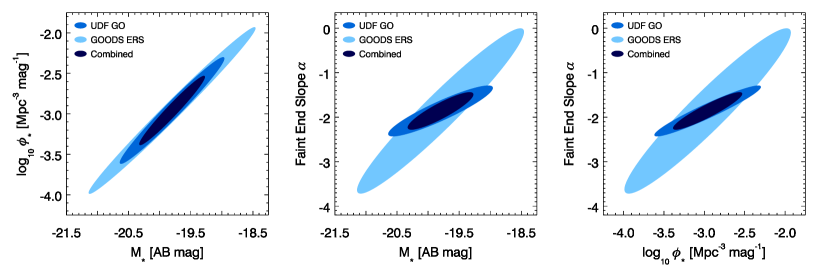
Figure 2.— Forecasted constraints on $z\sim 7$ luminosity function parameters expected from the forthcoming UDF GO and GOODS ERS WFC3 data. The constraints are calculated for a Schechter (1976) luminosity function with a characteristic luminosity $M_{\star}$, normalization $\phi_{\star}$, and faint-end slope $\alpha$. Shown are the $1-\sigma$ constraints in the $M_{\star}-\log_{10}\phi_{\star}$ (left panel), $M_{\star}-\alpha$ (middle panel), and $\log_{10}\phi_{\star}-\alpha$ (right panel) space projections for the UDF GO (blue region) and GOODS ERS (light blue region) surveys. Also shown are the constraints expected by combining both surveys (dark blue region). The depth of the UDF GO survey will provide a better constraint on the faint-end slope than GOODS ERS, but the differences between their parameter covariances make them complementary.

5.1. Forecasted Constraints for Existing Surveys

The forecasted constraints achieved by the UDF GO and GOODS ERS surveys are plotted in Figure 2. Each panel shows the constraints for the UDF GO (blue region) and GOODS ERS (light blue region) surveys separately, and in combination (dark blue region). The constraints are plotted for the $M_{\star}$-$\phi_{\star}$ (left panel), $M_{\star}$-$\alpha$ (middle panel), and $\phi_{\star}$-$\alpha$ (right panel) projections. In Figure 2 (and in similar figures throughout the paper), the shaded regions correspond to standard Gaussian contours.

Figure 2 highlights some general properties of the performance of different kinds of surveys for providing luminosity function parameter constraints, as well as specific features of the UDF GO and GOODS ERS surveys:

• The covariances between luminosity function parameters are significant and positive. In terms of the Pearson’s correlation coefficient $\rho$ for parameters $x$ and $y$, defined as

  $$\rho=\frac{C_{xy}}{\sigma_{x}\sigma_{y}},$$ (24)

  the forecasts calculate typical correlation coefficients of $\rho\gtrsim 0.9$. For a given $M_{\star}$ a narrow range of $\log_{10}\phi_{\star}$ or $\alpha$ are permitted by the data, even as the marginalized uncertainties can be as large as $\sim 30-40\%$ fractionally for $\log_{10}\phi_{\star}$ and $\alpha$.

• The orientation of the constraint ellipse forecasted for each survey can differ significantly depending on the parameter uncertainties, even if the parameter correlation coefficients for the separate surveys are similar. The orientation of the constraint ellipse major axis with respect to the $x$-axis in the $x$-$y$ parameter plane can be characterized by the angle

  $$\Theta\equiv\frac{1}{2}\arctan\left[\frac{2\rho\sigma_{x}\sigma_{y}}{\sigma_{x}^{2}-\sigma_{y}^{2}}\right]=\frac{1}{2}\arctan\left[\frac{2C_{xy}}{C_{xx}-C_{yy}}\right],$$ (25)

  which depends on the correlation $\rho$ and the parameter uncertainties. If the angle $\Theta$ differs between separate surveys, then the constraints achieved by combining the surveys can improve dramatically.

For reference, the calculated marginalized and unmarginalized errors for $\mathbf{p}$ as well as the Pearson’s correlation coefficient $\rho$ and the angle $\Theta$ for each pair of parameters are listed for the existing surveys in Table LABEL:table:existing_survey_constraints.

As Figure 2 and Table LABEL:table:existing_survey_constraints show, the UDF GO and GOODS ERS surveys will already provide interesting constraints on the abundance of $z\sim 7$ galaxies. When combined, the unmarginalized uncertainties on the LF parameters will be $\Delta M_{\star}\sim 0.1$ mag, $\Delta\log_{10}\phi_{\star}\lesssim 0.1$, and $\Delta\alpha\sim 0.15$. For the full UDF GO survey, we find that the ummarginalized uncertainty for the faint-end slope is $\Delta\alpha\sim 0.16$. Using a single UDF GO field and a limiting depth of $F160W\sim 29$ AB for a single pointing, Oesch et al. (2010b) report a faint-end slope uncertainty of $\Delta\alpha\sim 0.33$ when $\phi_{\star}$ and $M_{\star}$ are fixed (i.e., the unmarginalized uncertainty on $\alpha$). If we use the same single pointing area and depth, and the same cosmology, our estimate of the unmarginalized uncertainty would increase to $\Delta\alpha\sim 0.26$. The GOODS ERS and UDF GO surveys are complementary in that the depth of the UDF GO survey provides a beneficial constraint on the faint-end slope $\alpha$. This UDF GO constraint on $\alpha$ rotates the UDF GO error ellipse relative to the GOODS ERS constraint in the $M_{\star}-\alpha$ and $\phi_{\star}-\alpha$ projections, thereby reducing the corresponding parameter uncertainties. Individually, the GOODS ERS uncertainties will be considerably larger than those obtained by the UDF GO survey, since the GOODS ERS survey lacks sufficient depth to tightly constrain the LF faint-end slope and is not wide enough to tightly constrain $M_{\star}$ or $\phi_{\star}$.

While the UDF GO and GOODS ERS surveys achieve appreciable unmarginalized constraints, the covariances between the LF parameters are large. The marginalized uncertainties calculated for the LF parameters are $\Delta M_{\star}\sim 0.5$ mag, $\Delta\phi_{\star}\sim 0.4$, and $\Delta\alpha\sim 0.4$. Accounting for covariances these marginalized parameter uncertainties correspond to a fractional uncertainty in the total number of galaxies with $M_{\mathrm{UV}}<-18$ of $\approx 25\%$, increasing to a factor of $\approx 2$ uncertainty in the total number of galaxies with $M_{\mathrm{UV}}<M_{\star}$. To improve the constraints on the number of galaxies with $M_{\mathrm{UV}}<-18$ ($M_{\mathrm{UV}}<M_{\star})$ to $\approx 5\%$ ($\approx 50\%$) would require marginalized parameter uncertainties of approximately $\Delta M_{\star}\sim 0.2$ mag, $\Delta\phi_{\star}\sim 0.2$, and $\Delta\alpha\sim 0.2$ depending on their covariances. To reach such constraints, these UDF GO and GOODS ERS surveys would need to be complemented by either wider area or deeper surveys. We now consider some fiducial model surveys that could achieve these constraints in combination with the UDF GO and GOODS ERS data.

6. Model Surveys

The complete UDF GO and GOODS ERS surveys will provide extremely interesting initial data on the abundance of $z\sim 7$ galaxies, but the marginalized uncertainties on the LF parameters achieved by those surveys will still permit uncertainties of $\sim 25\%$ in the total number of galaxies at $M_{\mathrm{UV}}\lesssim-18$. We can repeat the calculations from §5 for fiducial model surveys to illustrate what constraints wider or deeper surveys can achieve when combined with the UDF GO and GOODS ERS data.

The model surveys are designed to be appropriate for a HST Multi-Cycle Treasury Program, which can receive up to 750 orbits per HST cycle. We consider six possible model surveys that we estimate would require $450-900$ total orbits to acquire filter coverage with the WFC IR channel.

As discussed in §4, we will assume the model surveys will use the $F140W$ filter owing to its increased throughput relative to $F160W$. The sensitivity of each survey is determined by selecting a number $N_{\mathrm{orbits}}$ of orbits per pointing, assuming 46 minutes/orbit exposure time, and using the WFC3 IR channel ETC. The total number of orbits for each survey were then determined by selecting the number of fields $N_{\mathrm{fields}}$, a mosaic geometry per field, and multiplying the number of pointings in each mosaic by $N_{\mathrm{orbits}}$ (and then doubling to account for comparable coverage in a bluer WFC3 filter).

The survey models are designed to cover a large range in total area ($A_{\mathrm{tot}}\approx 14-3600$ square arcmin), field numbers ($N_{\mathrm{fields}}=1-4$), orbits per pointing ($N_{\mathrm{orbits}}=0.5-125$), limiting depth ($H_{\mathrm{AB}}\approx 27-30$), and total number of orbits ($450-900$). We design each survey to approximate possible HST WFC3 tilings of existing surveys; as such, these model surveys represent realistic extensions of existing HST and Spitzer surveys to hundreds of orbits of WFC3 coverage. Summaries of the model surveys can be found in Table 3, and are ordered by decreasing limiting depth and increasing total area. Brief descriptions of the models follow:

Table 3Model Surveys

Model	Field Mosaic	Field Geometry	$N_{\mathrm{fields}}$	Total Area	$N_{\mathrm{orbits}}$	$H$-band Depth	Total Orbits
Name	[# Point. $\times$ # Point.]	[Arcmin. $\times$ Arcmin.]	[#]	[Sq. Arcmin.]	[#]	[AB Mag.]	[#]
Survey A	$1\times 1$	2.05′$\times$ 2.27′	3	13.96	125	30.12	750
Survey B1	$5\times 7$	10.3′$\times$ 15.9′	2	325.7	8	28.62	896
Survey B2	$5\times 7$	10.3′$\times$ 15.9′	2	325.7	6	28.46	672
Survey B3	$5\times 7$	10.3′$\times$ 15.9′	2	325.7	4	28.23	448
Survey C	$4\times 13$	8.2′$\times$ 29.5′	4	967.6	2	27.84	832
Survey D	$26\times 30$	59.0′$\times$ 61.5′	1	3628.5	0.5	27.00	780

6.1. Survey A

The performance of the UDF GO survey suggests that an interesting possible survey design would be a set of narrow pencil beam surveys with sufficient depth to reach a few nJy sensitivity. Extending each of the three single WFC3 pointing UDF GO fields to $\sim 125$ orbits in F140W would achieve $H_{\mathrm{AB}}\approx 30.1$. For surveys of $\sim 10$ square arcmin total area, using $N_{\mathrm{fields}}>1$ results in a substantial reduction of sample variance (see Figure 1). The model Survey A will therefore use $N_{\mathrm{fields}}=3$, $N_{\mathrm{orbits}}=125$, and $A_{\mathrm{tot}}=13.96$ square arcmin (three WFC3 pointings), and $750$ total orbits including coverage in a bluer WFC3 filter. For calculating constraints from a combination of Survey A with existing data, we assume the Survey A fields will be able to leverage the GOODS ERS data but will duplicate the UDF GO data.

6.2. Survey B1

Another template for a model survey is deep WFC3 coverage of the GOODS survey fields. A $5\times 7$ WFC3 mosaic could cover a field of size $10.3\arcmin\times 15.9\arcmin$, similar to the GOODS fields (Giavalisco et al., 2004). Covering $N_{\mathrm{fields}}=2$ fields the size of the GOODS fields would require 70 pointings, and would cover a total area of $A_{\mathrm{tot}}=326$ square arcmin. Using $N_{\mathrm{orbits}}=8$ orbits per pointing would reach $H_{\mathrm{AB}}=28.6$ in F140W, and would require a total of 896 orbits (including coverage in a bluer WFC3 filter). Survey B1 is the most expensive survey we consider. For calculating combined constraints utilizing existing, we will combine Survey B1 with the UDF GO data but ignore the duplicated GOODS ERS F160Wdata.

6.3. Survey B2

To gain intuition about the relative value of depth and area for constraining high-redshift galaxy populations, we will consider variations of the GOODS-like survey. Survey B2 is identical to Survey B1 in number of fields and pointings, but would achieve a reduced depth of $N_{\mathrm{orbits}}=6$ orbits per pointing ($H_{\mathrm{AB}}=28.46$). The total number of orbits required for Survey B2 is 672 (including equal coverage in a bluer WFC3 filter). When determining combined constraints with existing data, we will combine Survey B2 with the UDF GO survey.

6.4. Survey B3

Same as Survey B1 and Survey B2, but to $N_{\mathrm{orbits}}=4$ orbits per pointing ($H_{\mathrm{AB}}=28.2$) depth. Survey B3 would require 448 total orbits. For combined constraints with existing data, we will combine Survey B3 with UDF GO.

6.5. Survey C

An existing survey with a combination of large area and infrared depth is the Spitzer Extended Deep Survey (SEDS; Fazio et al., 2008), which was designed to cover $0.9{~{}\mathrm{deg}}^{2}$ over five fields to 12 hour/pointing depth with the warm Spitzer Infrared Array Camera $3.6\micron$ and $4.5\micron$ channels. Exactly reproducing the SEDS survey with WFC3 would likely be prohibitively expensive, so we will instead consider a feasible WFC3 survey with a design similar in spirit to SEDS. Our SEDS-like Survey C will consist of $N_{\mathrm{fields}}=4$ fields of $4\times 13$ pointing mosaics (each of size $8.2\arcmin\times 29.5\arcmin$), for a total area $A_{\mathrm{tot}}=967.6$ square arcmin. A depth of $N_{\mathrm{orbits}}=2$ orbits per pointing ($H_{\mathrm{AB}}=27.8$) would then require 832 orbits (including equal coverage in a bluer WFC3 filter). For calculating combined constraints with existing data, we will combine Survey C with both the UDF GO and GOODS ERS fields.

6.6. Survey D

The largest HST survey to date is the equatorial Cosmic Origins Survey (COSMOS Scoville et al., 2007b), which covers $2{~{}\mathrm{deg}}^{2}$ with the ACS $I$-band. As with the SEDS-like Survey C, exactly reproducing the COSMOS survey with WFC3 would likely be prohibitively expensive. Instead, we consider a $1{~{}\mathrm{deg}}^{2}$ ($A_{\mathrm{tot}}=3629$ square arcmin) survey with a single $26\times 30$ mosaic ($59.0\arcmin\times 61.5\arcmin$) to $N_{\mathrm{orbits}}=0.5$ orbits per pointing ($H_{\mathrm{AB}}=27$) depth. Survey D is the widest and shallowest design we consider, and would require 780 orbits to complete (including equal coverage in a bluer WFC3 filter). We will combine Survey D with both the UDF GO and GOODS ERS surveys for purposes of calculating combined constraints incorporating existing data.

6.7. Field Size Comparison

We show an illustrative comparison of the existing and model survey areas in Figure 3. The UDF GO, GOODS ERS, and Surveys A, B1, B2, B3, C, and D areas are shown as white boxes overlaid on a thin $10h^{-1}\mathrm{Mpc}$ slice through a $\Lambda\mathrm{CDM}$ cosmological simulation of comoving size $L=250h^{-1}\mathrm{Mpc}$ at $z\sim 7$ (Tinker et al., 2008). The blue scale image shows the projected dark matter surface density calculated from the dark matter particle distribution of the simulation. The comoving length scale corresponding to an angle of $\theta=1{~{}\mathrm{deg}}$ at $z=7$ is $108.7h^{-1}\mathrm{Mpc}$ for the adopted WMAP5 cosmology. This comparison illustrates the characteristic angular size of large scale structures at $z\sim 7$, as well as the survey areas required to probe representative samples of the high-redshift dark matter density distribution. The separation between fields is not to scale, and model surveys incorporating different fields would likely be more widely spaced to probe statistically independent regions on the sky.

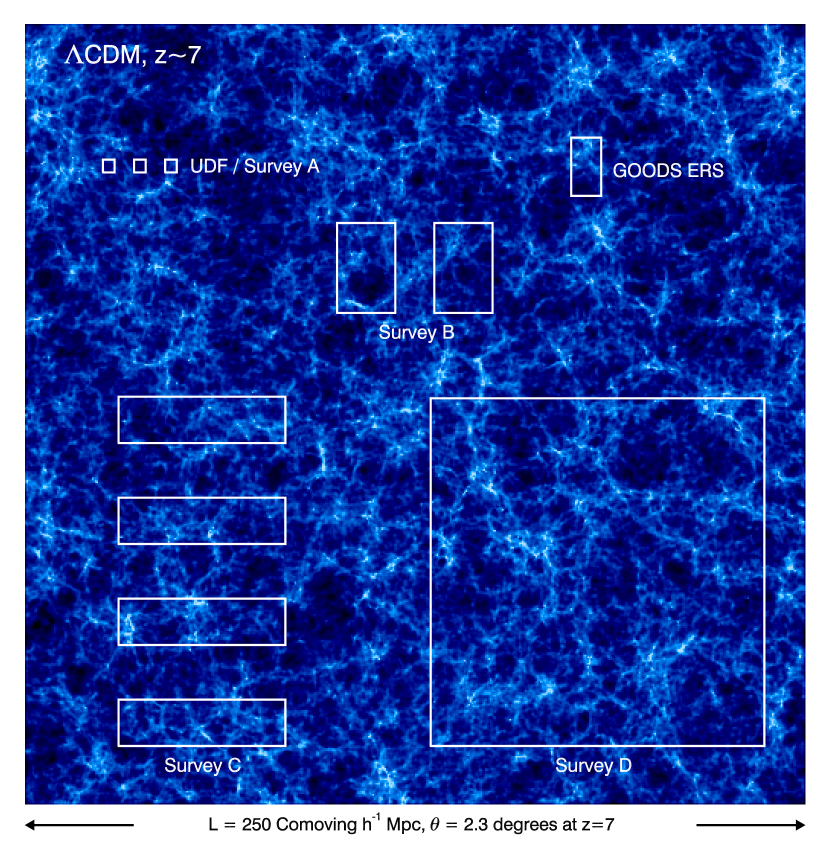
Figure 3.— Existing and model survey areas compared with the large scale dark matter structure at $z\sim 7$. Shown are the UDF GO, GOODS ERS, Surveys A, B1, B2, B3, C, and D areas (white boxes), projected onto a surface density map of a thin $10h^{-1}\mathrm{Mpc}$ slice through a $\Lambda\mathrm{CDM}$ cosmological simulation of size $L=250h^{-1}\mathrm{Mpc}$ (Tinker et al., 2008). The number of fields and survey areas of UDF GO and Survey A  are identical. This comparison illustrates the characteristic angular size of large scale structures at $z\sim 7$, as well as the survey areas required to probe representative samples of the high-redshift dark matter density distribution. The separation between fields is not to scale, and model surveys incorporating different fields would likely be more widely spaced to probe statistically independent regions on the sky.

7. Forecasted Constraints for Model Surveys

The forecasted constraints calculated for the model Surveys A, B1, B2, B3, C, and D are summarized in Table 5 and presented in Figures 4-9. In each figure, the shaded areas show the projected constraints for each model survey in the $M_{\star}-\phi_{\star}$ (left panel), $M_{\star}-\alpha$ (middle panel), and $\phi_{\star}-\alpha$ (right panel) LF parameter planes. The axes ranges in Figures 4-9 are identical (and much smaller than in Figure 2), and the plotted constraints are directly comparable. A description of the forecasted constraints for each model survey follows:

7.1. Survey A

Figure 4 shows the forecasted constraints for Survey A ($A_{\mathrm{tot}}=14$ square arcmin, $N_{\mathrm{fields}}=3$, $H_{\mathrm{AB}}=30.1$, blue region), GOODS ERS (light blue region), and GOODS ERS and Survey A combined (dark blue region). Survey A could find $>250$ $z\sim 7$ galaxies to $H_{\mathrm{AB}}\sim 30.1$, with a Poisson variance in the galaxy count of $\approx 6\%$.. The average galaxy bias for this depth and area is $\langle b\rangle\approx 5.3$, which results in a sample cosmic variance of $\sigma_{\mathrm{CV}}\approx 0.16$ fractionally. The constraints achieved by Survey A are therefore cosmic variance limited. Survey A is the deepest model survey we consider, and results in the tightest forecasted constraints on the LF faint-end slope ($\Delta\alpha\approx 0.1$, marginalized). GOODS ERS complements Survey A by providing an improved combined constraint on the LF normalization ($\Delta\phi_{\star}\approx 0.15$) and characteristic magnitude ($\Delta M_{\star}\approx 0.22$). The combined Survey A and the GOODS ERS survey also produce relatively low correlation coefficients ($\rho\approx 0.6-0.85$) compared with other surveys combinations; the orientation of the $M_{\star}-\alpha$ joint constraint from Survey A is only slightly inclined ($\Theta=12{~{}\mathrm{deg}}$), and allows the GOODS ERS survey ($\Theta=55{~{}\mathrm{deg}}$) to improve the combined constraints on $M_{\star}$.

7.2. Surveys B1, B2, and B3

These model surveys illustrate how increasing the survey limiting depth over a moderate area alter the forecasted LF parameter constraints. These surveys share a common total area ($A_{\mathrm{tot}}=326$ square arcmin) and number of fields ($N_{\mathrm{fields}}=2$), but span a factor of two in integration time ($\approx\sqrt{2}$ in sensitivity, $H_{\mathrm{AB}}=28.2-28.6$, see Table 3). Because the extra depth probes more abundant, lower-luminosity galaxies, the typical galaxy bias ($\langle b\rangle\approx 6.5$) and cosmic variance uncertainty ($\sigma_{\mathrm{CV}}\approx 0.142$) in Survey B1 would be smaller than for either Survey B2 ($\langle b\rangle\approx 6.7$, $\sigma_{\mathrm{CV}}\approx 0.146$) or Survey B3 ($\langle b\rangle\approx 7.0$, $\sigma_{\mathrm{CV}}\approx 0.152$). Similarly, the extra depth affords more observed galaxies ($N\approx 1100$) and less Poisson uncertainty ($3\%$ fractionally) for Survey B1 than for Survey B2 ($N\approx 850$, $3.4\%$) or Survey B3 ($N\approx 610$, $4.1\%$).

The Fisher matrix calculations translate the Poisson and cosmic variance uncertainties into constraints on the LF parameters, and Figures 5-7 show how the parameter constraints scale with limiting magnitude for Surveys B1, B2, and B3. In each figure, the shaded areas show the constraints achieved by UDF GO (light blue), the model surveys (blue), and the combination of UDF GO and each model survey (dark blue). The LF parameter constraints are also listed in Table 5.

Of these three surveys, Survey B1 achieves the best combined parameters constraints ($\Delta M_{\star}=0.21$, $\Delta\log_{10}\phi_{\star}=0.176$, $\Delta\alpha=0.172$). However, the relative gain over Survey B2 ($\Delta M_{\star}=0.24$, $\Delta\log_{10}\phi_{\star}=0.19$, $\Delta\alpha=0.21$) and Survey B3 ($\Delta M_{\star}=0.25$, $\Delta\log_{10}\phi_{\star}=0.21$, $\Delta\alpha=0.25$) are relatively modest ($20\%$ improvement in $\Delta M_{\star}$ and $\Delta\log_{10}\phi_{\star}$, and $40\%$ in $\Delta\alpha$). Most of the relative improvement owes to the increased constraint on the LF faint-end slope for Survey B1, since the three surveys are essentially identical for galaxies with $H_{\mathrm{AB}}<28.2$, have a similar orientation of their error ellipse in the $M_{\star}$-$\phi_{\star}$ projections ($\Theta\approx 39{~{}\mathrm{deg}}$), and have similar correlations between LF parameters. Combining with UDF GO results in a larger relative improvement in the LF parameter constraints for Survey B2 (10%) and Survey B3 (20-25%) than for Survey B1 (5%).

7.3. Survey C

The next widest model survey design is Survey C, with a total area of $A_{\mathrm{tot}}=967.6$ square arcmin to $H_{\mathrm{AB}}=27.8$ depth over $N_{\mathrm{fields}}=4$ fields. Such a survey would find $N\approx 940$ galaxies at $z\sim 7$, with an average bias of $\langle b\rangle=7.5$, cosmic variance uncertainty of $\sigma_{\mathrm{CV}}\approx 0.1$, and Poisson uncertainty of 3%.

Figure 8 shows the constraints for Survey C (blue region), the combination of UDF GO and GOODS ERS (light blue region), and the combination of all three surveys (dark blue region). The larger area of Survey C allows for better or comparable combined constraints on the LF characteristic magnitude ($\Delta M_{\star}\approx 0.19$) and normalization ($\Delta\log_{10}\phi_{\star}\approx 0.15$) than deeper surveys over smaller areas. Owing to its weaker constraint on the faint-end slope, the error ellipses provided by Survey C are more highly inclined in the $M_{\star}$-$\alpha$ ($\Theta\approx 50{~{}\mathrm{deg}}$) and $\phi_{\star}$-$\alpha$ ($\Theta\approx 59{~{}\mathrm{deg}}$) projections than the UDF GO-GOODS ERS combined constraints ($38$ and $44{~{}\mathrm{deg}}$). When combined with UDF GO and GOODS ERS surveys, Survey C would provide among the tightest constraints of the surveys we consider (with Survey A providing better combined constraints on $\alpha$ and Survey D providing better constraints on $M_{\star}$, $\phi_{\star}$, and $\alpha$).

Of additional interest for a design like Survey C is some measure of the benefit of having $N_{\mathrm{fields}}=4$ for constraining the $z\sim 7$ LF compared to a single contiguous field. We note that changing Survey C to a single field of the same total area and aspect ratio results in essentially no change to the constraints on the LF parameters (a fractional change of less than 1%). The cosmic variance uncertainty does improve by $\sim 25\%$ (see Figure 1) from $\sigma_{\mathrm{CV}}\approx 0.13$ when increasing the number of fields from $N_{\mathrm{fields}}=1$ to $N_{\mathrm{fields}}=4$, but this improvement has little net effect on the LF parameter constraints. The marginalized constraints on the LF parameters are sensitive to the Poisson errors of individual magnitude bins on the bright end of the LF, and the Poisson error is independent of $N_{\mathrm{fields}}$ for surveys of fixed total area. For magnitude bins that are Poisson-uncertainty dominated, the improvement in the cosmic sample variance gained by increasing $N_{\mathrm{fields}}$ therefore may not strongly influence end constraints on the LF parameters.

7.4. Survey D

The widest and shallowest model survey design considered is the single-field Survey D ($A_{\mathrm{tot}}\approx 1{~{}\mathrm{deg}}^{2}$, $H_{\mathrm{AB}}=27$, $N_{\mathrm{fields}}=1$). This model survey would find $N\approx 570$ galaxies at $z\sim 7$, probing only galaxies brighter than $M_{\star}$ with an average bias of $\langle b\rangle\approx 9$ with a cosmic variance uncertainty of $\sigma_{\mathrm{CV}}\approx 0.11$ (dominating over the Poisson uncertainty of $4.2\%$). Figure 9 shows the constraints that would be achieved by the combination of UDF GO and GOODS ERS  (light blue region), Survey D individually (blue region), and the combination of all three surveys (dark blue region).

The constraints achievable by Survey D individually are comparable to the constraints provided by combining UDF GO and GOODS ERS, but would require roughly three times as much additional telescope time to complete. However, the combination of Survey D with both UDF GO and GOODS ERS produces the strongest joint constraint of any survey design we considered ($\Delta M_{\star}\approx 0.136$, $\Delta\log_{10}\phi_{\star}\approx 0.11$, $\Delta\alpha\approx 0.20$). The orientation of constraint provided by Survey D individually is inclined ($\mathbf{\Theta}=[29.5,65.4,76.2]$) relative to the UDF GO-GOODS ERS combination ($\mathbf{\Theta}=[38.9,37.6,44.3]$), and results in a relatively low correlation between the LF normalization and faint-end slope ($\rho\approx 0.77$). While other survey designs produce better constraints on the faint-end slope, the joint constraint region shown in Figure 9 produces an uncertainty in the LF that is better than $\approx 6\%$ at all relatively bright ($H_{\mathrm{AB}}\lesssim 28$) magnitudes.

8. Discussion

We have considered the problem of forecasting constraints on parameters of the $z\sim 7$ LF given the characteristics of on-going surveys and models for potential future survey designs. The purview of our calculation was purposefully narrow since a more comprehensive evaluation of galaxy surveys could involve many additional questions we have not addressed. We now turn to a variety of possible caveats that stem from considering photometric galaxy survey designs more generally.

We have focused on forecasting constraints for the luminosity function. Our approach was modeled after Fisher matrix calculations that used the abundance of galaxy clusters to forecast cosmological parameters constraints (Hu & Kravtsov, 2003; Lima & Hu, 2004, 2005; Cunha & Evrard, 2009; Wu et al., 2009), but other previous calculations have forecasted cosmological parameter constraints from galaxy clustering (e.g., Vogeley & Szalay, 1996; Matsubara & Szalay, 2001, 2003; Linder, 2003; Albrecht et al., 2009). The incorporation of galaxy clustering data can circumvent some assumptions made in §2 when using simple abundance matching to assign galaxy bias by replacing the sample variance estimates in Equations 15 and 17 by an integral over the galaxy correlation function. Other estimates of how cosmic variance uncertainty is influenced by galaxy bias have taken a similar approach (e.g., Newman & Davis, 2002; Somerville et al., 2004; Stark et al., 2007b; Trenti & Stiavelli, 2008).

Our calculations have regarded a limited but interesting redshift regime near $z\sim 7$. While we have found that the combination of existing deep/narrow surveys with a future wide/shallow survey or a future ultradeep/narrow survey would provide tight constraints on the $z\sim 7$ luminosity function, studies of the galaxy population at higher and lower redshifts could require substantially different surveys. For instance, the $z\gtrsim 8$ dropout candidates identified in the UDF GO data are all fainter than $H_{\mathrm{AB}}=27.7$ (Bouwens et al., 2009; Bunker et al., 2009; McLure et al., 2010; Yan et al., 2009). The decreasing abundance of relatively bright galaxies with increasing redshift will tend to favor deeper and narrow surveys. Our calculations can easily be extended to estimate the constraining power of various surveys designs for higher-redshift galaxy populations, but we will save such estimates for future work when better fiducial estimates of the $z\gtrsim 8$ luminosity function are available.

Our Fisher matrix approach requires the use of a fiducial model for the abundance of $z\sim 7$. We adopt the Oesch et al. (2010b) estimate of the galaxy luminosity function, which was determined by scaling the characteristic magnitude $M_{\star}$ and normalization $\phi_{\star}$ from lower redshift data and then fitting for the faint-end slope $\alpha$. If the $z\sim 7$ galaxy luminosity function differs substantially from the Oesch et al. (2010b) estimate, then our forecasted constraints could be similarly inaccurate. For instance, if the normalization $\phi_{\star}$ was considerably lower or the characteristic magnitude $M_{\star}$ much fainter than that estimate by Oesch et al. (2010b), then the relative benefit of combining the UDF GO and GOODS ERS data with a wide/shallow survey over a narrow/ultradeep design could be reduced.

The calculations in §2.4.1 and §7 suggest that splitting wide surveys into multiple fields to probe statistically-independent regions of the universe may not dramatically improve constraints on the galaxy luminosity function. While this conclusion depends strongly on the total volume of the survey, other considerations such as scheduling, field observability, or sky backgrounds could make multiple fields advantageous compared with a single contiguous field of the same total area.

The abundance matching calculation also requires either knowledge or assumption about the completeness of the survey and the fraction of dark matter halos occupied by galaxies. We have assumed that the surveys are essentially volume-limited and that there is a one-to-one correspondence between galaxies and dark matter halos. Both of these assumptions are likely imperfect, and some estimates of the high-redshift occupation fraction are as low as $20\%$ (Stark et al., 2007b). The influence of these assumptions over the forecasted parameter constraints depends on the character of the survey. For a given observed luminosity function, reducing the halo occupation fraction or the survey completeness acts to reduce the effective galaxy bias in the survey by either increasing the number of halos per galaxy in the survey or increasing the number of undetected galaxies. In either case, the Poisson uncertainty is based on the observed number of galaxies and is unaffected. For purposes of constraining the observed luminosity function, wide surveys are fairly insensitive to either assumption, since Poisson uncertainty in the abundance of bright galaxies plays a large role in their error budget. The change in sample variance for narrow surveys can lead to a degradation of the marginalized parameter constraints (while the unmarginalized constraints can improve) by increasing the parameter correlations. However, the relative effect is small and the degradation is only $2\times$ for simultaneously low incompleteness ($f_{\mathrm{comp}}=0.1$) and small occupation fraction ($f_{\mathrm{occ}}=0.1$).

9. Summary

Motivated by the exciting initial galaxy survey data obtained by newly-installed Wide Field Camera 3 (WFC3) on the Hubble Space Telescope (HST), we have attempted to quantify how well on-going and possible future infrared surveys with WFC3 will constrain the abundance of galaxies at $z\sim 7$. Our primary methods and results include:

• We perform a Fisher matrix calculation to forecast constraints on the galaxy luminosity function (LF) achievable by a survey with a given depth, area, and number of fields. In our approach, the constraints on the LF normalization $\phi_{\star}$, characteristic magnitude $M_{\star}$, and faint-end slope $\alpha$ that a survey can achieve directly relate to the sample cosmic variance and Poisson uncertainty on the observed galaxy abundance through the Fisher matrix. For a fiducial LF model, the abundance of observed galaxies and dark matter halos are matched (e.g., Conroy et al., 2006; Conroy & Wechsler, 2009) to estimate the bias of galaxies of a given luminosity. The galaxy bias is combined with the RMS density fluctuations within the survey volume to calculate the sample cosmic variance (e.g., Newman & Davis, 2002; Somerville et al., 2004; Stark et al., 2007b; Trenti & Stiavelli, 2008), while the Poisson variance simply scales with the square root of the number of of observed galaxies. The constraining power of each survey is then calculated from the Fisher matrix using the Schechter (1976) model of the LF, its derivatives, the sample cosmic variance and Poisson uncertainties, and any data covariance. The combined constraints from multiple surveys can be estimated easily by summing their Fisher matrices. Similar calculations should prove useful for designing future photometric surveys and estimating their constraining power for the galaxy LF.

• Using the Fisher matrix calculations, we estimate the constraints on the abundance of $z\sim 7$ galaxies that will be achieved with the entire forthcoming Ultradeep Field Guest Observation (UDF GO) and Great Observatories Origins Deep Survey Early-Release Science (GOODS ERS) HST WFC3 IR channel data. Using the $z\sim 7$ galaxy LF estimated by Oesch et al. (2010b) as a fiducial model, we calculate that the combined UDF GO and GOODS ERS data will achieve marginalized (unmarginalized) LF parameter constraints of $\Delta M_{\star}\approx 0.5$ mag (0.1 mag), $\Delta\log_{10}\phi_{\star}\approx 0.4$ (0.1), and $\Delta\alpha\approx 0.4$ (0.15) when the surveys are fully completed. These marginalized constraints correspond to uncertainties in the total number of $z\sim 7$ galaxies with magnitudes $M_{\mathrm{UV}}<-18$ ($M_{\mathrm{UV}}<M_{\star}\approx-19.8$) of 25% (200%), after accounting for covariances between the LF parameters. These surveys will provide the first detailed information on $z\sim 7$ galaxy populations, but abundance of the bright-end of the $z\sim 7$ LF will remain uncertain without further data.

• We also forecast $z\sim 7$ LF constraints provided by a variety of model WFC3 surveys that would each require $\sim 450-900$ HST orbits. The six model surveys considered cover a large range of areas ($14-3600$ square arcmin) and depths ($H_{\mathrm{AB}}=27-30$ in $F140W$) to study the relative value area and depth for constraining the abundance of $z\sim 7$ galaxies. When combined with the forthcoming UDF GO and GOODS ERS data, all the surveys considered produce interesting luminosity function constraints (see Table 5). We find that a $\sim 1{~{}\mathrm{deg}}^{2}$ survey to $H_{\mathrm{AB}}\approx 27$ in F140W provides the tightest combined marginalized constraints ($\Delta M_{\star}\approx 0.14$, $\Delta\phi_{\star}\approx 0.11$, $\Delta\alpha\approx 0.20$) on the abundance of $z\sim 7$ galaxies of all survey designs we consider, but only by a small margin. This survey would require 780 total orbits, including equal coverage in a bluer WFC3 filter to define a drop out color selection. In contrast, the abundance of faint galaxies would be best constrained by increasing depth of the HST ultradeep fields to $\sim 125$ orbits per pointing ($H_{\mathrm{AB}}\approx 30.1$ in F140W), which provides marginalized LF constraints of $\Delta M_{\star}\approx 0.22$, $\Delta\phi_{\star}\approx 0.15$, and $\Delta\alpha\approx 0.10$ for 750 total orbits (including equal coverage in a bluer WFC3 filter).

• We also consider the usefulness of splitting surveys into $N_{\mathrm{fields}}$ multiple fields to probe independent samples and reduce cosmic variance uncertainties (e.g., Newman & Davis, 2002). We show that the shape of the $\Lambda\mathrm{CDM}$ power spectrum limits the statistical gain of splitting a high-redshift survey into multiple fields to $\lesssim 10\%$ (for $N_{\mathrm{fields}}=2$) when the survey area is large ($\gtrsim 0.5{~{}\mathrm{deg}}^{2}$). We suggest that this statistical gain should be weighed against any scientific gains achieved by probing large contiguous areas.

Initial analyses of the UDF GO data have already demonstrated that the installation of WFC3 on HST will transform our knowledge of high-redshift galaxy populations at $z\sim 7$ and beyond (e.g., Bouwens et al., 2009, 2010a, 2010b; Oesch et al., 2010b, a; Bunker et al., 2009; McLure et al., 2010; Yan et al., 2009; Wilkins et al., 2010; Labbé et al., 2009, 2010; Finkelstein et al., 2009). Our work has attempted to quantify expectations for the constraining power of the UDF GO and GOODS ERS surveys, and forecast constraints achievable with more extensive future surveys using WFC3 or other instruments. These calculations illustrate how truly powerful the refurbished HST is for exploring high-redshift galaxy populations, and emphasize how exciting near-term gains in our knowledge of $z\gtrsim 7$ galaxies will be.

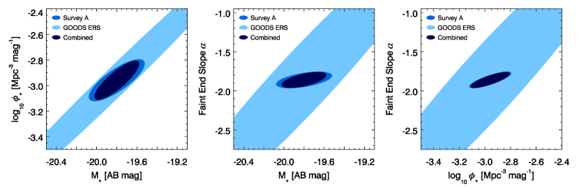
Figure 4.— Forecasted constraints on $z\sim 7$ luminosity function parameters expected from the existing GOODS ERS survey and the model Survey A. The constraints are calculated for a Schechter (1976) luminosity function with a characteristic luminosity $M_{\star}$, normalization $\phi_{\star}$, and faint-end slope $\alpha$. Shown are the $1-\sigma$ constraints in the $M_{\star}-\log_{10}\phi_{\star}$ (left panel), $M_{\star}-\alpha$ (middle panel), and $\log_{10}\phi_{\star}-\alpha$ (right panel) space projections for the GOODS ERS (light blue region) and Survey A (blue region) surveys. Also shown are the constraints expected by combining both surveys (dark blue region).

Figure 5.— Forecasted constraints on $z\sim 7$ luminosity function parameters expected from the existing UDF GO survey and the model Survey B1. The constraints are calculated for a Schechter (1976) luminosity function with a characteristic luminosity $M_{\star}$, normalization $\phi_{\star}$, and faint-end slope $\alpha$. Shown are the $1-\sigma$ constraints in the $M_{\star}-\log_{10}\phi_{\star}$ (left panel), $M_{\star}-\alpha$ (middle panel), and $\log_{10}\phi_{\star}-\alpha$ (right panel) space projections for the UDF GO (light blue region) and Survey B1 (blue region) surveys. Also shown are the constraints expected by combining both surveys (dark blue region).

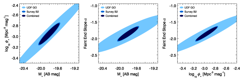
Figure 6.— Forecasted constraints on $z\sim 7$ luminosity function parameters expected from the existing UDF GO survey and the model Survey B2. The constraints are calculated for a Schechter (1976) luminosity function with a characteristic luminosity $M_{\star}$, normalization $\phi_{\star}$, and faint-end slope $\alpha$. Shown are the $1-\sigma$ constraints in the $M_{\star}-\log_{10}\phi_{\star}$ (left panel), $M_{\star}-\alpha$ (middle panel), and $\log_{10}\phi_{\star}-\alpha$ (right panel) space projections for the UDF GO (light blue region) and Survey B2 (blue region) surveys. Also shown are the constraints expected by combining both surveys (dark blue region).

Figure 7.— Forecasted constraints on $z\sim 7$ luminosity function parameters expected from the existing UDF GO survey and the model Survey B3. The constraints are calculated for a Schechter (1976) luminosity function with a characteristic luminosity $M_{\star}$, normalization $\phi_{\star}$, and faint-end slope $\alpha$. Shown are the $1-\sigma$ constraints in the $M_{\star}-\log_{10}\phi_{\star}$ (left panel), $M_{\star}-\alpha$ (middle panel), and $\log_{10}\phi_{\star}-\alpha$ (right panel) space projections for the UDF GO (light blue region) and Survey B3 (blue region) surveys. Also shown are the constraints expected by combining both surveys (dark blue region).

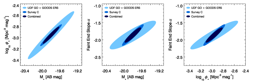
Figure 8.— Forecasted constraints on $z\sim 7$ luminosity function parameters expected from the existing UDF GO and GOODS ERS surveys and the model Survey C. The constraints are calculated for a Schechter (1976) luminosity function with a characteristic luminosity $M_{\star}$, normalization $\phi_{\star}$, and faint-end slope $\alpha$. Shown are the $1-\sigma$ constraints in the $M_{\star}-\log_{10}\phi_{\star}$ (left panel), $M_{\star}-\alpha$ (middle panel), and $\log_{10}\phi_{\star}-\alpha$ (right panel) space projections for the combined UDF GO and GOODS ERS surveys (light blue region) and the model Survey C (blue region). Also shown are the constraints expected by combining all three surveys (dark blue region).

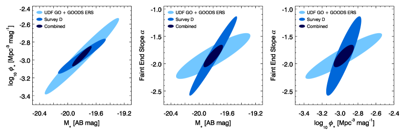
Figure 9.— Forecasted constraints on $z\sim 7$ luminosity function parameters expected from the existing UDF GO and GOODS ERS surveys and the model Survey D. The constraints are calculated for a Schechter (1976) luminosity function with a characteristic luminosity $M_{\star}$, normalization $\phi_{\star}$, and faint-end slope $\alpha$. Shown are the $1-\sigma$ constraints in the $M_{\star}-\log_{10}\phi_{\star}$ (left panel), $M_{\star}-\alpha$ (middle panel), and $\log_{10}\phi_{\star}-\alpha$ (right panel) space projections for the combined UDF GO and GOODS ERS surveys (light blue region) and the model Survey D (blue region). Also shown are the constraints expected by combining all three surveys (dark blue region).

Table 4Forecasted Constraints for Existing Surveys

Survey	Marg. Uncert.	Unmarg. Uncert.	Marg. Uncert.	Unmarg. Uncert.	Marg. Uncert.	Unmarg. Uncert.
Name	$M_{\star}$	$M_{\star}$	$\log_{10}\phi_{\star}$	$\log_{10}\phi_{\star}$	$\alpha$	$\alpha$
UDF GO	0.837	0.160	0.655	0.093	0.566	0.162
GOODS ERS	1.338	0.171	1.026	0.145	1.852	0.520
Combined	0.524	0.117	0.425	0.078	0.415	0.154
Survey	Pearson $\rho$	Pearson $\rho$	Pearson $\rho$	$\Theta(M_{\star}-\phi_{\star})$	$\Theta(M_{\star}-\alpha)$	$\Theta(\phi_{\star}-\alpha)$
Name	$M_{\star}$-$\log_{10}\phi_{\star}$	$M_{\star}$-$\alpha$	$\log_{10}\phi_{\star}$-$\alpha$	$[{~{}\mathrm{deg}}]$	$[{~{}\mathrm{deg}}]$	$[{~{}\mathrm{deg}}]$
UDF GO	0.98	0.91	0.95	38	33	41
GOODS ERS	0.99	0.96	0.95	37	55	62
Combined	0.97	0.89	0.93	39	38	44

Table 5Forecasted Constraints for Model Surveys

Survey	Marg. Uncert.	Unmarg. Uncert.	Marg. Uncert.	Unmarg. Uncert.	Marg. Uncert.	Unmarg. Uncert.
Name	$M_{\star}$	$M_{\star}$	$\log_{10}\phi_{\star}$	$\log_{10}\phi_{\star}$	$\alpha$	$\alpha$
Survey A	0.276	0.158	0.163	0.064	0.104	0.057
Survey B1	0.225	0.084	0.185	0.053	0.182	0.055
Survey B2	0.257	0.084	0.210	0.057	0.231	0.068
Survey B3	0.299	0.085	0.244	0.061	0.305	0.089
Survey C	0.244	0.052	0.193	0.041	0.311	0.088
Survey D	0.336	0.041	0.194	0.045	0.722	0.137
Ex.+Survey A	0.221	0.116	0.151	0.058	0.101	0.057
Ex.+Survey B1	0.214	0.074	0.176	0.046	0.172	0.052
Ex.+Survey B2	0.236	0.074	0.194	0.049	0.207	0.063
Ex.+Survey B3	0.253	0.075	0.210	0.051	0.245	0.078
Ex.+Survey C	0.185	0.048	0.150	0.036	0.219	0.077
Ex.+Survey D	0.136	0.039	0.111	0.039	0.201	0.103
Survey	Pearson $\rho$	Pearson $\rho$	Pearson $\rho$	$\Theta(M_{\star}-\phi_{\star})$	$\Theta(M_{\star}-\alpha)$	$\Theta(\phi_{\star}-\alpha)$
Name	$M_{\star}$-$\log_{10}\phi_{\star}$	$M_{\star}$-$\alpha$	$\log_{10}\phi_{\star}$-$\alpha$	$[{~{}\mathrm{deg}}]$	$[{~{}\mathrm{deg}}]$	$[{~{}\mathrm{deg}}]$
Survey A	0.79	0.52	0.81	28	12	30
Survey B1	0.92	0.91	0.95	39	38	45
Survey B2	0.94	0.93	0.95	39	42	48
Survey B3	0.95	0.94	0.95	39	46	52
Survey C	0.97	0.95	0.95	38	52	59
Survey D	0.96	0.97	0.90	29	65	76
Ex.+Survey A	0.84	0.62	0.82	33	18	31
Ex.+Survey B1	0.94	0.91	0.95	39	38	44
Ex.+Survey B2	0.95	0.92	0.95	39	41	47
Ex.+Survey B3	0.95	0.92	0.95	39	44	50
Ex.+Survey C	0.96	0.92	0.93	39	50	56
Ex.+Survey D	0.93	0.86	0.77	39	58	65

References

- Albrecht et al. (2009) Albrecht, A., et al. 2009, ArXiv e-prints
- Barton et al. (2004) Barton, E. J., Davé, R., Smith, J., Papovich, C., Hernquist, L., & Springel, V. 2004, ApJ, 604, L1
- Behroozi et al. (2010) Behroozi, P. S., Conroy, C., & Wechsler, R. H. 2010, ArXiv e-prints
- Bond & Myers (1996) Bond, J. R., & Myers, S. T. 1996, ApJS, 103, 1
- Bouwens et al. (2009) Bouwens, R. J., et al. 2009, ApJ, 690, 1764
- Bouwens et al. (2008) Bouwens, R. J., Illingworth, G. D., Franx, M., & Ford, H. 2008, ApJ, 686, 230
- Bouwens et al. (2010a) Bouwens, R. J., et al. 2010a, ApJ, 709, L133
- Bouwens et al. (2010b) —. 2010b, ApJ, 708, L69
- Bouwens et al. (2005) Bouwens, R. J., Illingworth, G. D., Thompson, R. I., & Franx, M. 2005, ApJ, 624, L5
- Bouwens et al. (2004) Bouwens, R. J., et al. 2004, ApJ, 616, L79
- Bradley et al. (2008) Bradley, L. D., et al. 2008, ApJ, 678, 647
- Bunker et al. (2009) Bunker, A., et al. 2009, ArXiv e-prints
- Castellano et al. (2010) Castellano, M., et al. 2010, A&A, 511, A20+
- Conroy & Wechsler (2009) Conroy, C., & Wechsler, R. H. 2009, ApJ, 696, 620
- Conroy et al. (2006) Conroy, C., Wechsler, R. H., & Kravtsov, A. V. 2006, ApJ, 647, 201
- Crocce et al. (2006) Crocce, M., Pueblas, S., & Scoccimarro, R. 2006, MNRAS, 373, 369
- Cuby et al. (2007) Cuby, J., Hibon, P., Lidman, C., Le Fèvre, O., Gilmozzi, R., Moorwood, A., & van der Werf, P. 2007, A&A, 461, 911
- Cunha & Evrard (2009) Cunha, C. E., & Evrard, A. E. 2009, ArXiv e-prints
- Davé et al. (2006) Davé, R., Finlator, K., & Oppenheimer, B. D. 2006, MNRAS, 370, 273
- Dayal et al. (2010) Dayal, P., Ferrara, A., & Saro, A. 2010, MNRAS, 402, 1449
- Dayal et al. (2009) Dayal, P., Ferrara, A., Saro, A., Salvaterra, R., Borgani, S., & Tornatore, L. 2009, MNRAS, 400, 2000
- Egami et al. (2005) Egami, E., et al. 2005, ApJ, 618, L5
- Eisenstein & Hu (1998) Eisenstein, D. J., & Hu, W. 1998, ApJ, 496, 605
- Fazio et al. (2008) Fazio, G., et al. 2008, in Spitzer Proposal ID #60022, 60022–+
- Fernandez & Komatsu (2008) Fernandez, E. R., & Komatsu, E. 2008, MNRAS, 384, 1363
- Finkelstein et al. (2009) Finkelstein, S. L., Papovich, C., Giavalisco, M., Reddy, N. A., Ferguson, H. C., Koekemoer, A. M., & Dickinson, M. 2009, ArXiv e-prints
- Fisher (1935) Fisher, R. A. 1935, Journal of the Royal Statistical Society, 98, 39
- Freedman et al. (2001) Freedman, W. L., et al. 2001, ApJ, 553, 47
- Furlanetto et al. (2006) Furlanetto, S. R., Zaldarriaga, M., & Hernquist, L. 2006, MNRAS, 365, 1012
- Giavalisco et al. (2004) Giavalisco, M., et al. 2004, ApJ, 600, L93
- Gonzalez et al. (2010) Gonzalez, V., Labbe, I., Bouwens, R. J., Illingworth, G., Franx, M., Kriek, M., & Brammer, G. B. 2010, ApJ in press
- Gottlöber & Yepes (2007) Gottlöber, S., & Yepes, G. 2007, ApJ, 664, 117
- Gunn & Gott (1972) Gunn, J. E., & Gott, J. R. I. 1972, ApJ, 176, 1
- Haiman (2002) Haiman, Z. 2002, ApJ, 576, L1
- Hansen & Oh (2006) Hansen, M., & Oh, S. P. 2006, MNRAS, 367, 979
- Henry et al. (2008) Henry, A. L., Malkan, M. A., Colbert, J. W., Siana, B., Teplitz, H. I., & McCarthy, P. 2008, ApJ, 680, L97
- Henry et al. (2007) Henry, A. L., Malkan, M. A., Colbert, J. W., Siana, B., Teplitz, H. I., McCarthy, P., & Yan, L. 2007, ApJ, 656, L1
- Henry et al. (2009) Henry, A. L., et al. 2009, ApJ, 697, 1128
- Hibon et al. (2009) Hibon, P., et al. 2009, AA in press
- Hickey et al. (2010) Hickey, S., Bunker, A., Jarvis, M. J., Chiu, K., & Bonfield, D. 2010, MNRAS in press
- Holder et al. (2001) Holder, G., Haiman, Z., & Mohr, J. J. 2001, ApJ, 560, L111
- Hu & Cohn (2006) Hu, W., & Cohn, J. D. 2006, Phys. Rev. D, 73, 067301
- Hu & Kravtsov (2003) Hu, W., & Kravtsov, A. V. 2003, ApJ, 584, 702
- Iye et al. (2006) Iye, M., et al. 2006, Nature, 443, 186
- Kaiser (1984) Kaiser, N. 1984, ApJ, 284, L9
- Kashikawa et al. (2006) Kashikawa, N., et al. 2006, ApJ, 648, 7
- Kitzbichler & White (2007) Kitzbichler, M. G., & White, S. D. M. 2007, MNRAS, 376, 2
- Kneib et al. (2004) Kneib, J., Ellis, R. S., Santos, M. R., & Richard, J. 2004, ApJ, 607, 697
- Kobayashi et al. (2007) Kobayashi, M. A. R., Totani, T., & Nagashima, M. 2007, ApJ, 670, 919
- Kobayashi et al. (2010) —. 2010, ApJ, 708, 1119
- Kodaira et al. (2003) Kodaira, K., et al. 2003, PASJ, 55, L17
- Komatsu et al. (2009) Komatsu, E., et al. 2009, ApJS, 180, 330
- Kowalski et al. (2008) Kowalski, M., et al. 2008, ApJ, 686, 749
- Kravtsov et al. (2004) Kravtsov, A. V., Berlind, A. A., Wechsler, R. H., Klypin, A. A., Gottlöber, S., Allgood, B., & Primack, J. R. 2004, ApJ, 609, 35
- Labbé et al. (2009) Labbé, I., et al. 2009, ArXiv e-prints
- Labbé et al. (2010) —. 2010, ApJ, 708, L26
- Le Delliou et al. (2006) Le Delliou, M., Lacey, C. G., Baugh, C. M., & Morris, S. L. 2006, MNRAS, 365, 712
- Lee et al. (2009) Lee, K., Giavalisco, M., Conroy, C., Wechsler, R. H., Ferguson, H. C., Somerville, R. S., Dickinson, M. E., & Urry, C. M. 2009, ApJ, 695, 368
- Lima & Hu (2004) Lima, M., & Hu, W. 2004, Phys. Rev. D, 70, 043504
- Lima & Hu (2005) —. 2005, Phys. Rev. D, 72, 043006
- Linder (2003) Linder, E. V. 2003, Phys. Rev. D, 68, 083504
- Mao et al. (2007) Mao, J., Lapi, A., Granato, G. L., de Zotti, G., & Danese, L. 2007, ApJ, 667, 655
- Matsubara & Szalay (2001) Matsubara, T., & Szalay, A. S. 2001, ApJ, 556, L67
- Matsubara & Szalay (2003) —. 2003, Physical Review Letters, 90, 021302
- McLure et al. (2010) McLure, R. J., Dunlop, J. S., Cirasuolo, M., Koekemoer, A. M., Sabbi, E., Stark, D. P., Targett, T. A., & Ellis, R. S. 2010, MNRAS, 126
- McQuinn et al. (2007) McQuinn, M., Hernquist, L., Zaldarriaga, M., & Dutta, S. 2007, MNRAS, 381, 75
- Mesinger & Furlanetto (2008) Mesinger, A., & Furlanetto, S. R. 2008, MNRAS, 386, 1990
- Mo & White (1996) Mo, H. J., & White, S. D. M. 1996, MNRAS, 282, 347
- Muñoz & Loeb (2008) Muñoz, J. A., & Loeb, A. 2008, MNRAS, 386, 2323
- Muñoz et al. (2009) Muñoz, J. A., Trac, H., & Loeb, A. 2009, ArXiv e-prints
- Newman & Davis (2002) Newman, J. A., & Davis, M. 2002, ApJ, 564, 567
- Nilsson et al. (2007) Nilsson, K. K., Orsi, A., Lacey, C. G., Baugh, C. M., & Thommes, E. 2007, A&A, 474, 385
- Oesch et al. (2010a) Oesch, P. A., et al. 2010a, ApJ, 709, L21
- Oesch et al. (2010b) —. 2010b, ApJ, 709, L16
- Oesch et al. (2009) —. 2009, ApJ, 690, 1350
- Oke & Gunn (1983) Oke, J. B., & Gunn, J. E. 1983, ApJ, 266, 713
- Ota et al. (2008) Ota, K., et al. 2008, ApJ, 677, 12
- Ouchi et al. (2009a) Ouchi, M., et al. 2009a, ApJ, 706, 1136
- Ouchi et al. (2009b) —. 2009b, ApJ, 696, 1164
- Parkes et al. (1994) Parkes, I. M., Collins, C. A., & Joseph, R. D. 1994, MNRAS, 266, 983
- Peacock & Dodds (1996) Peacock, J. A., & Dodds, S. J. 1996, MNRAS, 280, L19
- Percival et al. (2007) Percival, W. J., Cole, S., Eisenstein, D. J., Nichol, R. C., Peacock, J. A., Pope, A. C., & Szalay, A. S. 2007, MNRAS, 381, 1053
- Richard et al. (2006) Richard, J., Pelló, R., Schaerer, D., Le Borgne, J., & Kneib, J. 2006, A&A, 456, 861
- Richard et al. (2008) Richard, J., Stark, D. P., Ellis, R. S., George, M. R., Egami, E., Kneib, J., & Smith, G. P. 2008, ApJ, 685, 705
- Samui et al. (2009) Samui, S., Srianand, R., & Subramanian, K. 2009, MNRAS, 398, 2061
- Santos (2004) Santos, M. R. 2004, MNRAS, 349, 1137
- Santos et al. (2004) Santos, M. R., Ellis, R. S., Kneib, J., Richard, J., & Kuijken, K. 2004, ApJ, 606, 683
- Schechter (1976) Schechter, P. 1976, ApJ, 203, 297
- Scoville et al. (2007a) Scoville, N., et al. 2007a, ApJS, 172, 38
- Scoville et al. (2007b) —. 2007b, ApJS, 172, 1
- Sheth et al. (2001) Sheth, R. K., Mo, H. J., & Tormen, G. 2001, MNRAS, 323, 1
- Sheth & Tormen (1999) Sheth, R. K., & Tormen, G. 1999, MNRAS, 308, 119
- Smith et al. (2003) Smith, R. E., et al. 2003, MNRAS, 341, 1311
- Sobral et al. (2009) Sobral, D., et al. 2009, MNRAS, 398, L68
- Somerville et al. (2004) Somerville, R. S., Lee, K., Ferguson, H. C., Gardner, J. P., Moustakas, L. A., & Giavalisco, M. 2004, ApJ, 600, L171
- Springel et al. (2005) Springel, V., et al. 2005, Nature, 435, 629
- Stanway et al. (2008) Stanway, E. R., Bremer, M. N., Squitieri, V., Douglas, L. S., & Lehnert, M. D. 2008, MNRAS, 386, 370
- Stark & Ellis (2006) Stark, D. P., & Ellis, R. S. 2006, New Astronomy Review, 50, 46
- Stark et al. (2007a) Stark, D. P., Ellis, R. S., Richard, J., Kneib, J., Smith, G. P., & Santos, M. R. 2007a, ApJ, 663, 10
- Stark et al. (2007b) Stark, D. P., Loeb, A., & Ellis, R. S. 2007b, ApJ, 668, 627
- Taniguchi et al. (2005) Taniguchi, Y., et al. 2005, PASJ, 57, 165
- Tasitsiomi (2006) Tasitsiomi, A. 2006, ApJ, 645, 792
- Tegmark et al. (1997) Tegmark, M., Taylor, A. N., & Heavens, A. F. 1997, ApJ, 480, 22
- Tilvi et al. (2009) Tilvi, V., Malhotra, S., Rhoads, J. E., Scannapieco, E., Thacker, R. J., Iliev, I. T., & Mellema, G. 2009, ApJ, 704, 724
- Tinker et al. (2008) Tinker, J., Kravtsov, A. V., Klypin, A., Abazajian, K., Warren, M., Yepes, G., Gottlöber, S., & Holz, D. E. 2008, ApJ, 688, 709
- Tinker et al. (2010) Tinker, J. L., Robertson, B. E., Kravtsov, A. V., Klypin, A., Warren, M. S., Yepes, G., & Gottlober, S. 2010, ArXiv e-prints
- Trenti & Stiavelli (2008) Trenti, M., & Stiavelli, M. 2008, ApJ, 676, 767
- Vogeley & Szalay (1996) Vogeley, M. S., & Szalay, A. S. 1996, ApJ, 465, 34
- Warren et al. (2006) Warren, M. S., Abazajian, K., Holz, D. E., & Teodoro, L. 2006, ApJ, 646, 881
- Wilkins et al. (2010) Wilkins, S. M., Bunker, A. J., Ellis, R. S., Stark, D., Stanway, E. R., Chiu, K., Lorenzoni, S., & Jarvis, M. J. 2010, MNRAS, 176
- Willis & Courbin (2005) Willis, J. P., & Courbin, F. 2005, MNRAS, 357, 1348
- Willis et al. (2008) Willis, J. P., Courbin, F., Kneib, J., & Minniti, D. 2008, MNRAS, 384, 1039
- Wu et al. (2009) Wu, H., Zentner, A. R., & Wechsler, R. H. 2009, ArXiv e-prints
- Wyithe & Loeb (2005) Wyithe, J. S. B., & Loeb, A. 2005, ApJ, 625, 1
- Yan et al. (2009) Yan, H., Windhorst, R., Hathi, N., Cohen, S., Ryan, R., O’Connell, R., & McCarthy, P. 2009, ArXiv e-prints
- Yepes et al. (2007) Yepes, G., Sevilla, R., Gottlöber, S., & Silk, J. 2007, ApJ, 666, L61
- Zheng et al. (2009) Zheng, W., et al. 2009, ApJ, 697, 1907