The chromosphere: gateway to the corona?

Abstract

I argue that one should attempt to understand the solar chromosphere not only for its own sake, but also if one is interested in the physics of: the corona; astrophysical dynamos; space weather; partially ionized plasmas; heliospheric UV radiation; the transition region. I outline curious observations which I personally find puzzling and deserving of attention.

1 Introduction

A cursory glance at the literature reveals that chromospheres are something of an astronomical backwater. Of $10^{6}$ abstracts listed in the ADS (astrophysics section) between 2000 and July 2009, a mere $4.5\times 10^{3}$ have chromosphere in the abstract, slightly less than planetary nebulae and only twice the number of papers of something entirely invisible, dark matter. Its repugnance presumably lies in the difficult regimes of non-LTE and non-ionization equilibrium, equipartition of magnetic and dynamical energies, its awesome fine scale structure, as well as other potential horror stories involving its poorly understood connections to the photosphere and corona.

Why, then, should anyone be interested in it? Here I attempt to show why we can no longer just “brush the chromosphere under the carpet”, (magnetic or figurative) and ignore its importance either in a solar or plasma physics context. I hope to convince the reader that the chromosphere deserves to be studied by more than an interesting group of souls who have, like myself, long since lost their way, and become hopelessly entangled in one of the most awkward parts of the Sun. The paper discusses also several problems shamelessly of interest to the present author, narrated with the help of architypal “lost soul” Edgar Allen Poe, whose bicentennial birthday anniversary is 2009.

Readers looking for a respectable review from an observational perspective can look to Rutten (2006), a somewhat historical viewpoint is given by Judge (2006), and recent exciting results can be found in papers in the present volume.

2 Seven reasons why the chromosphere is important

In the late 1800s, Hale and Deslandres independently developed and applied the spectroheliograph to lines of Ca II, known from eclipses to be prominent in the solar chromosphere. Hale & Ellerman’s (1904) photographic spectroheliograms of the disk chromosphere revealed the “chromospheric network” at various wavelengths in the Ca II $H$ and $K$ lines and in H$\beta$, and showed that enhanced chromospheric emission occurs in “clouds” or “flocculi” above photospheric faculae. In the 1950s, the bright network discovered was found to be correlated with photospheric velocity and magnetic fields, associated with supergranular motions identified by (Simon & Leighton, 1963, 1964). The chromosphere is the source of variable UV irradiation. Since the visual work of Secchi in the 1870s, the chromosphere seen in light of H$\alpha$ (the rose colored line responsible for the chromosphere’s name) was known to contain remarkable and beautiful fine structure (network, fibrils, spicules). In the 1960s, slit spectra with film and electronic detectors revealed that the chromosphere is dynamic, supporting wave motions as well as spicules, dynamic fibrils, surges etc. Thus I come to the first two reasons to study the chromosphere:

1: We do not understand from first principles why the Sun is obliged to manifest these phenomena.

2: Variable UV influences the heliosphere, including the Earth’s atmosphere.

A third simple reason is

3: The Sun is not alone.

Chromospheres are present whenever a star possesses a convection zone. Beginning in the 1960s, Olin Wilson began monitoring stellar chromospheric emission in the cores of the Ca II resonance lines (Wilson, 1978). This record continues today and serves as the prime database by which stellar activity cycles, manifestations of dynamo action observed in the Sun, can be studied (Baliunas et al., 1995; Lockwood et al., 2007). This is because magnetic fields on the surfaces of convective stars lead to network and plage heating, directly reflected in chromospheric emission. More direct measurements of magnetic fields for solar-like stars are very difficult, essentially because there are no magnetic monopoles and the signals in polarized light cancel almost completely, when integrated over the stellar surface . Thus we have reason number

4: Variable chromospheric emission sheds light on dynamo properties across the HR diagram.

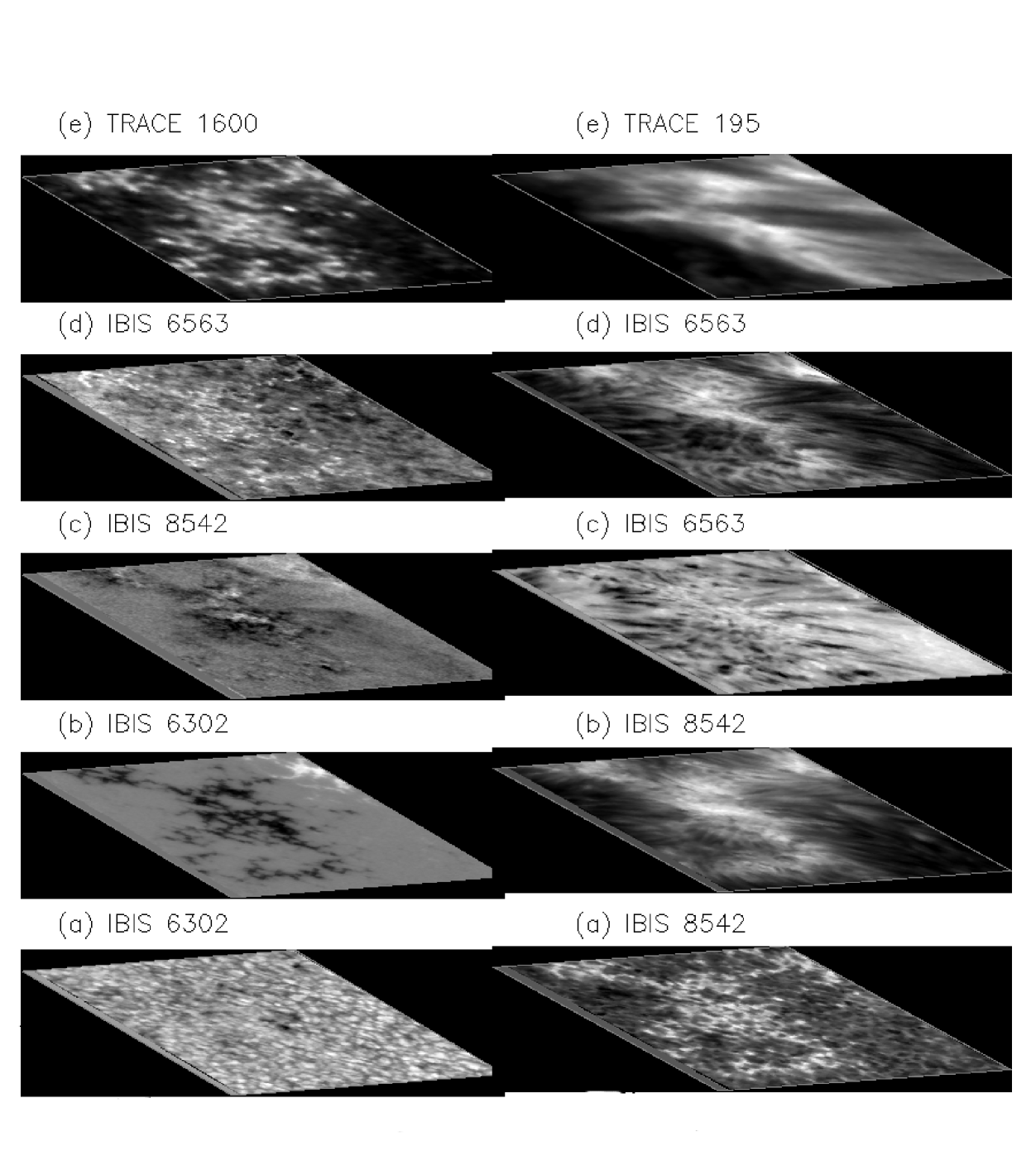
Figure 1: Joint observations of pores from IBIS and TRACE from 20 May 2008 (Judge et al., in preparation). The left hand panels show (a) the photospheric continuum near 630.2 nm, (b) and (c) “magnetograms” in the photosphere and chromosphere respectively, (d) far wing of H$\alpha$, (e) 160 nm continuum from TRACE. The right panels show (a) wing of Ca II 854.2 nm, (b) core of 854.2, (c) and (d) H$\alpha$ 0.8 and 0.1 Å blueward of line center, (e) TRACE 19.5 nm coronal loops and footpoints. The field of view is 32 Mm on a side. The fibril structure, requiring $\sim 1\arcsec$ resolution to see clearly, of both H$\alpha$ and Ca II 854.2 nm chromospheric lines, outlines the morphology of the base of the overlying corona.

The structure of the solar corona is imprinted already the chromosphere, something seen clearly when when chromospheric fibrils/spicules are resolved. This chromospheric “fine structure” (e.g. Secchi, 1877; Kiepenheuer, 1953; Athay, 1976) is now known to bear similarities in morphology and dynamics to the overlying corona. Figure 1 shows an example of one part of a small bipolar active region – the difference in physical conditions photospheric and coronal images is striking. The morphology of images obtained near the H$\alpha$ line core is most simply understood as reflecting a cool component of the low-$\beta$ hydromagnetic system, which extends into the overlying corona. Being dependent on unknown terms in the energy equation, it is not understood what leads to the mix of cool and hot material that is represented by such data. This aside, the important thing is that hydromagnetic conditions at the coronal base can in principle be diagnosed using upper chromospheric lines. The low-$\beta$ state of the upper chromosphere, inferred simply from the morphology (and dynamics) of fine structure, implies that it is in a (nearly) force-free state. Magnetic field measurements made there lead us to reasons number

5: Meaningful force-free boundary conditions can be used for extrapolations into the corona, and

6: Using the magnetic virial theorem (Chandrasekhar, 1961), the free energy can in principle be determined in the overlying coronal volume.

Chandrasekhar’s theorem applied to volume $V$ bounded by surface $S$ with normal s can be written

$$\int_{V}{\bf r\cdot[(\nabla\times B)\times B]}dV=$$

$$\int_{V}\frac{1}{2}B^{2}dV+\int_{S}[({\bf B\cdot r}){\bf B}-\frac{1}{2}B^{2}{\bf r}]\cdot d{\bf s}.$$ (1)

When ${\bf j=\nabla\times B=0}$, the LHS vanishes, and the result follows. Consider a volume of the Sun’s atmosphere, in a low-$\beta$ state, bounded by the chromosphere at the base and by force-free conditions extending into the corona itself. Measurements of the vector field in $S$ then suffice to determine the total integrated magnetic energy, from which the potential energy from the surface may be subtracted. The application of chromospheric lines in this manner has not yet been realized, but steps are being taken (e.g. Judge et al., 2010b).

Presently unknown chromospheric physics serves to modulate the flow of mass, momentum, energy into the corona (Holzer et al., 1997). Indeed, it is the mass reservoir required for “coronal loop scaling laws” (e.g. Rosner et al., 1978; Jordan, 1992). But the chromosphere also modulates the magnetic field as it emerges into the corona, in two ways. First, force balance requires that ${\bf|j\times B|\rightarrow 0}$ above the $\beta=1$ surface which, outside of umbrae and very quiet Sun, lies within the chromosphere. Second, ion-neutral collisions selectively dissipate components of ${\bf j}$, ${\bf j_{\perp}}$, perpendicular to ${\bf B}$, with significant consequences for the nature and stability of emerged magnetic flux (Leake & Arber, 2006; Arber et al., 2007, 2009). Thus we are led to reason

7: The chromosphere actively sets the boundary conditions for the corona and its evolution.

The ion-neutral collisions dissipate magnetic energy more efficiently when the magnetic fluctuations have higher frequencies, thus the chromosphere serves as a low-pass filter for certain kinds of magnetic fluctuations (e.g. de Pontieu & Haerendel, 1998), reducing any high frequency photospheric fluctuations from the spectrum of fluctuations surviving to the corona. Further discussion of these points is found in a review by Judge (2009) .

That I arrived at the number seven – the number of deadly sins – came as a surprise. The deadly sins were rendered a thing of heavenly beauty in oil on wood by Hieronymous Bosch in 1485, inscribed “Beware, Beware, God Sees”. Perhaps Helios is telling the author something. Perhaps not. In any case the chromosphere’s secrets made manifest will surely be a heavenly, not hellish, revelation for solar physics.

3 Current chromospheric challenges

The chromosphere is of course interesting in its own right, and much research is rightly focused on aspects of my “reason number 1”. Here I take the editors’ advice and author’s prerogative to again step back and look at curious aspects of the magnetized chromosphere – why the chromosphere has bright network and plage emission, why they behave as they do, and how the transition region may fit into the picture. I take it as given that the chromosphere is controlled by (sub-) photospheric dynamics, including convective and wave motions, and by the emergence and transport of magnetic fields into strong supergranular downflow lanes, thereby producing the network pattern.

3.1 “The Purloined Letter”

Poe’s (1844) iconoclastic detective story reminds me of recent observations of the solar limb from the Hinode spacecraft. How so? Well in both cases detectives searched high and low, but their search has missed something. In Poe’s story, a letter is in plain sight. In the Sun, the (non-spicule) chromosphere must be present and in fact dominant in terms of mass, but is so notably missing from the data that it is obvious by its absence. Where is the limb chromosphere?

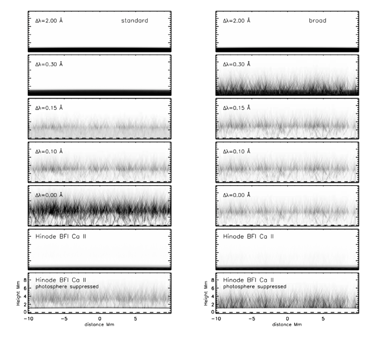
Figure 2: Intensities computed at several monochromatic wavelengths and in the Hinode BFI passband are shown as a function of position along the limb tangential direction and radial height. The color table is reversed for clarity: bright intensity=dark images. “Standard” spicule conditions were applied in which spicules have the same line profiles as the ambient inter-spicule medium (left panel), and broad spicular emission lines were computed (right panel). Observations are qualitatively similar to the “broad” calculation.

The BFI instrument on Hinode, fed by the Solar Optical Telescope (SOT Tsuneta et al., 2008), has been used to observe the H line of Ca II using a 3 Å wide spectral bandpass ($\equiv 230$ km s^-1). At and near the solar limb, such data are characterized by what appears to be a remarkably dynamic, spicule-dominated chromosphere at the limb of the Sun (e.g. de Pontieu et al., 2007). Little or no absorption of spicule light is seen along their lengths. Judge & Carlsson (2010, in preparation) present formal solutions to the transfer equation for given (ad-hoc) source functions, including an ambient stratified chromosphere from which spicules originate. Now, some absorption must be expected because there must be material with significant opacity in the Ca II lines between the photosphere and corona, that is not within the spicule population. Evidence for such material is plentiful and contained, for example, in disk observations of the internetwork chromosphere (e.g. Lites et al., 1993). Figure 2 shows two calculations from Judge & Carlsson’s formal solutions, the lowest panels showing observables computed for the BFI. On the basis of these calculations, Judge & Carlsson argue that the Hinode data require the observed spicule emission to be significantly Doppler shifted compared with the ambient atmosphere, either by turbulent or organized spicular motions. According to Judge & Carlsson, at the limb, the broad bandpass of the Hinode BFI instrument preferentially detects the bright, dynamic structures whose line widths and Doppler shifts are sufficient to avoid the absorption by the intervening material. The non-spicule chromosphere, the stratified layer between the photosphere and corona which must be present, is difficult to see in these data.

The consequences of “not seeing the Purloined Letter” are perhaps significant. Using standard estimates (Athay & Holzer, 1982; Vernazza et al., 1981, “VAL”), the total spicule type II mass is only $10^{-4}$ to $10^{-5}$ of the mass of the entire chromosphere- spicules have a far smaller filling factor and density than the chromospheric base. Within a network element, the enthalpy flux density is a factor of several lower than the radiative flux density of $\geq 2\times 10^{7}$ erg cm^-2 s^-1 of the network chromosphere (“guestimated” from VAL , using losses including Fe II lines from Anderson & Athay, 1989). I conclude that the spicules observed comprise a small mass and energy fraction of the chromosphere, the bulk of which remains unseen by filter instruments like the BFI on Hinode. They are important, however, in that they present a large areal interface to the corona which will be mentioned below (section 3.3). They appear to supply large amounts of mass to the corona (Athay & Holzer, 1982), and they reveal Alfvénic fluctuations as they propagate magnetic wave energy into the corona (de Pontieu et al., 2007).

3.2 “The Cask of Amontillado”

The network chromosphere exhibits a property which, to the present author, is a curiosity. The bright network emission remains geometrically confined to overlie the photospheric magnetic field concentrations, yet the magnetic field where the chromospheric emission is bright must expand rapidly with height. Figure 2 shows very narrow band images obtained using the Echelle spectrograph at the Vacuum Tower Telescope by Rammacher et al. (2008).

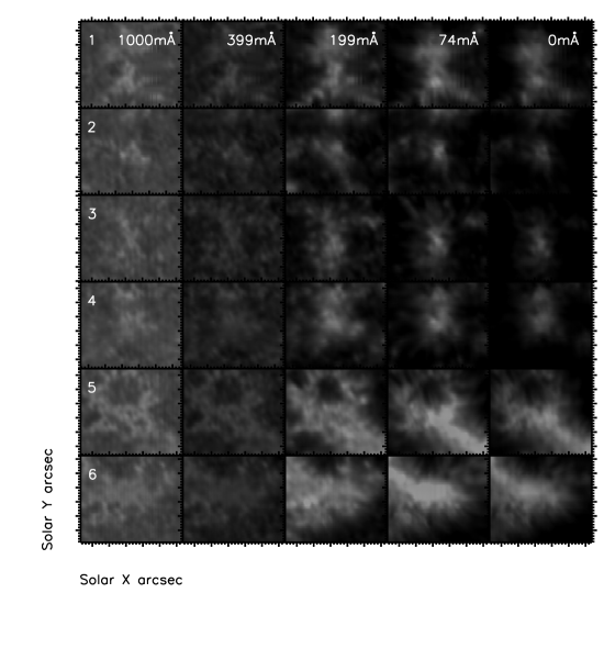
Figure 3: Images constructed from Echelle spectrograph observations from June 13 2007, binned over 22.5 mÅ, are shown for several different regions of network emission (labeled 1-6). The intensity scales are are the same scale for all images. Each region is $30\arcsec\times 30\arcsec$ in size, on the order of a typical supergranule cell size. Along each row the wavelength varies from wing to line center, thus the rightmost images are formed highest in the chromosphere.

The figure shows that the Ca II emission remains remarkably confined locally over the photospheric flux concentrations, yet the emission comes from regions spanning several pressure scale heights.

Natural explanations exist to explain why both bright photospheric and transition region plasmas are locally confined to the network boundaries. However, Judge et al. (2010a) note that there is a potential problem for force balance in the chromosphere, in essence because bright emission usually requires higher gas pressures. Empirical bright network models (VAL-like) have a higher gas pressure at each geometric height than cell interior models; the plasma pressure is expected to exceed the magnetic pressure at least somewhere in the network chromosphere, and the magnetic pressure is far higher over the network boundary. The chromosphere has time to equilibrate pressures from network boundary to cell interior (several tens of minutes) on the life time of supergranular structures (30 hours or so). So, horizontal pressure equilibrium is a reasonable approximation, yet the above data show that bright emission is steadfastly confined to regions close to the network boundary. How can this be?

A “resolution” of this apparent conundrum is to lower empirical (VAL-like) models down by the couple of scale heights needed to achieve force balance within the photosphere (Solanki et al., 1991). But the present author considers their success as a real surprise given that the VAL models (1) are identical in the underlying photosphere, and (2) were constructed to match spatially averaged intensities in the much higher chromosphere which do not completely resolve the network. There is no physical reason why this drop in height naturally should lead to force balance in the chromosphere- the height drop is determined entirely by photospheric physics, because the overlying chromospheric conditions are determined by processes occurring some 5-9 scale heights higher up. While there is of course a physical link between these layers, the author is truly amazed that the VAL stratification simply slid downwards can accommodate chromospheric force balance, something that is not guaranteed in such modeling efforts.

Poe’s (1846) short story “The Cask of Amontillado” is concerned with immurement – being imprisoned between walls. Judge et al. (2010a) ask if something is missing in our understanding of the force and energy balance of the chromosphere, or is the network chromosphere immured by some forces yet to be identified?

3.3 “The Fall of the House of Usher”

Summarizing the 1994 NSO Summer Workshop, Eugene Parker commented on the “horror of the solar transition region”, in reference to a work claiming that it consists of filamentary structure filling tiny fractions of the available volume (e.g. Dere et al., 1987; Judge & Brekke, 1994). The author has a feeling that the latter paper and perhaps other transition region (TR) literature fits one of Poe’s genres: “horror fiction”. The TR has the (un-?) fortunate property of radiating a lot of UV radiation at wavelengths where (1) the background continuum is relatively weak (wavelengths below 165 nm), and (2) normal incidence spectrographs are highly reflective (wavelengths above 115 nm). It is also “sandwiched” between the chromosphere and corona, contains very little mass, and so tends to be spectacularly responsive to perturbations both from the underlying chromosphere and the overlying corona. Being, then, a prime target for interesting observations, the literature measured by solar-stellar “transition region” articles in the ADS constitutes almost 40 % of that for the literature chromosphere which spans 9 scale heights and contains 5 orders of magnitude more mass.

The story of explaining the lower TR and its connection to the chromosphere perhaps has parallels with Poe’s “The House of Usher”, a tale with dramatic imagination but with tragically flawed characters. The house itself and its inhabitants, a brother and sister with psychological problems, are ultimately finished off by a bolt of lightning. No flash of brilliance has yet brought the transition region story to an end, but many imaginative physical pictures have been brought to bear on the problem.

In the 1970s C. Jordan pointed out that resonance lines of neutral and ionized helium, formed in the lower TR are factors of several too bright compared with other lines, without the need for models (Jordan, 1975). Judge et al. (1995) showed that a similar problem existed for Li and Na-like ions, using highly accurate irradiance data. In a step perhaps towards insanity, one wonders if the basic assumptions behind such emission measure work are valid for any TR line. Models dominated by heat conduction produce too little emission from the lower TR (below $2\times 10^{5}$ K) by orders of magnitude, unless somewhat special and questionable geometries are invoked to allow cross-field (ion-dominated) heat conduction to occur (Athay, 1990). This serious problem was evident early (Athay, 1966) and has been expanded on by many (e.g. Gabriel, 1976; Jordan, 1980). Such models also cannot radiate away the downward conductive flux of $\sim 10^{6}$ erg cm^-2 s^-1 (e.g. Jordan, 1980; Athay, 1981), begging the question, where did it go? Some semblance of sanity returned perhaps when Fontenla et al. (2002, and earlier papers in the series) showed that energy balance can be achieved through field-aligned (1D) diffusion of neutral hydrogen and helium atoms. The neutral atoms diffuse into hot regions, radiate away much of the coronal energy, and can reproduce the H and He line intensities. But alas, there is a serious and nagging problem of the peculiar spatial relationship between the observed corona, TR and chromosphere as observed at moderate angular resolution ($2-5\arcsec$) (Feldman, 1983). Feldman and colleagues have since become convinced that the lower TR is thermally disconnected from the corona (e.g. Feldman et al., 2001, and references therein). Yet Fontenla et al. (1990) declared that “The above [i.e. their] scenario explains why (as noted by Feldman 1983) the structure of the transition region is not clearly related to the structures in the corona”. That the debate still rages is evidenced by advocates for “cool loop” models in which lower TR radiation originates from loops never reaching coronal temperatures and having negligible conduction (Patsourakos et al., 2007, and references therein).

A recent addition to this awful, ill house was prompted by new data suggesting that neither cool loops nor field-aligned processes adequately describe magnetic and geometric properties of the Ly$\alpha$ chromospheric network (Judge & Centeno, 2008). The authors, out of desperation, have declared the Usher sister dead, perhaps even buried her alive, and appealed to cross-field diffusive processes to allow cool spicular material to tap into coronal energy and thus generate the bright radiation from the lower TR (Judge, 2008). Unfortunately, if the analogy with Poe’s work follows, this scenario too, is doomed.

4 Conclusions

The stories of Poe and his life are not happy ones. My parallels end on a far more optimistic note. New instrumentation is bringing us ever closer to understanding how the chromosphere is driven, and its relationship with the neighboring plasmas. Chromospheric vector spectropolarimetry is with us thanks to new capabilities at infrared wavelengths (e.g. Solanki et al., 2003) and using Fabry-Pérot interferometers (e.g. Judge et al., 2010b). The IRIS SMEX mission scheduled for a 2012 launch will perhaps be able to lay to rest the House of Usher with all its problems and build a fresh, lasting picture of the solar transition region free of its horrors, with its very rapid spectral scanning capability at UV wavelengths, and sub arcsecond resolution.