Online Correlation Clustering

Abstract.

We study the online clustering problem where data items arrive in an online fashion. The algorithm maintains a clustering of data items into similarity classes. Upon arrival of v, the relation between v and previously arrived items is revealed, so that for each u we are told whether v is similar to u. The algorithm can create a new cluster for v and merge existing clusters.

When the objective is to minimize disagreements between the clustering and the input, we prove that a natural greedy algorithm is O(n)-competitive, and this is optimal.

When the objective is to maximize agreements between the clustering and the input, we prove that the greedy algorithm is .5-competitive; that no online algorithm can be better than .834-competitive; we prove that it is possible to get better than 1/2, by exhibiting a randomized algorithm with competitive ratio .5+c for a small positive fixed constant c.

1. Introduction

We study online correlation clustering. In correlation clustering [2, 15], the input is a complete graph whose edges are labeled either positive, meaning similar, or negative, meaning dissimilar. The goal is to produce a clustering that agrees as much as possible with the edge labels. More precisely, the output is a clustering that maximizes the number of agreements, i.e., the sum of positive edges within clusters and the negative edges between clusters. Equivalently, this clustering minimizes the disagreements. This has applications in information retrieval, e.g. [8, 10].

In the online setting, vertices arrive one at a time and the total number of vertices is unknown to the algorithm a priori. Upon the arrival of a vertex, the labels of the edges that connect this new vertex to the previously discovered vertices are revealed. The algorithm updates the clustering while preserving the clusters already identified (it is not permitted to split any pre-existing cluster). Motivated by information retrieval applications, this online model was proposed by Charikar, Chekuri, Feder and Motwani [5] (for another clustering problem). As in [5], our algorithms maintain Hierarchical Agglomerative Clusterings at all times; this is well suited for the applications of interest.

The problem of correlation clustering was introduced by Ben-Dor et al. [3] to cluster gene expression patterns. Unfortunately, it was shown that even the offline version of correlation clustering is NP-hard [15, 2]. The following are the two approximation problems that have been studied [2, 7, 1]: Given a complete graph whose edges are labeled positive or negative, find a clustering that minimizes the number of disagreements, or maximizes the number of agreements. We will call these problems MinDisAgree and MaxAgree respectively. Bansal et al. [2] studied approximation algorithms both for minimization and maximization problems, giving a constant factor algorithm for MinDisAgree, and a Polynomial Time Approximation Scheme (PTAS) for MaxAgree. Charikar et al. [7] proved that MinDisAgree is APX-hard and gave a factor $4$ approximation. Ailon et al. [1] presented a randomized factor $2.5$ approximation for MinDisAgree, which is currently the best known factor. The problem has attracted significant attention, with further work on several variants [9, 6, 11, 13, 3, 12, 14].

In this paper, we study online algorithms for MinDisAgree and MaxAgree. We prove that MinDisAgree  is essentially hopeless in the online setting: the natural greedy algorithm is $O(n)$-competitive, and this is optimal up to a constant factor, even with randomization (Theorem 7). The situation is better for MaxAgree: we prove that the greedy algorithm is a $.5$-competitive (Theorem 1), but that no algorithm can be better than $0.803$ competitive ($0.834$ for randomized algorithms, see Theorem 2). What is the optimal competitive ratio? We prove that it is better than $.5$ by exhibiting an algorithm with competitive ratio $0.5+\epsilon_{0}$ where $\epsilon_{0}$ is a small absolute constant (Theorem 2.2). Thus Greedy is not always the best choice!

More formally, let $v_{1},\ldots,v_{n}$ denote the sequence of vertices of the input graph, where $n$ is not known in advance. Between any two vertices, $v_{i}$ and $v_{j}$ for $i\neq j$, there is an edge labeled positive or negative. In MinDisAgree (resp. MaxAgree), the goal is to find a clustering $\mathcal{C}$, i.e. a partition of the nodes, that minimizes the number of disagreements $\text{cost}(\mathcal{C})$: the number of negative edges within clusters plus the number of positive edges between clusters (resp. maximizes the number of agreements $\text{profit}(\mathcal{C})$: the number of positive edges within clusters plus the number of negative edges between clusters). Although these problems are equivalent in terms of optimality, they differ from the point of view of approximation. Let OPT denote the optimum solution of MinDisAgree and of MaxAgree.

In the online setting, upon the arrival of a new vertex, the algorithm updates the current clustering: it may either create a new singleton cluster or add the new vertex to a pre-existing cluster, and may decide to merge some pre-existing clusters. It is not allowed to split pre-existing clusters.

A $c$-competitive algorithm for MinDisAgree outputs, on any input $\sigma$, a clustering $\mathcal{C}(\sigma)$ such that $\text{cost}(\mathcal{C}(\sigma))\leq c\cdot\text{cost}(\text{OPT}(\sigma))$. For MaxAgree, we must have $\text{profit}(\mathcal{C}(\sigma))\geq c\cdot\text{profit}(\text{OPT}(\sigma))$. (When the algorithm is randomized, this must hold in expectation).

2. Maximizing Agreements Online

2.1. Competitiveness of Greedy

For subsets of vertices $S$ and $T$ we define $\Gamma(S,T)$ as the set of edges between $S$ and $T$. We write $\Gamma^{+}(S,T)$ (resp. $\Gamma^{-}(S,T)$) for the set of positive (resp. negative) edges of $\Gamma(S,T)$. We define the gain of merging $S$ with $T$ as the change in the profit when clusters $S$ and $T$ are merged:

$$\text{gain}(S,T)={|\Gamma^{+}(S,T)|-|\Gamma^{-}(S,T)|}=2|\Gamma^{+}(S,T)|-|S||T|.$$

We present the following greedy algorithm for online correlation clustering.

Algorithm 1 Algorithm Greedy

1:  Upon the arrival of vertex $v$ do

2:     Put $v$ in a new cluster consisting of $\{v\}$.

3:     while there are two clusters $C$, $C^{\prime}$ such that $\text{gain}(C,C^{\prime})>0$ do

4:        Merge $C$ and $C^{\prime}$

5:     end while

6:  end for

Theorem 1.

Let OPT denote the offline optimum.

• For every instance, $\text{profit}(\textsc{Greedy}{})\geq{0.5~{}\text{profit}(\text{OPT})}$.

• There are instances with $\text{profit}(\textsc{Greedy}{})\leq{(0.5+o(1))\text{profit}(\text{OPT})}$.

2.2. Bounding the optimal competitive ratio

Theorem 2.

The competitive ratio of any randomized online algorithm for MaxAgree is at most $0.834$. The competitive ratio of any deterministic online algorithm for MaxAgree is at most $0.803$.

The proof uses Yao’s Min-Max Theorem [4] (maximization version).

Theorem 3 (Yao’s Min-Max Theorem).

Fix a distribution $D$ over a set of inputs $(I_{\sigma})_{\sigma}$. The competitive ratio of any randomized online algorithm is at most

$$\max\{\frac{E_{I}[\text{profit}(\mathcal{A}(I))]}{E_{I}[\text{profit}(\text{OPT}(I))]}:\mathcal{A}\hbox{ deterministic online algorithm}\},$$

where the expectations are over a random input $I$ drawn from distribution $D$.

To prove Theorem 2.2, we first define two generic inputs that we will use to apply Theorem 2.3. The first input is a graph $G_{1}$ with $2m$ vertices and all positive edges between them The second input is a graph with $6m$ vertices defined as follows. The first $2m$ vertices have all positive edges between them, the next $2m$ vertices have all positive edges between them, and the last $2m$ vertices also have all positive edges between them. In each of these three sets $G_{1},G_{2},G_{3}$ of $2m$ vertices, half are labelled “left side” vertices and the other half are labelled ”right side” vertices. All edges between left vertices are positive, but edges between a vertex $u$ on the left side of $G_{i}$ and a vertex $v$ on the right side of $G_{j}$, $j\neq i$, are all negative.

The online algorithm cannot distinguish between the two inputs until time $2m+1$, so it must hedge against two very different possible optimal structures.

2.3. Beating Greedy

2.3.1. Designing the algorithm

Our algorithm is based on the observation that Algorithm Greedy always satisfies at least half of the edges. Thus, if profit(OPT) is less than $(1-\alpha/2)|E|$ for some constant $\alpha$, then the profit of Greedy is better than half of optimal. We design an algorithm called Dense, parameterized by constants $\alpha$ and $\tau$, such that if profit(OPT) is greater than $(1-\alpha/2)|E|$, then the approximation factor is at least $0.5+\eta$ for some positive constant $\eta$. We use both algorithms Greedy and Dense to define Algorithm 2.

Theorem 4.

Let $\alpha\in(0,1)$, $\tau>1$ and $\eta\in(0,\frac{1}{2})$ be such that

$$\eta\leq 1.5-\tau^{2}-((2\sqrt{3}+9/2)\alpha^{1/4}+\frac{\alpha^{1/4}}{1-\alpha^{1/4}}+\alpha/2)2\frac{2\tau-1}{(\tau-1)}.$$ (2.1)

Then, for every instance such that $\text{OPT}\geq(1-\alpha/2)E$, Algorithm $\textsc{Dense}_{\alpha,\tau}$ has profit at least $(1/2+\eta)\text{OPT}$.

Using Theorem 4 we can bound the competitive ratio of Algorithm 2.

Corollary 2.1.

Let $\alpha,\tau$ and $\eta$ be as above, and let $p={\alpha}/({2+2\eta(2-\alpha)})$. Then Algorithm 2 has competitive ratio at least $\frac{1}{2}+\frac{\alpha\eta/2}{1+2\eta(1-\alpha/2)}$.

Corollary 2.2.

For $\alpha=10^{-12}$, $\tau=1.0946$, $\eta=0.0555$ and $p=4,5\cdot 10^{-13}$, Algorithm 2 is $\frac{1}{2}+2\cdot 10^{-14}$-competitive.

Algorithm 2 A $\frac{1}{2}+\epsilon_{0}$-competitive algorithm

  Given $p$, $\alpha$, $\tau$,

  With probability $1-p$, run Greedy,

  With probability $p$, run $\text{{Dense}{}}_{\alpha,\tau}$.

Algorithm 3 Algorithm $\textsc{Dense}{}_{\alpha,\tau}$

1:  Let $\mathcal{C}=\widehat{\text{OPT}}_{1}$ and for every cluster $D\in\mathcal{C}$, let $\text{repr}_{1}(D):=D\in\widehat{\text{OPT}}_{1}$ .

2:  Upon the arrival of a vertex $v$ at time $t$ do

3:     Put $v$ in a new cluster $\{v\}$.

4:     if $t=t_{i}$ for some $i$ then

5:        for every cluster $D$ in $\widehat{\text{OPT}_{i}}$ do

6:           Define a cluster $D^{\prime\prime}$ obtained by merging the restriction of $D$ to $\{t_{i-1},\ldots,t_{i}\}$ with every cluster $C\in\mathcal{C}$ in $\{1,\ldots,t_{i-1}\}$ such that $\text{repr}_{i-1}(C)$ is defined and is half-contained in $D$.

7:           If $D^{\prime\prime}$ is not empty, set $\text{repr}_{i}(D^{\prime\prime}):=D\in\widehat{\text{OPT}_{i}}$.

8:        end for

9:     end if

10:  end for

How do we define algorithm Dense? Using the PTAS of [2], one can compute offline a factor $(1-\alpha/2)$ approximative solution $\text{OPT}^{\prime}$ of any instance of MaxAgree in polynomial time. We will design algorithm Dense so that it guarantees an approximation factor of $0.5+\eta$ whenever $\text{profit}(\text{$\text{OPT}^{\prime}$})\geq(1-\alpha)|E|$. Since $\text{profit}(\text{OPT})\geq(1-\alpha/2)|E|$ implies that $\text{profit}(\text{$\text{OPT}^{\prime}$})\geq(1-\alpha)|E|$, Theorem 4 will follow.

We say that $\text{OPT}_{t}^{\prime}$ is large if $\text{profit}(\text{$\text{OPT}_{t}^{\prime}$})\geq(1-\alpha)|E|$. We define a sequence $(t_{i})_{i}$ of update times inductively as follows: By convention $t_{0}=0$. Time $t_{1}$ is the earliest time $t\geq 100$ such that $\text{OPT}_{t}^{\prime}$ is large. Assume $t_{i}$ is already defined, and let $j$ be such that $\tau^{j-1}\leq t_{i}<\tau^{j}$. If $\text{OPT}_{\tau^{j}}^{\prime}$ is large, then $t_{i+1}=\tau^{j}$, else $t_{i+1}$ is the earliest time $t\geq\tau^{j}$ such that $\text{OPT}_{t}^{\prime}$ is large. Let $t_{1},t_{2},\ldots,t_{K}$ be the resulting sequence. We will note, with an abuse of notation, $\text{OPT}_{i}^{\prime}$ instead of $\text{OPT}_{t_{i}}^{\prime}$ for $1\leq i\leq K$.

We say that a cluster $A$ is half-contained in $B$ if $|A\cap B|>|A|/2$. Let $\epsilon=\alpha^{1/4}$. For each $t_{i}$, we inductively define a near optimal clustering of the nodes $[1,t_{i}]$. For the base case, let $\widehat{\text{OPT}}_{1}$ be the clustering obtained from $\text{OPT}_{1}^{\prime}$ by keeping the $1/\epsilon^{2}$ largest clusters and splitting the other clusters into singletons. For the general case, to define $\widehat{\text{OPT}_{i}}$ given $\widehat{\text{OPT}_{i-1}}$, mark the clusters of $\text{OPT}_{i}^{\prime}$ as follows. For any $D$ in $\text{OPT}_{i}^{\prime}$, mark $D$ if either one of the $1/\epsilon^{2}-1/\epsilon$ largest clusters of $\widehat{\text{OPT}_{i-1}}$ is half-contained in $D$, or $D$ is one of the $1/\epsilon$ largest clusters $\text{OPT}_{i}^{\prime}$. Then $\widehat{\text{OPT}_{i}}$ contains all the marked clusters of $\text{OPT}_{i}^{\prime}$ and the rest of the vertices in $[1,t_{i}]$ as singleton clusters. (Note that, by definition, any $\widehat{\text{OPT}_{i}}$ contains at most $1/\epsilon^{2}$ non-singleton clusters; this will be useful in the analysis.)

Note that Dense only depends on parameters $\alpha$ and $\tau$ indirectly via the definition of update times and of $\widehat{\text{OPT}}$.

2.3.2. Analysis: Proof of Theorem 4

The analysis is by induction on $i$, assuming that we start from clustering $\widehat{\text{OPT}_{i}}$ at time $t_{i}$, then apply the above algorithm from time $t_{i}$ to the final time $t$. If $i=1$ this is exactly our algorithm, and if $i=K$ then this is simply $\widehat{\text{OPT}_{K}}$; in general it is a mixture of the two constructions.

More formally, define a forest ${\mathcal{F}}$ (at time $t$) with one node for each $t_{i}\leq t$ and cluster of $\widehat{\text{OPT}_{i}}$. The node associated to a cluster $A$ of $\widehat{\text{OPT}_{i-1}}$ is a child of the node associated to a cluster $B$ of $\widehat{\text{OPT}_{i}}$ if and only if $A$ is half-contained in $B$. With a slight abuse of notation, we define the following clustering $\mathcal{F}$ associated to the forest. There is one cluster $T$ for each tree of the forest: for each node $A$ of the tree, if $i$ is such that $A\in\widehat{\text{OPT}_{i}}$, then cluster $T$ contains $A\cap(t_{i-1},t_{i}]$. This defines $T$.

One interpretation of Dense is that at all times $t$, there is an associated forest and clustering $\mathcal{F}$; and our algorithm Dense simply maintains it. See Figure 1 for an example.

Lemma 2.3.

Algorithm 3 is an online algorithm that outputs clustering $\mathcal{F}$ at time $t$.

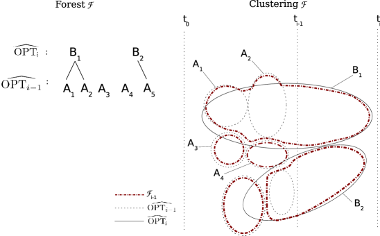
Figure 1. An example of a forest $\mathcal{F}$ given in left, and the corresponding clustering given in right. Here, we have $\text{$\widehat{\text{OPT}_{i}}$}=\{B_{1},B_{2}\}$ and $\text{$\widehat{\text{OPT}_{i-1}}$}=\{A_{1},\ldots,A_{5}\}$.

Let ${\mathcal{F}}_{i}$ be the forest obtained from ${\mathcal{F}}$ by erasing every node associated to clusters of $\widehat{\text{OPT}_{j}}$ for every $j<i$. With a slight abuse of notation, we define the following clustering ${\mathcal{F}}_{i}$ associated to that forest: there is one cluster $C$ for each tree of the forest defined as follows. For each node $A$ of the tree, let $k\geq i$ be such that $A\in\widehat{\text{OPT}_{k}}$: then $C$ contains $A\cap(t_{k-1},t_{k}]$ if $k>i$, and $C$ contains $A$ if $k=i$. This defines a sequence of clusterings such that ${\mathcal{F}}_{1}={\mathcal{F}}$ is the output of the algorithm, and ${\mathcal{F}}_{K}=\widehat{\text{OPT}_{K}}$.

Lemma 2.4 (Main lemma).

For any $2\leq i\leq K$,

$$\text{cost}({\mathcal{F}}_{i-1})-\text{cost}({\mathcal{F}}_{i})\leq\left((4+2\sqrt{3})\epsilon+\frac{\epsilon}{1-\epsilon}\right)t_{i}t_{K}.$$

We defer the proof of Lemma 2.4 to next section. Assuming Lemma 2.4, we upper-bound the cost of clustering $\mathcal{F}$.

Lemma 2.5 (Lemma 14, [2]).

For any $0<c<1$ and clustering $\mathcal{C}$, let $\mathcal{C}^{\prime}$ be the clustering obtained from $\mathcal{C}$ by splitting all clusters of $\mathcal{C}$ of size less than $cn$, where $n$ is the number of vertices. Then $\text{cost}(\mathcal{C}^{\prime})\leq\text{cost}(\mathcal{C})+cn^{2}/2$.

Lemma 2.6.

$\text{cost}(\mathcal{F})\leq((2\sqrt{3}+9/2)\epsilon+\frac{\epsilon}{1-\epsilon}+\epsilon^{4}/2)\frac{2\tau-1}{\tau-1}t_{K}^{2}$.

Proof 2.7.

We write: $\text{cost}(\mathcal{F})=\text{cost}(\widehat{\text{OPT}_{K}})+\sum_{i=2}^{K}(\text{cost}(\mathcal{F}_{i-1})-\text{cost}({\mathcal{F}}_{i}))$.By definition, $\widehat{\text{OPT}_{K}}$ contains the $1/\epsilon$ largest clusters of $\text{OPT}_{K}^{\prime}$. Then the remaining clusters of $\text{OPT}_{K}^{\prime}$ are of size at most $\epsilon t_{K}$. By Lemma 2.5, the cost of $\widehat{\text{OPT}_{K}}$ is at most $\text{cost}(\text{$\text{OPT}_{K}^{\prime}$})+\epsilon t_{K}^{2}/2\leq{(\alpha+\epsilon)t_{K}^{2}/2}$. Applying Lemma 2.4, and summing over $2\leq i\leq K$, we get

$$\text{cost}(\mathcal{F})\leq{(\alpha+\epsilon)t_{K}^{2}/2}+\left((4+2\sqrt{3})\epsilon+\frac{\epsilon}{1-\epsilon}\right)\sum_{i}{t_{i}}t_{K}.$$

By definition of the update times $(t_{i})_{i}$, for any $j>0$ there exists at most one $t_{i}$ such that $\tau^{j}\leq t_{i}<\tau^{j+1}$. Let $L$ be such that $\tau^{L}\leq t_{K}<\tau^{L+1}$. Then

$$\sum_{1\leq i\leq K}{t_{i}}\leq\sum_{1\leq i\leq K-1}{t_{i}}+t_{K}\leq\sum_{1\leq j\leq L}{\tau^{j}}+t_{K}\leq\frac{\tau^{L+1}}{\tau-1}+t_{K}\leq\frac{2\tau-1}{\tau-1}t_{K}.$$

Hence the desired bound on $\text{cost}(\mathcal{F})$.

Proof 2.8 (Proof of Theorem 4).

Fix an input graph of size $n$, such that $\text{profit}(\text{OPT})\geq(1-\alpha/2){n\choose 2}$. By Lemma 2.6, at time $t_{K}$, Algorithm 3 has clustering $\mathcal{F}$ with $\text{cost}(\mathcal{F})\leq O(\epsilon)\frac{2\tau-1}{\tau-1}t_{K}^{2}.$

By definition of the update times, $n<\tau t_{K}$. To guarantee a competitive ratio of $0.5+\eta$, for some $\eta$, the cost must not exceed $(0.5-\eta){n\choose 2}$ at time $n$, when all vertices $t_{K}+1,\ldots,n$ are added as singleton clusters. The number of new edges added to the graph between times $t_{K}$ and $n$ is ${n-t_{K}\choose 2}+t_{K}(n-t_{K})$. We must have

$$\frac{2\tau-1}{\tau-1}O(\epsilon)t_{K}^{2}+{n-t_{K}\choose 2}+t_{K}(n-t_{K})\leq(0.5-\eta){n\choose 2},$$ (2.2)

for some $0<\eta<0.5$. Using the fact that $n-t_{K}\leq(\tau-1)t_{K}$ and $t_{K}\leq n-1$, to satisfy (2.2), it suffices to have

$$\frac{2\tau-1}{\tau-1}O(\epsilon)t_{K}^{2}+t_{K}^{2}(\tau-1)^{2}/2+(\tau-1)t_{K}^{2}\leq(0.5-\eta)t_{K}^{2}/2,$$

which is equivalent to (2.1). Moreover we have the following natural constraints on constants $\eta$, $\epsilon$ and $\tau$: $0<\eta<0.5$, $0<\epsilon<1$, and $\tau>1$. Then, for any set of values of constants $\eta$, $\epsilon$, $\tau$ verifying those constraints, Algorithm Dense is $0.5+\eta$-competitive.

2.3.3. The core of the analysis: proof of Lemma 2.4

Lemma 2.9.

Let $\mathcal{S}^{i}$ be the set of vertices of the non-singleton clusters that are not among the $1/\epsilon^{2}-1/\epsilon$ largest clusters of $\widehat{\text{OPT}_{i-1}}$. Then $|\mathcal{S}^{i}|\leq\frac{\epsilon}{1-\epsilon}t_{i-1}.$

Proof 2.10.

Let $C$ be a cluster of $\widehat{\text{OPT}_{i-1}}$, such that $C\subseteq\mathcal{S}^{i}$. Then ${|C|\leq(1/\epsilon^{2}-1/\epsilon)^{-1}t_{i-1}}$. Since there are at most $1/\epsilon$ such clusters, the number of vertices of these are at most $1/\epsilon(1/\epsilon^{2}-1/\epsilon)^{-1}t_{i-1}$.

Notation 5.

For any $i\neq j$, and a cluster $B$ of $\text{OPT}_{i}^{\prime}$, we denote by $\gamma^{i,j}_{B}$ the square root of the number of edges of $[1,t_{\min(i,j)}]\times[1,t_{\min(i,j)}]$, adjacent to at least one node of $B$, and which are classified differently in $\text{OPT}_{i}^{\prime}$ and in $\text{OPT}_{j}^{\prime}$.

We refer to non singleton clusters as large clusters.

Lemma 2.11.

Let $\mathcal{T}^{i}$ be the set of vertices of those $1/\epsilon^{2}-1/\epsilon$ largest clusters of $\widehat{\text{OPT}_{i-1}}$ that are not half-contained in any cluster of $\text{OPT}_{i}^{\prime}$. Then $|\mathcal{T}^{i}|\leq\sqrt{6}\sum_{\text{large }C\in\text{$\widehat{\text{OPT}_{i-1}}$}}{\gamma^{i,i-1}_{C}}$.

Let $B$ be a cluster of $\widehat{\text{OPT}_{i}}$. For any $j\leq i$, we define $\mathcal{C}_{j}(B)$ as the cluster associated with the tree of $\mathcal{F}_{j}$ that contains $B$. For any $B\in\text{$\widehat{\text{OPT}_{i}}$}$, we call $\mathcal{C}_{i-1}(B)$ the extension of $\mathcal{C}_{i}(B)$ to $\mathcal{F}_{i-1}$. By definition of $\mathcal{F}_{i}$, the following lemma is easy.

Lemma 2.12.

For any $B\in\text{$\widehat{\text{OPT}_{i}}$}$, the restriction of $\mathcal{C}_{i-1}(B)$ to $(t_{i-1},t_{K}]$ is equal to the restriction of $\mathcal{C}_{i}(B)$ to $(t_{i-1},t_{K}]$.

Let $(A_{j})_{j}$ denote the clusters of $\widehat{\text{OPT}_{i-1}}$ that are half-contained in $B$. We define $\delta^{i}(B)$ as the symmetric difference of the restriction of $B$ to $[1,t_{i-1}]$ and $\cup_{j}{A_{j}}$:

$$\delta^{i}(B)=(B\cap[1,t_{i-1}])\Delta\cup_{j}{A_{j}}.$$

Lemma 2.13.

For any cluster $C_{i}$ of $\mathcal{F}_{i}$, let $C_{i}^{\prime}$ denote the extension of $C_{i}$ to $\mathcal{F}_{i-1}$. Then

$$\bigcup_{C_{i}\in\mathcal{F}_{i}}{{C}_{i}\setminus{C}_{i}^{\prime}}\subseteq\mathcal{S}^{i}\cup\mathcal{T}^{i}\cup\bigcup_{\text{large }B\in\text{$\widehat{\text{OPT}_{i}}$}}{\delta^{i}(B)}$$

Proof 2.14.

By Lemma 2.12, the partition of the vertices $(t_{i-1},t_{K}]$ is the same for $C_{i}$ as for $C_{i}^{\prime}$. So $C_{i}$ and $C_{i}^{\prime}$ only differ in the vertices of $[1,t_{i-1})$:

$$\bigcup_{C_{i}\in\mathcal{F}_{i}}{{C}_{i}\setminus{C}_{i}^{\prime}}\subseteq\bigcup_{B\in\text{$\widehat{\text{OPT}_{i}}$}}{\delta^{i}(B)}.$$

We will show that for a singleton cluster $B$ of $\widehat{\text{OPT}_{i}}$, $\delta^{i}(B)$ is included in $\mathcal{S}^{i}\cup\mathcal{T}^{i}\bigcup_{\text{large }B\in\text{$\widehat{\text{OPT}_{i}}$}}{\delta^{i}(B)}$, which yields the lemma.

Let $B=\{v\}$ be a singleton cluster of $\widehat{\text{OPT}_{i}}$ such that $\delta^{i}(B)\neq\{\}$. A non-singleton cluster cannot be half-contained in a singleton cluster so we conclude no clusters are half-contained in $B$ and hence $\delta^{i}(B)=\{v\}$. By definition of $\delta^{i}(B)$, $v\in[1,t_{i-1}]$. So there exists a cluster $A$ of $\widehat{\text{OPT}_{i-1}}$ that contains $v$. Clearly $A$ is not a singleton since otherwise $\delta^{i}(B)$ would be $\{\}$. There are two cases.

First, if $A$ is half-contained in a cluster $B^{\prime}\neq B$ of $\widehat{\text{OPT}_{i}}$ then cluster $B^{\prime}$ is necessarily large since it contains more than one vertex of $A$. Then we have $v\in\delta^{i}(B^{\prime})$.

Second, if $A$ is not half-contained in any cluster of $\widehat{\text{OPT}_{i}}$ then $A\subseteq\mathcal{S}^{i}\cup\mathcal{T}^{i}$. In fact, if $A$ is half-contained in a cluster of $\text{OPT}_{i}^{\prime}$ which is split into singletons in $\widehat{\text{OPT}_{i}}$, then $A$ is not one of the $1/\epsilon^{2}-1/\epsilon$ largest clusters of $\widehat{\text{OPT}_{i-1}}$, and $A\subseteq\mathcal{S}^{i}$. If $A$ is not half-contained in any cluster of $\text{OPT}_{i}^{\prime}$, then $A\subseteq\mathcal{T}^{i}$ if $A$ is one of the $1/\epsilon^{2}-1/\epsilon$ largest clusters of $\widehat{\text{OPT}_{i-1}}$ and $A\subseteq\mathcal{S}^{i}$ otherwise.

Lemma 2.15.

For any large cluster $B$ of $\widehat{\text{OPT}_{i}}$, $|\delta^{i}(B)|\leq 2\sqrt{2}\gamma^{i,i-1}_{B}$.

Proof 2.16.

Let $B^{\prime}$ denote the restriction of $B$ to $[1,t_{i-1}]$. We first show that

$$1/2(|\cup_{j}{A_{j}}\setminus B^{\prime}|)^{2}\leq(\gamma^{i,i-1}_{B})^{2}.$$

Observe that $(\gamma^{i,i-1}_{B})^{2}$ includes all edges $uv$ such that one of the following two cases occurs.

First, if $u\in A_{j}\setminus B$ and $v\in A_{j}\cap B$: such edges are internal in the clustering $\text{OPT}_{i-1}^{\prime}$ but external in the clustering $\text{OPT}_{i}^{\prime}$. The number of edges of this type is $\sum_{j}|A_{j}\setminus B|\cdot|A_{j}\cap B|$. Since $A_{j}$ is half-contained in $B$, this is at least $\sum_{j}|A_{j}\setminus B|^{2}$.

Second, if $u\in A_{j}\cap B$ and $v\in A_{k}\cap B$ with $j\neq k$: such edges are external in the clustering $\text{OPT}_{i-1}^{\prime}$ but internal in the clustering $\text{OPT}_{i}^{\prime}$. The number of edges of this type is $\sum_{j<k}|A_{j}\cap B|\cdot|A_{k}\cap B|\geq\sum_{j<k}|A_{j}\setminus B|\cdot|A_{k}\setminus B|$.

Summing, it is easy to infer that $(\gamma^{i,i-1}_{B})^{2}\geq(1/2)\left(\sum_{j}|A_{j}\setminus B|\right)^{2}=(1/2)|\cup_{j}A_{j}\setminus B^{\prime}|^{2}$. Let $(A^{\prime}_{j})_{j}$ denote the clusters of $\widehat{\text{OPT}_{i-1}}$ that are not half-contained in $B$, but have non-empty intersections with $B$. We now show that

$$1/2(|B^{\prime}\setminus\cup_{j}{A^{\prime}_{j}}|)^{2}\leq(\gamma^{i,i-1}_{B})^{2}.$$

We have $B^{\prime}\setminus\cup_{j}{A_{j}}=\cup_{j}{(A^{\prime}_{j}\cap B)}$. Observe that any $A^{\prime}_{j}$ is a large cluster of $\widehat{\text{OPT}_{i-1}}$, thus a cluster of $\text{OPT}_{i-1}^{\prime}$. Then $(\gamma^{i,i-1}_{B})^{2}$ includes all edges $uv$ such that one of the following two cases occurs

First, if $u\in A^{\prime}_{j}\setminus B$ and $v\in A^{\prime}_{j}\cap B$: such edges are internal in the clustering $\text{OPT}_{i-1}^{\prime}$ but external in the clustering $\text{OPT}_{i}^{\prime}$. The number of edges of this type is $\sum_{j}|A^{\prime}_{j}\setminus B|\cdot|A^{\prime}_{j}\cap B|$. Since $A^{\prime}_{j}$ is not half-contained in $B$, this is at least $\sum_{j}|A^{\prime}_{j}\cap B|^{2}$.

Second, if $u\in A^{\prime}_{j}\cap B$ and $v\in A^{\prime}_{k}\cap B$ with $j\neq k$: such edges are external in the clustering $\text{OPT}_{i-1}^{\prime}$ but internal in the clustering $\text{OPT}_{i}^{\prime}$. The number of edges of this type is $\sum_{j<k}|A^{\prime}_{j}\cap B|\cdot|A^{\prime}_{k}\cap B|$.

Summing, we get

$$(\gamma^{i,i-1}_{B})^{2}\geq(1/2)\left(\sum_{j}|A^{\prime}_{j}\cap B|\right)^{2}=(1/2)|B^{\prime}\setminus\cup_{j}A^{\prime}_{j}|^{2}.$$

Lemma 2.17.

For any $i\geq 1$, $\widehat{\text{OPT}_{i}}$ has at most $1/\epsilon^{2}$ non singleton clusters, all of which are clusters of $\text{OPT}_{i}^{\prime}$

Proof 2.18.

By definition, $\widehat{\text{OPT}_{1}}$ has at most $1/\epsilon^{2}$ non singleton clusters. For any $i>1$, a cluster of $\widehat{\text{OPT}_{i-1}}$ can only be half-contained in one cluster of $\text{OPT}_{i}^{\prime}$. Therefore given $\widehat{\text{OPT}_{i-1}}$, at most $1/\epsilon^{2}$ clusters of $\text{OPT}_{i}^{\prime}$ are marked. Thus $\widehat{\text{OPT}_{i}}$ has at most $1/\epsilon^{2}$ clusters.

We can now prove Lemma 2.4.

Proof 2.19 (Proof of Lemma 2.4).

By Lemma 2.12, clusterings $\mathcal{F}_{i}$ and $\mathcal{F}_{i-1}$ only differ in their partition of $[1,t_{i-1}]$. Then the set of the vertices that are classified differently in $\mathcal{F}_{i}$ and $\mathcal{F}_{i-1}$ is $\cup_{i}C_{i}\setminus C_{i-1}$. Each of these vertices creates at most $t_{K}$ disagreements:

$$\begin{split}\text{cost}({\mathcal{F}}_{i-1})-\text{cost}({\mathcal{F}}_{i})&\leq\sum_{C_{i}\in\mathcal{F}_{i}}{|C_{i}\setminus C_{i-1}|}t_{K}\\ \end{split}$$ (2.3)

By Lemmas 2.13 and 2.15,

$$\sum_{C_{i}\in\mathcal{F}_{i}}{|C_{i}\setminus C_{i-1}|}t_{K}\leq\left(2\sqrt{2}\Bigg{(}\sum_{\text{large }B\in\widehat{\text{OPT}_{i}}}\gamma^{i,i-1}_{B}\Bigg{)}+|\mathcal{S}^{i}|+|\mathcal{T}^{i}|\right)t_{K}.$$ (2.4)

By Lemmas 2.9 and 2.11,

$$|\mathcal{S}^{i}|\leq\frac{\epsilon}{1-\epsilon}t_{i-1}\hbox{ and }|\mathcal{T}^{i}|\leq\sqrt{6}\sum_{\text{large }B\in\text{$\widehat{\text{OPT}_{i-1}}$}}{\gamma^{i-1,i}_{B}}$$ (2.5)

The term $\sum_{\text{large }B\in\widehat{\text{OPT}_{i-1}}}\gamma^{i-1,i}_{B}$ can be seen as the $\ell_{1}$ norm of the vector $(\gamma^{i-1,i}_{B})_{\text{large }B}$. Since $\widehat{\text{OPT}_{i-1}}$ has at most $1/\epsilon^{2}$ large clusters by Lemma 2.17, we can use Hölder’s inequality:

$$\begin{split}\sum_{\text{large }B\in\widehat{\text{OPT}_{i-1}}}\gamma^{i-1,i}_{B}&=\|(\gamma^{i-1,i}_{B})_{\text{large }B}\|_{1}\leq 1/\epsilon\|(\gamma^{i-1,i}_{B})_{\text{large }B}\|_{2}.\end{split}$$

By definition we have $\|(\gamma^{i-1,i}_{B})_{\text{large B}}\|_{2}\leq\sqrt{2(\text{cost}(\text{$\text{OPT}_{i-1}^{\prime}$})+\text{cost}(\text{$\text{OPT}_{i}^{\prime}$}))}$. Thus

$$\sum_{\text{large }B\in\widehat{\text{OPT}_{i-1}}}\gamma^{i-1,i}_{B}\leq 1/\epsilon\sqrt{2(\alpha t_{i-1}^{2}/2+\alpha t_{i}^{2}/2)}\leq\frac{\sqrt{2\alpha}}{\epsilon}t_{i}.$$ (2.6)

Similarly, we have

$$\sum_{\text{large }B\in\text{$\widehat{\text{OPT}_{i}}$}}{\gamma^{i,i-1}_{B}}\leq\frac{\sqrt{2\alpha}}{\epsilon}t_{i}.$$ (2.7)

Combining equations (2.3) through (2.7) and $\alpha=\epsilon^{4}$ yields

$$\text{cost}({\mathcal{F}}_{i-1})-\text{cost}({\mathcal{F}}_{i})\leq\left((4+2\sqrt{3})\epsilon+\frac{\epsilon}{1-\epsilon}\right)t_{i}t_{K}$$

3. Minimizing Disagreements Online

Theorem 6.

Algorithm Greedy is $(2n+1)$-competitive for MinDisAgree.

To prove Theorem 6, we need to compare the cost of the optimal clustering to the cost of the clustering constructed by the algorithm. The following lemma reduces this to, roughly, analyzing the number of vertices classified differently.

Lemma 3.1.

Let $\mathcal{W}$ and $\mathcal{W}^{\prime}$ be two clusterings such that there is an injection $W^{\prime}_{i}\in\mathcal{W}^{\prime}\rightarrow W_{i}\in\mathcal{W}$. Then $\text{cost}(\mathcal{W}^{\prime})-\text{cost}(\mathcal{W})\leq n\sum_{i}|W_{i}^{\prime}\setminus W_{i}|$.

For subsets of vertices $S_{1},\ldots,S_{m}$, we will write, with a slight abuse of notation, $\Gamma^{+}(S_{1},\ldots,S_{m})$ for the set of edges in $\Gamma^{+}(S_{i},S_{j})$ for any $i\neq j$: $\Gamma^{+}(S_{1},\ldots,S_{m})=\cup_{i\neq j}{\Gamma^{+}(S_{i},S_{j})}$.

Lemma 3.2.

Let $C$ be a cluster created by Greedy, and $\mathcal{W}=\{W_{1},\ldots,W_{K}\}$ denote the clusters of OPT. Then $|C|\leq\max_{i}|C\cap W_{i}|+2|\Gamma^{+}(C\cap W_{1},\ldots,C\cap W_{K})|.$. We call $\displaystyle i_{0}=\arg\max_{i}|C\cap W_{i}|$ the leader of $C$.

Proof 3.3 (Proof of Theorem 6).

Let $\mathcal{C}$ denote the clustering given by Greedy. For every cluster $W_{i}$ of OPT, merge all the clusters of $\mathcal{C}$ that have $i$ as their leaders. Let $\mathcal{C}^{\prime}=(W^{\prime}_{i})$ be this new clustering. By definition of the greedy algorithm, this operation can only increase the cost since every pair of clusters have a negative-majority cut at the end of the algorithm:$\text{cost}(\mathcal{C})\leq\text{cost}(\mathcal{C}^{\prime}).$ We apply Lemma 3.1 to $\mathcal{W}=$OPT and $\mathcal{W^{\prime}}=\mathcal{C}^{\prime}$, and obtain: $\text{cost}(\mathcal{C}^{\prime})\leq\text{cost}(\text{OPT})+n\sum_{i}|W_{i}^{\prime}\setminus W_{i}|$. By definition of $\mathcal{C}^{\prime}$ we have $|W_{i}^{\prime}\setminus W_{i}|=\sum_{\begin{subarray}{c}C\in\mathcal{C}:\text{leader}(C)=i\end{subarray}}\sum_{j\neq i}{|C\cap W_{j}|},$ hence

$$\sum_{i}|W_{i}^{\prime}\setminus W_{i}|=\sum_{C\in\mathcal{C}}\sum_{j\neq\text{leader}(C)}{|C\cap W_{j}|}.$$

By Lemma 3.2, $\sum_{j\neq\text{leader}(C)}{|C\cap W_{j}|}\leq 2|\Gamma^{+}(C\cap W_{1},\ldots,C\cap W_{K})|$. Finally, to bound OPT from below, we observe that, for any two clusterings $\mathcal{C}$ and $\mathcal{W}$, it holds that the sum over $C\in\mathcal{C}$ of ${|\Gamma^{+}(C\cap W_{1},\ldots,C\cap W_{K})|}$ is less than $\text{cost}(\mathcal{W})$. Combining these inequalities yields the theorem.

Theorem 7.

Let ALG be a randomized algorithm for MinDisAgree. Then there exists an instance on which ALG has cost at least $n-1-\text{cost}(\text{OPT})$ where OPT is the offline optimum. If OPT is constant then $\text{cost}(\text{ALG})=\Omega(n)\text{cost}(\text{OPT})$.

Proof 3.4.

Consider two cliques $A$ and $B$, each of size $m$, where all the internal edges of $A$ and $B$ are positive. Choose a vertex $a$ in $A$, and a set of vertices $b_{1},\ldots,b_{k}$ in $B$. Define the edge labels of $ab_{i}$ as positive, for all $1\leq i\leq k$ and the rest of the edges between $A$ and $B$ as negative. Define an input sequence starting with $a,b_{1},\ldots,b_{k}$, followed by the rest of the vertices in any order.

References

• [1] Nir Ailon, Moses Charikar, and Alantha Newman. Aggregating inconsistent information: ranking and clustering. In STOC ’05: Proceedings of the thirty-seventh annual ACM symposium on Theory of computing, pages 684–693, New York, NY, USA, 2005. ACM Press.
• [2] Nikhil Bansal, Avrim Blum, and Shuchi Chawla. Correlation clustering. Mach. Learn., 56(1-3):89–113, 2004.
• [3] Amir Ben-Dor, Ron Shamir, and Zohar Yakhini. Clustering gene expression patterns. Journal of Computational Biology, 6(3-4):281–297, 1999.
• [4] Allan Borodin and Ran El-Yaniv. Online computation and competitive analysis. Cambridge University Press, New York, NY, USA, 1998.
• [5] Moses Charikar, Chandra Chekuri, Tomas Feder, and Rajeev Motwani. Incremental clustering and dynamic information retrieval. SIAM J. Comput., 33(6):1417–1440, 2004.
• [6] Moses Charikar, Venkatesan Guruswami, and Anthony Wirth. Clustering with qualitative information. In focs, volume 00, page 524, Los Alamitos, CA, USA, 2003. IEEE Computer Society.
• [7] Moses Charikar, Venkatesan Guruswami, and Anthony Wirth. Clustering with qualitative information. J. Comput. Syst. Sci., 71(3):360–383, 2005.
• [8] William W. Cohen and Jacob Richman. Learning to match and cluster large high-dimensional data sets for data integration. In KDD ’02: Proceedings of the eighth ACM SIGKDD international conference on Knowledge discovery and data mining, pages 475–480, New York, NY, USA, 2002. ACM.
• [9] Erik D. Demaine, Dotan Emanuel, Amos Fiat, and Nicole Immorlica. Correlation clustering in general weighted graphs. Theor. Comput. Sci., 361(2):172–187, 2006.
• [10] Jenny Rose Finkel and Christopher D. Manning. Enforcing transitivity in coreference resolution. In Proceedings of ACL-08: HLT, Short Papers, pages 45–48, Columbus, Ohio, June 2008. Association for Computational Linguistics.
• [11] Ioannis Giotis and Venkatesan Guruswami. Correlation clustering with a fixed number of clusters. Theory of Computing, 2(1):249–266, 2006.
• [12] Thorsten Joachims and John Hopcroft. Error bounds for correlation clustering. In ICML ’05: Proceedings of the 22nd international conference on Machine learning, pages 385–392, New York, NY, USA, 2005. ACM.
• [13] Marek Karpinski and Warren Schudy. Linear time approximation schemes for the Gale-Berlekamp game and related minimization problems. In STOC ’09: Proceedings of the 41st annual ACM symposium on Theory of computing, pages 313–322, 2009.
• [14] Claire Mathieu and Warren Schudy. Correlation clustering with noisy input. In To appear in Procs. 21st SODA, preprint: http://www.cs.brown.edu/$\sim$ws/papers/cluster.pdf, 2010.
• [15] Ron Shamir, Roded Sharan, and Dekel Tsur. Cluster graph modification problems. Discrete Appl. Math., 144(1-2):173–182, 2004.