Correlation Properties of anisotropic XY Model with a Sudden Quench

Abstract

Starting from a general Hamiltonian which may undergo a quantum phase transition (QPT) with the change of a controllable parameter, we obtain a general conclusion that in a sudden quench system, when the final Hamiltonian is fixed, the behavior of the time-averaged expectation of any observable has close relationship with the gapless excitation of the initial Hamiltonian. To clarify our conclusion, we investigate the two-spin correlation of a XY chain in a transverse field under a sudden quench at zero temperature. The critical property of the derivative of quench two-spin correlation and the long-range correlation of the quench system are analyzed.

I Introduction

Quantum phase transition (QPT), which is driven by quantum fluctuation and occurs at zero temperature, is a very important research area recently book . Besides the static properties of QPT, the non-equilibrium dynamics induced by the quench of the parameter in the Hamiltonian through a critical point has always been an attractive topic in condensed matter physics Na41951 ; PRA69053616 ; PRL95105701 ; PRL95245701 ; PRB72161201 ; PRA72052319 ; PRA73063405 ; PRB76174303 ; PRA75023603 ; PRL100077204 ; Np4 477 ; nature452 ; PRB80054404 ; PRL98050405 ; PRL102245701 ; nature449324 ; PRA79021608 .

Generally speaking, a dynamical evolution can be induced by either a sudden quench or a slow quench. Taking the spin chain in the magnetic field as an example, the typical paradigm of sudden quench is as follows. Initially ($t<0$) the magnetic field $h(t<0)=a$. Then at time $t=0$ the magnetic field is changed to $b$ suddenly, namely $h(t\geq 0)=b$ and the system begins to evolve from the initial state. After a long enough time evolution, the time-averaged expectation value of an observable $A$ reaches a steady value, which we define as quench $A$. Quench $A$ is $\langle A(a,b)\rangle=\lim_{t\rightarrow\infty}\frac{1}{t}\int_{0}^{t}\langle A(a,b,\tau)\rangle d\tau$ nature452 , with $\langle A(a,b,\tau)\rangle$ the expectation value of observable $A$ at time $t=\tau$ with initial magnetic field $a$ and final magnetic field $b$. One can fix $b$($a$) to investigate the relation between quench $A$ and $a$($b$).

The magnetization $M$ and its derivative with respect to magnetic field $\partial_{h}M$ of transverse Ising model are analyzed in Ref. PRB80054404 . It is found that $\partial_{h}M$ has similar behavior for static system and sudden quench system. Here interesting questions arise: why does this similarity happen and whether other quantities still exhibit such similarity?

In this work, we start from a general Hamiltonian $H(\lambda)$ containing a controllable parameter $\lambda$ to search for the answers. We obtain a general conclusion that in a sudden quench system, when the final Hamiltonian is fixed, the behavior of the time-averaged expectation of any observable has close relationship with the gapless excitation of the initial Hamiltonian. There is a similarity between the critical phenomena of sudden quench and static system. Then we numerically investigate the sudden quench properties of two-spin correlation of an anisotropic XY chain in a transverse field PRA21075 . The results are consistent with our conclusion. We also research the long-range correlation of the system in both directions parallel and perpendicular to the magnetic field. There is no qualitative difference between static and sudden quench case in the direction parallel to the magnetic field, but a remarkable difference exists in the direction perpendicular to the magnetic field, which is consistent with the result in Ref.PRA69053616 . At last, we briefly discuss the case in which initial Hamiltonian is fixed.

II General Model

Here we consider a general Hamiltonian $H(\lambda)=H_{0}+\lambda H_{I}$ which contains a controllable parameter $\lambda$. We suppose the ground state of $H(\lambda)$ is non-degenerate and with the varying of $\lambda$ the system can undergo a QPT happening at $\lambda=\lambda_{c}$, where the energy gap of $H(\lambda)$ vanishes in the thermodynamics limit (TL). This is the case for many condensed matter systems, especially for spin chains. For example $H_{I}=\sum_{i}\sigma_{i}^{z}$ and $\lambda$ is the magnetic field for transverse Ising model.

Now we try to derive the singular behavior of the time-averaged expectation value of any observable $A$ when QPT happens, both for static case and sudden quench case. At time $t<0$, $\lambda=a$ and the eigenvectors and eigenvalues of $H(a)$ are denoted as $|\psi_{n}(a)\rangle$ and $E_{n}(a)$ respectively. At zero temperature the system is in the ground state of this initial Hamiltonian $H(a)$, namely $|\Psi(t<0)\rangle=|\psi_{0}(a)\rangle$. Therefore for static case, which means $\lambda=a$ for $t\geq 0$, the the time-averaged expectation value is just $\langle A(a)\rangle=\langle\psi_{0}(a)|A|\psi_{0}(a)\rangle$. By the perturbation theory, we know

$$|\psi_{0}(a+\delta a)\rangle=|\psi_{0}(a)\rangle+\delta a\sum_{m\neq 0}\frac{(H_{I})_{m0}}{E_{0}(a)-E_{m}(a)}|\psi_{m}(a)\rangle$$

with $(H_{I})_{m0}=\langle\psi_{m}(a)|H_{I}|\psi_{0}(a)\rangle$, so

$$\partial_{a}|\psi_{0}(a)\rangle=\sum_{m\neq 0}\frac{(H_{I})_{m0}}{E_{0}(a)-E_{m}(a)}|\psi_{m}(a)\rangle,$$

which leads to

$$\partial_{a}\langle A(a)\rangle=2\sum_{m\neq 0}\frac{\Re[(H_{I})_{0m}\langle\psi_{m}(a)|A|\psi_{0}(a)\rangle]}{E_{0}(a)-E_{m}(a)}$$ (1)

straightforwardly, where $\Re(z)$ means the real part of a complex number $z$. One can expect that $\partial_{a}\langle A(a)\rangle$ will behave singularly at $a=\lambda_{c}$ because the energy gap vanishes in TL.

If at time $t=0$, $\lambda$ is suddenly changed to $b$ and $\lambda=b$ is kept for $t>0$, the system will evolve under sudden quench. The eigenvectors and eigenvalues of the final Hamiltonian $H(b)$ are denoted as $|\phi_{n}(b)\rangle$ and $\omega_{n}$ respectively. The time-evolving wave function of the system at $t>0$ is $|\Psi(t>0)\rangle=\sum_{n}\langle\phi_{n}(b)|\psi_{0}(a)\rangle e^{-i\omega_{n}t}|\phi_{n}(b)\rangle$, where we omit the relative phase. The time-averaged expectation value is

$$\langle A(a,b)\rangle = \lim_{t\rightarrow\infty}\frac{1}{t}\int_{0}^{t}\langle A(a,b,\tau)\rangle d\tau$$

$$= \sum_{n}\langle\psi_{0}(a)|\phi_{n}(b)\rangle\langle\phi_{n}(b)|\psi_{0}(a)\rangle\langle\phi_{n}(b)|A|\phi_{n}(b)\rangle.$$

So we have

$$\partial_{a}\langle A(a,b)\rangle = 2\sum_{m\neq 0}\sum_{n}\frac{\langle\phi_{n}(b)|A|\phi_{n}(b)\rangle}{E_{0}(a)-E_{m}(a)}\times\Re[(H_{I})_{0m}\langle\psi_{m}(a)|\phi_{n}(b)\rangle\langle\phi_{n}(b)|\psi_{0}(a)\rangle].$$ (2)

When $b\neq\lambda_{c}$, the numerator in the above Eq.(2) is not zero. Therefore $\partial_{a}\langle A(a,b)\rangle$ will show singularity at $a=\lambda_{c}$ because of the vanishing of the energy gap in TL. However if $b=\lambda_{c}=a$, we have $\psi=\phi$, so in Eq.(2) $\langle\psi_{m}(a)|\phi_{n}(b)\rangle\langle\phi_{n}(b)|\psi_{0}(a)\rangle=\delta_{m,n}\delta_{n,0}$. Considering $m\neq 0$ in the sum, we can see both the numerator and denominator in Eq.(2) are zero at $a=b=\lambda_{c}$, meaning that $\partial_{a}\langle A(a,\lambda_{c})\rangle$ maybe has no singular behavior at $a=\lambda_{c}$.

Because Eqs.(1) and (2) share the same denominator, we conclude that there must be similarity between the critical singular behaviors of $\partial_{a}\langle A(a)\rangle$ and $\partial_{a}\langle A(a,b)\rangle$. The singularity and scaling behaviors come from the vanishing of the energy gap of the initial Hamiltonian in TL. If there is a critical phenomenon of the initial Hamiltonian with a vanishing energy gap which can be indicated by the singular behavior of $\partial_{a}\langle A(a)\rangle$ at $a=\lambda_{c}$, $\partial_{a}\langle A(a,b)\rangle$ will also have a similar singular behavior at $a=\lambda_{c}$ if $b\neq\lambda_{c}$.

III XY spin chain model

In this paper, we use the anisotropic XY model in a transverse field under a sudden quench at zero temperature to check our conclusion in the above section. The Hamiltonian of the spin-1/2 anisotropic XY spin chain is

$$H=\sum_{j=0}^{N-1}\Big{\{}\frac{J}{2}\Big{[}(1+\gamma)\sigma_{j}^{x}\sigma_{j+1}^{x}+(1-\gamma)\sigma_{j}^{y}\sigma_{j+1}^{y}\Big{]}-h(t)\sigma_{j}^{z}\Big{\}},$$

where $J$ is the coupling constant, $\sigma_{j}^{x},\sigma_{j}^{y},\sigma_{j}^{z}$ are the Pauli operators at the $j$th lattice site and $J(1\pm\gamma)/2$ is the measure of the interaction strength in $x(y)$ component between two nearest-neighbor spins. $\gamma$ is the anisotropy parameter which can change from $0$ (XX model) to $1$ (Ising model). $h(t)$ is the time-dependent magnetic field. In our paper, we set $J=1>0$ for convenience and the periodic boundary condition $\sigma_{N}^{\alpha}=\sigma_{0}^{\alpha},\alpha=x,y,z$ is used. The phase diagram of this model is easy to be obtained. There are two kinds of phase transition in anisotropic XY spin chain model. One belongs to the universality class of the Ising phase transition and the other is anisotropic transition PRB76174303 . In this paper we focus on the Ising phase transition. The equilibrium Ising phase critical points are $|h|=1$. In $J=1>0$ case, the system has anti-ferromagnetic interaction with the staggered magnetization in the $x$ direction $\langle\sigma^{x}\rangle_{\textrm{stag}}=\frac{1}{N}\sum_{i=0}^{N-1}(-1)^{i}\langle\sigma_{i}^{x}\rangle$ as the order parameter. For $|h|<1$, the system is in an ordered phase with $|\langle\sigma^{x}\rangle_{\textrm{stag}}|=1$, while for $|h|>1$, the system is in a disordered phase with $\langle\sigma^{x}\rangle_{\textrm{stag}}=0$. Now we turn to the problem of dynamics under sudden quench. Using successive Jordan-Wigner, Fourier, and Bogoliubov transformations, the exact solutions of the evolved state of XY model under a sudden quench can be obtained PRA21075 , by which the quench dynamical properties of many observables such as magnetization and two-spin correlation can be studied. In our work we focus on the quench two-spin correlation, which is defined as $G^{\alpha}_{n}(a,b)=\lim_{t\rightarrow\infty}\frac{1}{t}\int_{0}^{t}\langle\sigma^{\alpha}_{0}(a,b,\tau)\sigma^{\alpha}_{n}(a,b,\tau)\rangle d\tau$, where $\alpha=x,y,z$, $n$ is the distance between two spins and $a$ ($b$) is the initial (final) magnetic field.

IV Quench two-spin correlation

As the beginning we want to clarify our conclusion in Sec.II by considering $\partial_{a}G^{z(x)}_{1}(a,b)$, namely the nearest-neighbor two-spin correlation. Due to the difficulty in the analytical calculation of them, we choose to numerically solve them. We let $\gamma=1$ for convenience in this part and one should note that all conclusions below are also valid for $\gamma\neq 1$.

In Fig.1(a), $\partial_{a}G^{z}_{1}(a,b\neq 1)$ diverges at $a=1$ for both the static and dynamical case. Moreover, we calculate that $\partial_{a}G^{z}_{1}(a,b)=\textrm{const}\times|a-1|^{-\mu}$ with $\mu\approx 0.25$, a universal exponent irrelevant with $b$ (Fig.1(b)). While as predicted in Sec.II, the sudden quench case with $b=1$ is very special. We can see from Fig.1(a) that $\partial_{a}G^{z}_{1}(a,1)$ is not divergent at $a=1$.

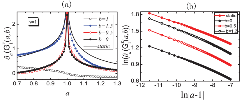
Figure 1: $\gamma=1$. (a) $\partial_{a}G^{z}_{1}(a,b)$ for static case and dynamical cases $b=0,0.5,1,1.5$. (b) $\ln(\partial_{a}G^{z}_{1}(a,b))$ as a function of $\ln|a-1|$. One can see the slopes of the lines for different $b$ are all the same, namely a universal constant -0.25.

Similar to $G_{1}^{z}(a,b)$, $\partial_{a}G^{x}_{1}(a,b\neq 1)$ diverges at $a=1$ for static and sudden quench case. After numerical analysis, we can find $\partial_{a}G^{x}_{1}(a,b)=\frac{1}{\pi}\ln|a-1|+f(b)$, with $f(b)$ a constant which we do not concern with (Fig.2(b)). We also can see from Fig.2(a) that $\partial_{a}G^{x}_{1}(a,1)$ is not divergent at $a=1$.

Through the comparison between static and sudden quench cases of XY model, we find that in general sudden quench case ($b\neq 1$), the quench system and static system share similar critical scaling form of $\partial_{a}G^{z(x)}_{1}(a,b)$. This is consistent with our conclusion in Sec.II and reflects the memory of the quench system to the initial Hamiltonian.

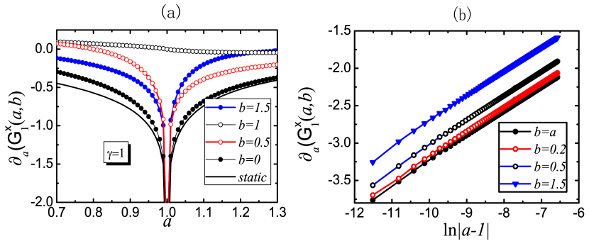
Figure 2: $\gamma=1$. (a) $\partial_{a}G^{x}_{1}(a,b)$ for static case and dynamical cases $b=0,0.5,1,1.5$. (b) $\partial_{a}G^{x}_{1}(a,b)$ as a function of $\ln|a-1|$. One can see the slopes of the lines for different $b$ are all the same, namely a universal constant $1/\pi$.

Now we shift our focus from the nearest-neighbor two-spin correlation to the correlation between two spins with arbitrary distance $n$. We show $G^{z}_{n}(a,b)$ as a function of $a$ and $n$ for both static and sudden quench case in Fig.3, where $\gamma=0.6$ is used. From this figure, we know as $n$ increases, $G^{z}_{n}(a,b)$ reaches a constant quickly after a little increase of $n$. There is no qualitative difference between static and general dynamical case.

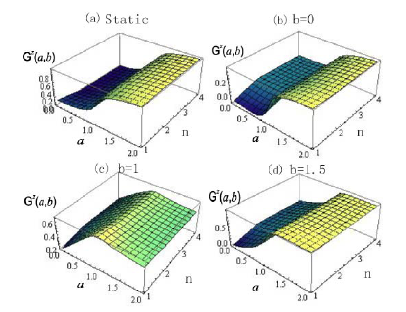
Figure 3: $\gamma=0.6$. $G^{z}_{n}(a,b)$ for (a) The static case $b=a$, (b) $b=0$, (c) $b=1$ and (d) $b=1.5$.

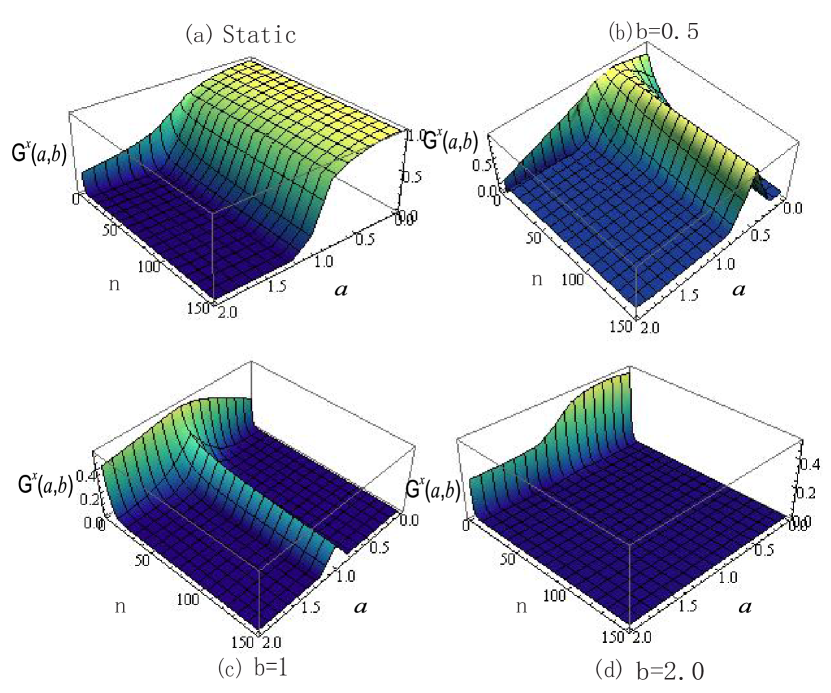
Figure 4: $\gamma=1$. $G^{x}_{n}(a,b)$ in (a) static system and dynamical systems with (b) $b=0.5$, (c) $b=1$ and (d) $b=2$.

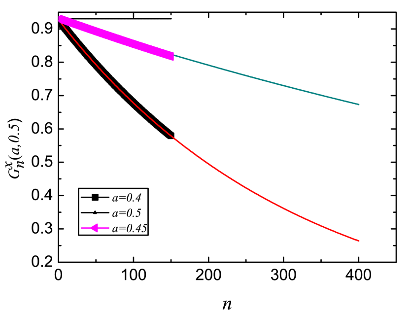
Figure 5: Numerical fitting of $G_{n}^{x}(a,b)$ at $b=0.5$ up to $n=150$. Through numerical fit of the two typical data $G^{x}_{n}(0.4,0.5)$ and $G^{x}_{n}(0.45,0.5)$, we find $G_{n}^{x}(a,b)\sim n^{-c_{1}}e^{-c_{2}n}$, with $G_{n}^{x}(0.4,0.5)=n^{-0.0000404236}e^{(-0.074916n-0.0031414)}$ and $G_{n}^{x}(0.45,0.5)=n^{-0.0000460715}e^{(-0.07259538n-0.00080686)}$. We extrapolate those two curves to $n=400$.

For $G^{x}_{n}(a,b)$, there will be a big difference. We let $\gamma=1$ for convenience here. In a static system ($a=b$), from Fig.4(a) we can see when $a>1$, $G^{x}_{n}(a)$ tends to zero very quickly and is nonzero only if $n$ is very small, demonstrating no long-range correlation in $x$ direction. While in another phase $a<1$, the ground state is degenerate and possesses long-range correlation in $x$ direction. However, in a sudden quench system, the case will be obviously different. If the final magnetic field $b<1$, after a long time evolution the long-range correlation in $x$ direction only exists at the point $a=b<1$ (that is just the static case), meaning that when $b<1$ a change of magnetic field at $t=0$ will eliminate the long-range correlation in $x$ direction. In Fig.4(b), we plot the $G^{x}_{n}(a,b)$ up to $n=150$ with $b=0.5$. Through numerical fit of the two typical data $G^{x}_{n}(0.4,0.5)$ and $G^{x}_{n}(0.45,0.5)$ (Fig.5), we find $G_{n}^{x}(a,b)\sim n^{-c_{1}}e^{-c_{2}n}$, decaying to zero with $n$ even when $a$ and $b$ is slightly different. So we think the $G_{n}^{x}(a,b)$ is destroyed after an arbitrarily small quench. While $b>1$, no matter what $a$ is, even for $a<1$, there is no long-range correlation in $x$ direction. This means that there is a possibility that a system possessing a long-range correlation in $x$ direction at the beginning will lose it after a long enough time evolution (Fig.4(d)). So, only when static case $a=b<1$ , the long-range correlation in $x$ direction is preserved. In other cases we can have when $n\rightarrow\infty$, $\langle\sigma_{0}^{x}(a,b)\sigma_{n}^{x}(a,b)\rangle\rightarrow 0$, leading to $\langle\sigma_{x}(a,b)\rangle=0$ straightforwardly. A physical intuition tells us that because the magnetic field is in the $z$ direction, the long-range correlation in the $z$ direction can survive after the quench but the long-range correlation in the $x$ direction is destroyed by the quench.

We note that the long range correlation is also researched by Sengupta et al. in Ref.PRA69053616 . They give some analytic results of the two point correlation function perpendicular to the magnetic field direction in quantum Ising model. However, they only consider two limit cases, namely the initial magnetic field is fixed at $a=0$ and $a=\infty$. In both cases, $G_{n}^{x}(a,b)$ tends to zero when $n\rightarrow\infty$ but in different ways which depend on the value of the final magnetic field $b$. In Fig.4, one can see that $G_{n}^{x}(0,0.5)$ tends to zero much slower than $G_{n}^{x}(0,2)$ and there is a clear spatial oscillation of $G_{n}^{x}(2,0.5)$. These phenomena are consistent with Ref.PRA69053616 . Therefore, our numerical results confirm their analytic results about long range correlation and give an extension to the general situation beyond the two limit cases.

V a further discussion: fixed initial magnetic field

Up to now we only consider the case in which the final magnetic field $b$ is fixed and all quench quantities are regarded as functions of initial magnetic field $a$. For completeness, we discuss the case in which $a$ is fixed and all quench quantities are regarded as functions of $b$. As one can expect, the quench quantities will have different behaviors. If we make a similar calculation with that in Sec.II using perturbation theory, we can obtain

$$\partial_{b}\langle A(a,b)\rangle = 2\sum_{n}\sum_{m\neq n}\frac{\langle\phi_{n}(b)|A|\phi_{n}(b)\rangle}{\omega_{n}(b)-\omega_{m}(b)}\times\Re[(H_{I})_{nm}\langle\psi_{0}(a)|\phi_{n}(b)\rangle\langle\phi_{m}(b)|\psi_{0}(a)\rangle]$$ (3)

$$+ 2\sum_{n}\sum_{m\neq n}\frac{\langle\psi_{0}(a)|\phi_{n}(b)\rangle\langle\phi_{n}(b)|\psi_{0}(a)\rangle}{\omega_{n}(b)-\omega_{m}(b)}\times\Re[(H_{I})_{nm}\langle\phi_{m}(b)|A|\phi_{n}(b)\rangle].$$

It is difficult to study the behavior of Eq.(3) near $b=\lambda_{c}$ for a general $a$. However, the case in which $a=\lambda_{c}$ is easy to analyze. When $a=\lambda_{c}=b$, $\phi=\psi$. Therefore in the first term of the right hand side of Eq.(3), $\langle\psi_{0}(a)|\phi_{n}(b)\rangle\langle\phi_{m}(b)|\psi_{0}(a)\rangle=\delta_{m,0}\delta_{n,0}$, meaning that this term is 0 because $m\neq n$ in the sum. Similarly, we have $\langle\psi_{0}(a)|\phi_{n}(b)\rangle\langle\phi_{n}(b)|\psi_{0}(a)\rangle=\delta_{n,0}$ in the second term of Eq.(3). So we have

$$\partial_{b}\langle A(\lambda_{c},b)\rangle|_{b=\lambda_{c}}=2\sum_{m\neq 0}\frac{\Re[(H_{I})_{0m}\langle\phi_{m}(\lambda_{c})|A|\phi_{0}(\lambda_{c})\rangle]}{\omega_{0}(\lambda_{c})-\omega_{m}(\lambda_{c})}.$$

This equation is the same with Eq.(1) and means that $\partial_{b}\langle A(\lambda_{c},b)\rangle$ will diverge at $b=\lambda_{c}$ because the vanish of the energy gap.

In the following we use $\partial_{b}G^{z}_{1}(a,b)$ as an example to analyze (see Fig.6). As we expect above, $\partial_{b}G^{z}_{1}(a,b)$ is divergent at $b=1$ when $a=1$. While $a\neq 1$, it is discontinuous at $b=1$. How to explain the discontinuity is still an open question to us.

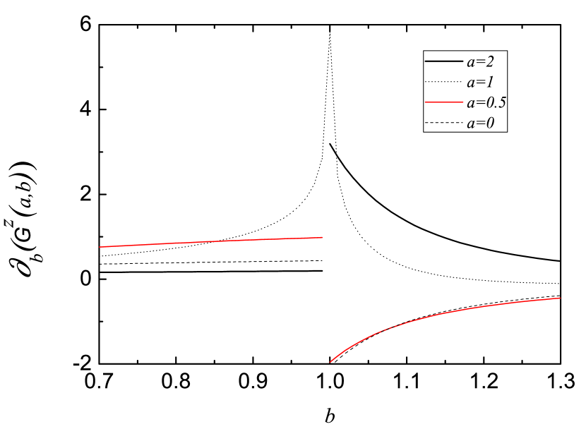
Figure 6: $\gamma=0.6$. $\partial_{b}G^{z}_{1}(a,b)$ with fixed initial magnetic field $a=0,0.5,1,2$.

VI Summary

In summary, starting from a general Hamiltonian which may undergo a QPT with the change of a controllable parameter, we obtain a general conclusion that in a sudden quench system, when the final Hamiltonian is fixed, the behavior of the time-averaged expectation of any observable has close relationship with the gapless excitation of the initial Hamiltonian. This general conclusion, clarified by our example of XY model, to a large extent explains the similarity between the critical phenomena of sudden quench and static system. The long-range correlation is also studied and we find that sudden quench can destroy long-range correlation in the $x$ direction. As we know, the one-spin reduced density matrix can always be written as $\rho=(I+\sum_{\alpha=x,y,z}\langle\sigma_{\alpha}\rangle\sigma_{\alpha})/2$. If considering symmetry breaking effects in XY chain PRA77032325 , we cannot suppose $\langle\sigma_{x}\rangle=0$. Therefore for static case it will be a complex task to solve $\langle\sigma_{x}\rangle$. But for sudden quench, $\langle\sigma_{x}(a,b)\rangle=0$ for $a\neq b$. So our result can help to simplify the calculation of one (two)-site reduced density matrix. This will be useful in studying the entanglement of one site with others for XY model. In addition, the general conclusion can be useful for other quantities and other models.

This work was supported by NSF of China under Grants No. 10821403 and No. 10974234, programs of Chinese Academy of Sciences, 973 grant No. 2010CB922904 and National Program for Basic Research of MOST.

References

- (1) S. Sachdev: Quantum Phase Transition, Cambridge University Press, Cambridge 1999.
- (2) M. Greiner et al., Nature(London) 419, 51 (2002); T. W. B. Kibble, J. Phys. A 9, 1387 (1976); W. H. Zurek, Nature(London) 317, 505 (1985).
- (3) K. Sengupta, S. Powell and S. Sachdev, Phys. Rev. A 69, 053616 (2004).
- (4) W. H. Zurek, U. Dorner and P. Zoller, Phys. Rev. Lett. 95, 105701 (2005).
- (5) J. Dziarmaga, Phys. Rev. Lett. 95, 245701 (2005).
- (6) A. Polkovnikov, Phys. Rev. B 72, 161201(R) (2005).
- (7) A. Sen, U. Sen and M. Lewenstein, Phys. Rev. A 72,052319 (2005).
- (8) B. Damski and W. H. Zurek, Phys. Rev. A 73, 063405 (2006).
- (9) F. M. Cucchietti, B. Damski, J. Dziarmaga and W. H. Zurek, Phys. Rev. A 75, 023603 (2007).
- (10) V. Mukherjee, U. Divakaran, A. Dutta and D. Sen, Phys. Rev. B 76, 174303 (2007).
- (11) K. Sengupta, D. Sen and S. Mondal, Phys. Rev. Lett. 100, 077204 (2008).
- (12) A. Polkovnikov and V. Gritsev, Nat. Phys. 4, 477 (2008).
- (13) M. Rigol, V. Dunjko and M. Olshanii, Nature (London) 452, 854 (2008).
- (14) Y. Li, M. Huo and Z. Song, Phys. Rev. B 80, 054404 (2009).
- (15) M. Rigol et al., Phys. Rev. Lett. 98, 050405 (2007); M. Rigol et al., Phys. Rev. A 74, 053616 (2006).
- (16) D. Patane, A. Silva, F. Sols and L. Amico, Phys. Rev. Lett. 102, 245701 (2009).
- (17) S. Hofferberth, I. Lesanovsky, B. Fischer, T. Schumm, J. Schmiedmayer, Nature 449, 324 (2007).
- (18) G. Roux, Phys. Rev. A 79, 021608(R) (2009).
- (19) E. Barouch, B. M. McCoy and M. Dresden, Phys. Rev. A 2, 1075 (1970); E. Barouch and B. M. McCoy, Phys. Rev. A 3, 786 (1971); E. Barouch and B. M. McCoy, Phys. Rev. A 3, 2137 (1971).
- (20) T. R. de Oliveira, G. Rigolin, M. C. de Oliveira and E. Miranda, Phys. Rev. A 77, 032325 (2008).