Inelastic mechanics of sticky biopolymer networks

Abstract

We propose a physical model for the nonlinear inelastic mechanics of sticky biopolymer networks with potential applications to inelastic cell mechanics. It consists in a minimal extension of the glassy wormlike chain (Gwlc) model, which has recently been highly successful as a quantitative mathematical description of the viscoelastic properties of biopolymer networks and cells. To extend its scope to nonequilibrium situations, where the thermodynamic state variables may evolve dynamically, the Gwlc is furnished with an explicit representation of the kinetics of breaking and reforming sticky bonds. In spite of its simplicity the model exhibits many experimentally established non-trivial features such as power-law rheology, stress stiffening, fluidization, and cyclic softening effects.

1 Introduction

In many studies of cell mechanics and dynamics, the cell is characterized as a viscoelastic body [1, 2, 3]. It is an intriguing question to what extent such mechanical behaviour can be rationalized in terms of comparatively simple polymer physics models. In this respect, the comparison of cell rheological data and minimalistic in vitro reconstituted constructs of the cytoskeleton, such as pure actin solutions [4, 5, 6, 7, 8] or crosslinked actin networks [9, 10, 11, 12, 13, 14], has recently provided many new insights. Important progress has also been achieved in the development of phenomenological mathematical descriptions. This includes approaches related to the tube model [15, 16, 17, 18], tensegrity-based approaches [19, 20, 21], effective-medium models [22, 23, 24], and some others [25, 26]. In particular, the glassy wormlike chain (Gwlc) model [27], a phenomenological extension of the standard Wlc model of semiflexible polymers [28] has been successful in describing a plethora of rheological data for polymer solutions [7, 29] and living cells [30] over many decades in time with a minimum of parameters. However, all these studies were primarily concerned with viscoelastic behaviour, while the latest investigations have underscored the glassy [31, 32, 33] fragile [34, 35], and inelastic [34, 35, 36] character of the mechanical response of living cells. Even for biopolymer networks in vitro, experiments operating in the nonlinear regime had so far to resort to special protocols that minimize plastic flow [37, 8] in order to make contact with dedicated theoretical models.

The aim of the present contribution is to overcome this restriction by extending the Gwlc to situations involving inelastic deformations. As a first step, we concentrate onto reversible inelastic behaviour, where the deformation does not alter the microscopic ground state. The protocol applied by Trepat et al. [34] provides a paradigmatic example. Cells are subjected to a transient stretch such that, after some additional waiting time in the unstretched state, the (linear) material properties of the initial state are recovered. The simplification for the theoretical modelling results from the assumption that not only the macro-state but also the micro-state of the system may to a good approximation be treated as reversible under such conditions; i.e., we assume that the complete conformation of the polymer network, including the transiently broken bonds between adjacent polymers, is constrained to eventually return to its original equilibrium state. For the time-delayed hysteretic response of the network to such protocols one could thus still speak of a viscoelastic (“anelastic”) response in an operational sense, but we refrain from doing so in view of the fundamentally inelastic nature of the underlying stochastic process — in contrast to the reversible softening effects observed in [38], for example. Indeed, by simply allowing bonds to reform in new conformational states, the model developed below can readily be extended to arbitrary irreversible plastic deformations, as will be demonstrated elsewhere [45]. Before entering the discussion of our model, we would also like to point out that the proposed (inelastic) extension of the Gwlc is strongly constrained by identifying the newly introduced parameters with those of the original (viscoelastic) Gwlc model, where possible. Despite its increased complexity, the extended model will therefore enable us to subject the underlying physical picture to a more stringent test than hitherto possible by comparing its predictions to dedicated experiments. Moreover, unlike current state-of-the-art simulation studies [25] it is not limited to rod networks but is firmly routed in a faithful mathematical description of the underlying Brownian polymer dynamics.

This paper is organized as follows. First, we review some basic facts about the Gwlc in section 2.1. Next, in section 2.2, we introduce our extended reversible inelastic version, which we formulate using the notion of an effective interaction potential as in the original construction of the Gwlc in [27]. (A preliminary account of the basic procedure and some of its cell-biological motivation including reversible bond-breaking kinetics has recently been given in a conference proceedings [39].) Sections 3.1 and 3.2 explain the physical mechanism underlying the mechanical response under pulsed and periodically pulsed loading, while section 3.3 illustrates its phenomenology. We demonstrate that the model exhibits the hallmarks of nonlinear cell mechanics: strain/stress stiffening, fluidization, and cyclic softening [34, 35, 36]. Section 3.4 investigates the relevance of the lately quantified structural heterogeneities in networks of semiflexible polymers [40] for the mechanical properties, before we conclude and close with a brief outlook.

2 Theory

2.1 The glassy wormlike chain

The glassy wormlike chain (Gwlc) is a phenomenological extension of the wormlike chain (Wlc) model, the well-established standard model of semiflexible polymers. A broad overview over Wlc and Gwlc dynamics can be found elsewhere [28]. The Wlc describes the mechanics of an isolated semiflexible polymer in an isothermal viscous solvent. In the weakly bending rod approximation, a solution of the stochastic differential equations of motion for the Wlc is possible via a mode decomposition ansatz for the transverse displacement of the polymer contour from the straight ground state. The individual modes labelled by an index $n$ are independent of each other and decay exponentially with rates $\tau_{n}^{-1}$. For convenience, we set the thermal energy $k_{B}T=1$, so that the bending rigidity can be identified with the persistence length $\ell_{p}$, in the following. Using this convention, the Wlc expression for the transverse susceptibility of a polymer of contour length $L$ (with respect to a point force) reads [27]

$$\alpha_{\mbox{\scriptsize{\sc Wlc}}}(\omega)=\frac{L^{3}}{\ell_{p}\pi^{4}}\sum_{n=1}^{\infty}\frac{1}{(n^{4}+n^{2}f/f_{L})(1+i\omega\tau_{n})}.$$ (1)

Here, $f$ is an optional backbone tension, and $f_{L}\equiv\pi^{2}\ell_{p}/L^{2}$ the Euler buckling force for a hinged rod of length $L$. The different powers of $n$ in the denominator give notice of the competition of bending and stretching forces.

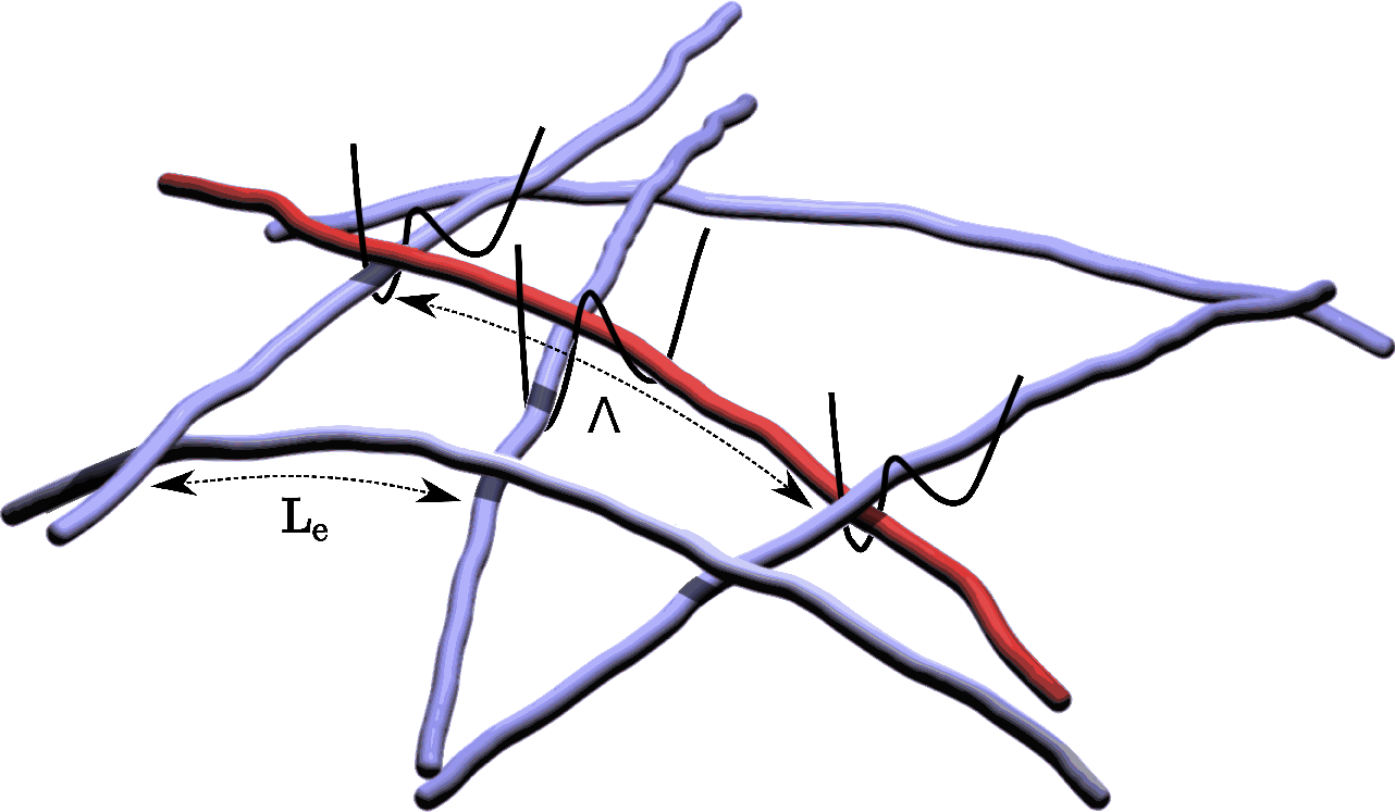
Figure 1: Cartoon of a test polymer (differently coloured) in a network. The trapping of the test polymer is schematically represented by means of an effective interaction (figure 2) indicated by the potential wells at sticky entanglement points, which are on average separated by an contour length $L_{e}$. The test polymer can bind/unbind by overcoming an energy barrier of height $\mathcal{E}$. The average contour length between the closed bonds is $\Lambda$.

In the Gwlc, interactions of the polymer with the surrounding network (e.g. excluded volume interactions or sticky contacts) are reflected in an altered Wlc mode relaxation spectrum [27, 29]. The intuitive — albeit not fully microscopic — picture underlying the formulation of the Gwlc is illustrated in figure 1, which depicts a test polymer reversibly bound to the background network via potential wells at all topological contacts, the so-called entanglement points. Consider now a generic point somewhere along the polymer backbone (not an entanglement point). It can relax freely until the constrictions are being felt, which slow down the contributions from long wavelength bending modes. The Gwlc translates this intuition into a simple prescription for the mode spectrum: the short-wavelength modes are directly taken over from the wormlike chain model, while modes of wavelength $\lambda_{n}$ longer than the typical contour length $\Lambda$ between adjacent bonds are modified to account for the slowdown. Motivated by the physical picture illustrated in figure 1, the slowdown of the relaxation of a wavelength $\lambda_{n}$ is expressed by an Arrhenius factor $\exp\left[\mathcal{E}\left(\lambda_{n}/\Lambda-1\right)\right]$ for breaking $(\lambda_{n}/\Lambda-1)$ potential energy barriers of height $\mathcal{E}$ simultaneously. Accordingly, the phenomenological recipe to turn a Wlc into a Gwlc reads:

$$\tau_{n}\to\tilde{\tau}_{n}=\left\{\begin{array}[]{c c}\tau_{n}&\lambda_{n}<\Lambda\\ \tau_{n}\exp\left[\mathcal{E}(\lambda_{n}/\Lambda-1)\right]&\lambda_{n}\geq\Lambda\end{array}\right..$$ (2)

Upon inserting this into (1) one obtains the Gwlc susceptibility $\alpha_{\mbox{\scriptsize{\sc Gwlc}}}(\omega)$. The microscopic “modulus” for transverse point excitations of a generic backbone element on a test polymer is then defined as the inverse susceptibility, $g_{\mbox{\scriptsize{\sc Gwlc}}}(\omega)=1/\alpha_{\mbox{\scriptsize{\sc Gwlc}}}(\omega)$. An approximate expression for the macroscopic shear modulus is obtained along similar lines [22, 27].

In the original equilibrium Gwlc theory, $\Lambda$ was assumed to be a constant on the order of the entanglement length of the network, $\Lambda\gtrsim L_{e}$. Note, however, that $L_{e}$ is a geometric quantity (which is determined by the polymer concentration and the persistence length) while the contour length $\Lambda$ between closed bonds clearly depends on the state of the bond network. One therefore has to allow for an increase of $\Lambda$ with the number of broken bonds in non-equilibrium applications. This issue is explored in the following.

2.2 Effective interaction potential and bond kinetics

All mechanical quantities calculated within the Gwlc model crucially depend on the interaction length $\Lambda$. In previous applications of the model [7, 27, 30] it was assumed that $\Lambda$ remains constant — equal to its equilibrium value and unaffected by the deformation of the sample. In other words, the equilibrium theory allowed for statistical bond fluctuations but not for a dynamical evolution of the parameters characterizing the thermodynamic state of the bond network. An obvious starting point for generalizations of the model to non-equilibrium situations is therefore to consider the number of closed bonds, and therefore also $\Lambda$, as dynamic variables, dependent on the strain- and stress-history of the network. We now provide a mean-field description to account for such a dynamically evolving bond network. For clarity, we return to the intuitive picture underlying the Gwlc  where the (possibly crosslinker- or molecular-motor-mediated) complex interactions between the polymers are summarized into an effective interaction potential for a test segment against the background, as sketched in figure 2. The same idea has also been used before in many related situations (e.g. [41, 42, 26]).

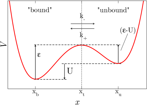
Figure 2: Sketch of the schematic effective interaction potential for a test segment against the background. A polymer segment can either be “bound” by a transient crosslinker or a sticky patch on the backbone of another polymer (left potential well) or “unbound” and merely confined by the surrounding network to a tube like cage (right well). When considering an ensemble of contacts, the fraction of closed bonds depends on the free energy difference $U$ between both states. The transition rates $k_{-}$ and $k_{+}$ between the bound and unbound state depend on the barrier heights $\mathcal{E}$ and $(\mathcal{E}-U)$, respectively. An externally applied force can tilt the potential and favour binding or unbinding events.

The generic potential exhibits three essential features: a well-defined bound state, a well-defined unbound state, and a barrier in between (figure 2). The confining well corresponding to the unbound state represents the tube-like caging of the test polymer within the surrounding network [15, 43, 17]. For ease of notation, we further introduce the dimensionless fraction of closed bonds or, bond fraction

$$\nu(t)\equiv\Lambda_{0}/\Lambda(t)\;,$$ (3)

which is simply the ensemble-averaged fraction of sticky contacts that are actually in the bound state. The minimum bond distance $\Lambda_{0}$ is typically on the order of $L_{e}$, but may be somewhat larger in situations where the bonds are mediated by crosslinker molecules or by partially sterically inaccessible sticky patches (as e.g. for helical molecules [12, 44]).

A quantitatively fully consistent way of calculating the dynamics of $\nu$ would involve solving the full Fokker-Planck equation for a Wlc-Wlc contact — a formidable program to be pursued elsewhere [45]. Here, for the sake of our qualitative purposes, we chose to concentrate onto the physical essence of the discussion, and keep the mathematical structure as simple and transparent as possible. We therefore approximate the dynamics by a simple exponential relaxation as familiar from the standard example of reacting Brownian particles, conventionally described by Kramers theory with a Bell-like force dependence [46, 47]. Using this simplification and assuming a schematic interaction potential as depicted in figure 2, the value of $\nu$ is determined by a competition of bond breaking and bond formation with reaction rates $k_{-}$ and $k_{+}$, respectively. Both rates are represented in the usual adiabatic approximation (meaning that the equilibration inside the wells is much faster than the barrier crossing and external perturbations) by [46]

$$k_{-}\tau_{0}=e^{-\mathcal{E}+(x_{t}-x_{b})f}\;,\qquad k_{+}\tau_{0}=e^{-\mathcal{E}+U-(x_{u}-x_{t})f},$$ (4)

where $\tau_{0}$ is an intrinsic characteristic Brownian time scale for bond breaking and formation, and $f$ is the force pulling on the bond. Noting that the fraction of open bonds is $1-\nu$, we can then write down the following rate equation for the fraction of closed bonds

$$\dot{\nu}(t)\tau_{0}e^{\mathcal{E}}=-(e^{-(x_{u}-x_{t})f(t)+U}+e^{(x_{t}-x_{b})f(t)})\nu(t)+e^{-(x_{u}-x_{t})f(t)+U}.$$ (5)

The time dependence of $\nu(t)$ leads via (3) to an implicit time dependence of the Gwlc-parameter $\Lambda(t)$ and thereby of all observables derived from the Gwlc. The time-dependent force $f(t)$ in (5) may be thought to result from an externally imposed stress protocol or from internal dynamical elements such as molecular motors setting the network under dynamic stress. Hence, via an appropriately chosen set of slowly changing state parameters $f(t)$, $U(t)$, $\mathcal{E}(t)$, … the model can in principle accommodate for the active biological remodelling in living cells and tissues [39]. (For a discussion of the relation between the microscopic $f$ and the macroscopic stress, see [29].) Note that for constant force, the stationary value of $\nu$,

$$\nu_{\rm stat}=\left(1+\exp\left[-U+(x_{u}+x_{b})f_{\rm stat}\right]\right)^{-1},$$ (6)

obtained by setting $\dot{\nu}\equiv 0$, does not depend on $\mathcal{E}$, as it should be (the steady state is independent of the transition state).

3 Results and discussions

3.1 Viscoelastic properties

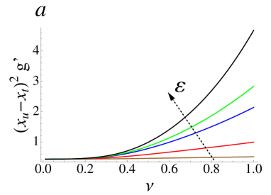
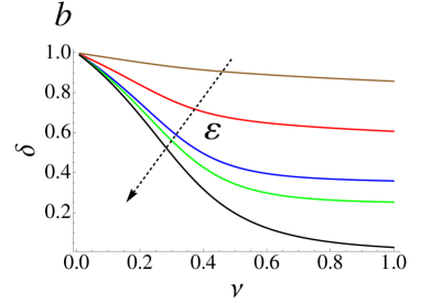
Figure 3: Dependence of the microrheological “modulus” $g_{\mbox{\scriptsize{\sc Gwlc}}}$ on the bond fraction $\nu$ for various values of $\mathcal{E}$ (brown: $\mathcal{E}=0.1$, red: $\mathcal{E}=1$, blue: $\mathcal{E}=5$, green: $\mathcal{E}=10$, black: $\mathcal{E}=\infty$) at a frequency $\omega_{0}\approx 1/10\tau^{-1}_{\Lambda_{0}}$ and a force $f=f_{\Lambda_{0}}/2$ ($\tau_{\Lambda_{0}}$ is the relaxation time of a mode of length $\Lambda_{0}$ and $f_{\Lambda_{0}}$ is the Euler buckling force for a rod of length $\Lambda_{0}$); left: normalized real part $g^{\prime}$; right: loss angle.

Whenever the bond kinetics can be disregarded ($\dot{\nu}=0$), the viscoelastic properties are simply those of the bare Gwlc [27, 7, 29, 30], which can basically be characterized as Wlc short time dynamics followed by a slow, highly stretched logarithmic relaxation resembling power-law rheology with a non-universal exponent within the typical experimental time windows. Strong perturbations (stress or strain) then give rise to a pronounced stiffening due to the steeply nonlinear response of semiflexible polymers under elongation [2]. This well established behaviour can be understood as the canvas against which we aim to discern the characteristic mechanical signatures of the bond kinetics.

An observable that will be of particular interest in the following is the complex microscopic “modulus” $g\equiv g_{\mbox{\scriptsize{\sc Gwlc}}}(\omega_{0},\Lambda_{0}/\nu,f)$, introduced in the previous section. It is used to determine the linear as well as (via a nonlinear update scheme, see A) the nonlinear force response of the system. To understand how the time-dependence (5) of $\nu$ affects this important quantity, it is instructive to first examine the dependence of $g$ on $\nu$. To this end, we formally consider $\nu$ temporarily as an independent variable instead of determining it from (5). Note that this approach nevertheless makes sense as for a fixed set of parameters, $\nu$ can still take any value between zero and one. This is due to the freedom of choosing an initial state, which can be imagined to have evolved from the prior deformation history.

For fixed other parameters, both the real part $g^{\prime}$ (figure 3a) and the imaginary part $g^{\prime\prime}$ of $g$ increase monotonically with $\nu$. We emphasize that $g^{\prime\prime}$ is not simply proportional to $g^{\prime}$ and therefore the loss angle $\delta=\arctan(g^{\prime\prime}/g^{\prime})$ also depends on $\nu$ (figure 3b). For small $\nu$, the loss angle is large, corresponding to fluid-like behaviour. With increasing $\nu$, the system becomes more solid-like. Increasing the barrier height $\mathcal{E}$ makes the dependence of $g$ on $\nu$ more pronounced (figure 3). Conversely, as can be expected, the dependence on the barrier height $\mathcal{E}$ vanishes with decreasing bond fraction $\nu$. Note that due to the boundary conditions the limit of a Newtonian fluid ($\delta=\pi/2$) is not recovered when formally taking the limit of vanishing bond fraction ($\nu\to 0$, $\Lambda\to\infty$). Finally, the potential difference $U$ solely determines the dynamics of $\nu$ via (5), and therefore influences the modulus $g$ solely through the equilibrium value for $\nu$.

After these general considerations, we now concentrate on the nonlinear and non-equilibrium dynamic response of the extended inelastic Gwlc model, which results from the coupled relaxation of the viscoelastic polymer network and the transient bond network.

3.2 Stress-stiffening versus rate-dependent yielding

A convenient way to characterize the mechanical properties of an inelastic material is a force-displacement curve. For a perfectly linear elastic (Hookean) body, it would simply consist of a straight line, whereas a perfectly plastic body would feature as a rectangle delineated by a yield force $f_{\rm y}$ and an arbitrary plastic strain value. For our qualitative purpose, we identify the average transverse displacement of the test polymer segment (which is used to determine the force response, see A) with the reaction coordinate $x$ of the schematic potential sketched in figure 2; and we identify the force $f$ entering the reaction rates with the backbone tension of the test polymer. As a characteristic length scale for the transverse displacements we use the width $(x_{u}-x_{t})$ of the effective confinement potential, which is a measure of a typical mean-square displacement of the polymer in the unbound state. Using this convention, we now consider the effect of a time-symmetric displacement pulse on the evolution of the force $f(t)$ and bond fraction $\nu(t)$. For technical convenience, we use a Gaussian shape for the displacement pulses, but the qualitative conclusions to be drawn are largely independent of the precise protocol. The duration of the displacement pulse, which sets the time scale for the dynamic response, is used as the unit of time in the following. Here, we are not interested in short-time tension-propagation and single-polymer dynamics [48], hence a lower bound for pertinent pulse durations is provided by the interaction time scale $\tau_{\Lambda_{0}}\simeq\tau_{0}$. On the other hand, for pulse durations longer than $\tau_{0}e^{\mathcal{E}}$ the system deformation would be quasistatic so that no genuinely dynamic effects of the bond kinetics could be observed.

For a small Gaussian displacement pulse of relative amplitude $0.73$ (c.f. figure 4a and A), the shape of the curve predicted by our inelastic Gwlc model shows all features of a viscoelastic medium (figure 4b, blue dashed curve). It starts with a nearly linear regime for relative displacements $\lesssim 0.4$, where a weak stiffening sets in. Due to dissipation in the medium, the path back to the initial state takes its course at lower force, which causes a weak hysteresis. This is essentially the viscoelastic response that already the bare Gwlc model would have predicted.

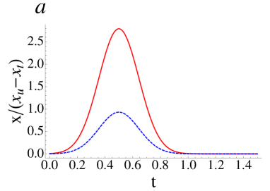
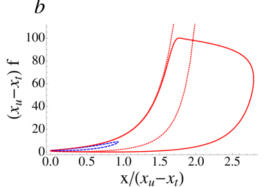
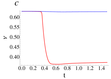
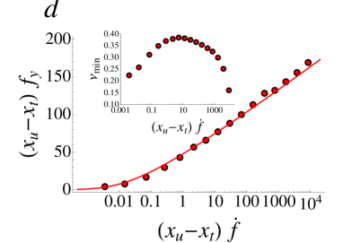
Figure 4: Transition from a stiffening to a softening response at a rate-dependent, operationally defined yield force $f_{\rm y}$: Gaussian deformation pulses ($a$) with relative displacement amplitudes of $0.73$ (dashed) and $2.2$ (solid); corresponding force-displacement curves and bond fraction evolutions ($b$, $c$; dotted curve in $b$: response of a Gwlc without bond breaking); order-of-magnitude estimate for the rate-dependence of the yield force, (7) with const.$=2.2$, versus the numerically obtained maximum forces of the force-displacement curves for various mean force rates ($d$); the minimum bond fraction ($d$, inset) depends non-monotonically on the force rate; $\mathcal{E}=10.5$, $U=2$, $\tau_{0}=0.004$, $(x_{t}-x_{b})/(x_{u}-x_{t})=0.07$, $\Lambda_{0}=22.3$.

For a larger relative deformation amplitude of $2.2$, however, the predictions of the bare Gwlc and the inelastic Gwlc diverge. The bare Gwlc predicts a strong stiffening (figure 4b, red dotted curve), whereas the full model exhibits an initial stiffening regime followed by a pronounced softening (figure 4b, solid red curve). A very interesting observation is that “softening” in this case does not only mean a decrease of the slope of the force-extension curve, but that the slope actually becomes negative over an extended parameter region, once an operationally defined threshold force $f_{\rm y}$ is exceeded. This “flow state” bears more resemblance to plastic flow than to viscoelastic relaxation. The reason for this qualitatively new phenomenon is the force-induced bond breaking. Theoretically this is best exemplified by the time-dependence of the (experimentally not easily accessible) fraction $\nu(t)$ of closed bonds (figure 4c). A glance at the bond fraction during the weak deformation scenario (figure 4c, blue dashed curve) reveals how the limit of a bare Gwlc is recovered, namely whenever the deformation is not sufficiently violent and persistent to significantly decrease the fraction of closed bonds. For the large deformation scenario, in contrast, the bond fraction stays only initially constant (figure 4c, solid red curve). As a consequence of the large strain the force rises steeply, as can be seen from the strong stiffening in figure 4b (solid red curve). At the yield force, the bond fraction suddenly decreases to nearly half of its initial value during a very short time. The decrease in the bond fraction is accompanied by a somewhat slower drop in the force, which is reflected in the sudden softening of the force-displacement curve. The bond fraction eventually recovers on a much slower time scale, which is roughly given by $\tau_{0}\exp(\mathcal{E}-U)$. Note that even though the effects of the inelastic response dominate the stress-strain curve, the viscoelastic relaxations from the underlying Gwlc model are still present. They could hardly be disentangled from the inelastic contributions, though, without an underlying faithful model of the viscoelastic response at hand.

In summary, we observe a competition between force-amplitude dependent stress-stiffening and force-rate dependent yielding events. If the backbone force stays much smaller than the yield force, the adaptation of the bond network requires an adiabatically long time, on the order of the bond lifetime $\tau_{0}e^{\mathcal{E}}$, so that plain viscoelastic Gwlc behaviour is observed on the pulse time scale. In contrast, if the backbone tension $f$ reaches the yield force $f_{\rm y}$, the bond fraction declines sharply, thereby switching the response from the Wlc/Gwlc-typical stiffening to a pronounced softening.

The rate dependence of the yield force $f_{\rm y}$ can be estimated by setting the time it takes to reach the yield force, $f_{\rm y}/\dot{f}$, equal to the force-dependent time scale of bond opening, $k^{-1}_{-}(f)$, from (4),

$$f_{\rm y}\dot{f}^{-1}\simeq k_{-}^{-1}(f_{\rm y})\quad\Rightarrow\quad(x_{t}-x_{b})f_{\rm y}\approx{\rm LW}\left(\mbox{const.}\times(x_{t}-x_{b})\tau_{0}e^{\mathcal{E}}\dot{f}\right).$$ (7)

Here, LW$(x)$ is the positive real branch of the Lambert W function. In figure 4d, this estimate is compared with results from numerical evaluations for Gaussian displacement pulses at different average rates. Apart from the numerical errors, the slight deviations from the estimate may be attributed to the fact that the force rate is not constant for the Gaussian protocol. They can be mostly eliminated by using force ramp protocols of various slopes instead of the Gaussian displacement pulses. For not too low rates, the rate dependence can be approximated by the even simpler relation

$$(x_{t}-x_{b})f_{\rm y}\approx(\mathcal{E}+\ln\dot{f}\tau_{0}+\mbox{const.})\;,$$ (8)

where the force rate has to be normalized by a suitable force scale.

The minimum bond fraction reached during the application of the pulse, which we interpret as a measure of the degree of fluidization, depends non-monotonically on the rate (figure 4d, inset). Qualitatively, this can be understood by noticing that two different factors influence the fluidization, namely the maximum force attained during deformation and the time over which the force is applied. The maximum force is simply the yield force $f_{\rm y}$, with the rate dependence in (7) and figure 4d, while the reciprocal rate itself sets the time scale. For high rates $(x_{u}-x_{t})\dot{f}\gtrsim 1$ (in our example) the rate-dependence of the maximum force wins and the minimum $\nu$ reached decreases with increasing rate. For low rates, where the rate-dependence of the maximum force is much weaker (figure 4d) the minimum $\nu$ decreases with increasing pulse duration, viz. decreasing rate. Note that for slow pulses (low rates), the bond fraction after the pulse may be quite different from the minimum $\nu$, as significant recovery may already take place during the pulse.

3.3 Transient remodelling and cyclic softening

The substantial changes in the material properties accompanying bond breaking can be exemplified by monitoring the linear elastic modulus $g^{\prime}(\omega_{0})$ (measured at a fixed frequency $\omega_{0}$) in response to a strain pulse (figure 5a). Apart from the usual Wlc/Gwlc-typical stress-stiffening below the threshold force $f_{\rm y}$, the modulus is seen to drop below the value it had before the deformation pulse, where it apparently saturates (remember that the deformation vanishes for $t>1$ and that the recovery takes roughly a time $\tau_{0}e^{\mathcal{E}-U}\gg 1$). We thus observe what we call a “passive”, “physical” remodelling of the bond network as opposed to the “active”, “biological” remodelling of the cytoskeleton of living cells in response to external stimuli. These passive remodelling effects have recently been observed for human airway smooth muscle cells [34]. (A more quantitative discussion of the relation to the experimental observations will be given elsewhere.) The fact that the deformation pulse leads to a decrease in $g^{\prime}$ and an increase in the loss angle $\delta$ (figure 5c) suggests the notion of fluidization [34].

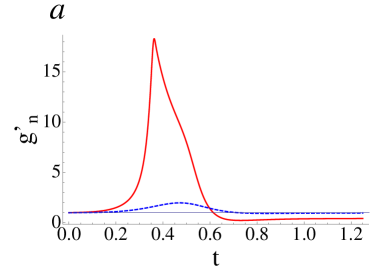
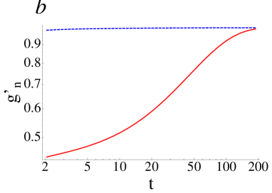
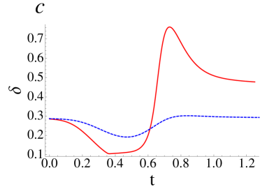
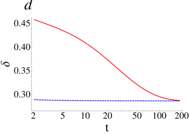
Figure 5: The internal force $f$ and the bond fraction $\nu$ largely determine the storage modulus $g^{\prime}$ and the loss angle $\delta$: normalized storage modulus $g^{\prime}_{\rm n}$ ($a$) and loss angle $\delta$ ($c$) during displacement pulses of large and small amplitudes, 2.2 (solid), 0.73 (dashed); the stronger deformation pulse causes a strong and persistent overshoot of the loss angle, indicating fluidization; slow recovery after the pulse, ($b$, $d$); parameters as in figure 4, $\omega_{0}=3$.

The passive remodelling described here is a transient phenomenon, because, after cessation of the external perturbations, the bond fraction will eventually recover its equilibrium value. This indicates that also the change in the system properties is a transient effect, which is demonstrated by the recovery from fluidization in figure 5 b & d. Thus, while the fluidization resembles a plastic process on short time scales, on long times scales, the phenomenology is more similar to pseudo- and superelasticity as observed in shape-memory alloys [49].

To demonstrate that the transient passive remodelling also affects the nonlinear material properties, we consider a series of three pulses, next (figure 6). The force response to such a protocol is depicted in figure 6b. The force-displacement curve for the second stretching (second left branch of the solid curve) is less steep than for the first stretching (very left branch of the solid curve) and the yield force is lower. This indicates a cyclic softening, or viscoelastic shake-down effect, closely related to the fluidization of the network by strain. The strength of the shake-down depends on the fraction of transiently broken bonds, and hence on the rate as well as on the amplitude of the applied deformation (c.f. figure 6c, solid red curve). Upon repeated application of deformation pulses the force-displacement curves settle on a limit-curve that is essentially preconditioned by the initial deformation pulse and the inelastic work it performed on the sample. For more gentle protocols that only break a smaller fraction of bonds, the initial fluidization would be not as pronounced and one would obtain a gradual shake-down, which converges to a limit curve only after many cycles.

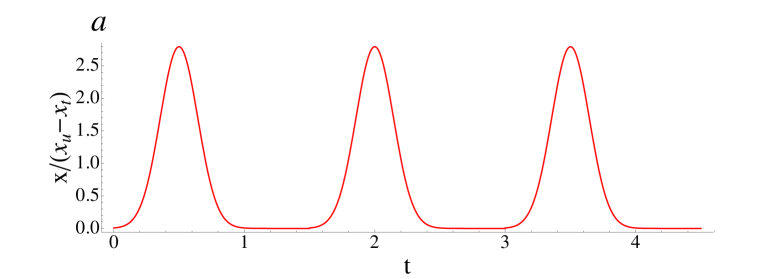
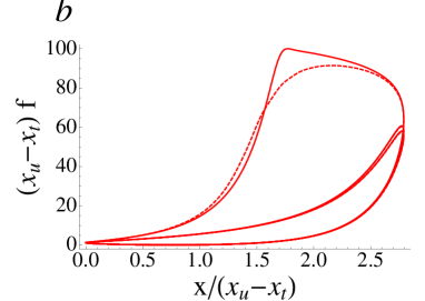
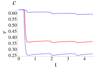
Figure 6: Protocol ($a$) and response ($b$, $c$) for three subsequent Gaussian strain pulses; force-displacement curves ($b$) for a single minimum interaction distance ($\Lambda_{0}=22.3$, solid) and for a distribution of $\Lambda_{0}$ according to [40] with mean $\overline{\Lambda_{0}}=22.3$ (dashed); the bond fraction $\nu$ ($c$) for $\Lambda_{0}=0.5\,\overline{\Lambda_{0}}$ (dash-dotted), $\overline{\Lambda_{0}}$ (solid), and $2\overline{\Lambda_{0}}$ (dashed); other parameters as in figure 4.

3.4 Introducing multiple length scales

So far, we have assumed that there is one well-defined characteristic length scale $\Lambda_{0}$ for the polymer interactions, which is on the order of the entanglement length $L_{e}$ and interpreted as the minimum average contour distance between adjacent bonds of the test polymer with the background network. This is clearly a mean-field assumption. Recent combined experimental and theoretical studies have established that the local tube diameter and entanglement length in pure semiflexible polymer solutions actually exhibit a skewed leptocurtic distribution with broad tails [40]. To include this information in the above analysis is not straightforward, since the elastic interactions between regions of different entanglement length are not known, a priori. For the sake of a first qualitative estimate, the simplest procedure seems to be to average the above results over a distribution of $\Lambda_{0}$, corresponding to a parallel connection of independent entanglement elements. Qualitatively, this renders the abrupt transition from stiffening to softening somewhat smoother (c.f. figure 6b, dashed curve). Moreover, the initial stiffening is slightly more pronounced. This is due to the contributions of $\Lambda_{0}<\overline{\Lambda}_{0}$, which exhibit both stronger stiffening and fluidization. Nevertheless, all qualitative features — like stiffening and remodelling effects and a “flow state” indicating fluidization or inelastic shakedown — can still be well discerned. This is consistent with the assumption that pure semiflexible polymer solutions are at least qualitatively well described by a single entanglement length [22, 50, 27, 17, 18].

4 Conclusions and outlook

We have presented a theoretical framework for a polymer-based description of the inelastic nonlinear mechanical behaviour of sticky biopolymer networks. We represented the polymer network on a mean-field level by a test polymer described by the phenomenologically highly successful Gwlc model. Beyond the equilibrium statistical fluctuations captured by the original model, we additionally allowed for a dynamically evolving thermodynamic state variable $\Lambda(t)$ characterizing the network of thermo-reversible sticky bonds, which is updated dynamically upon bond breaking according to an appropriate rate equation. Within our approximate treatment we could obtain a number of robust and qualitatively interesting results, which are not sensitive to the precise parameter values chosen, nor to the choice of the transverse rather than the longitudinal susceptibility in (1). For sufficiently strong deformations, changes in the mean fraction of closed bonds, reflected in $\Lambda(t)$, can influence material properties to a degree at which the material behaves qualitatively different from the usual viscoelastic paradigm. In particular, our theory predicts a pronounced fluidization response, which develops upon strong deformations on top of the intrinsic viscoelastic stiffening response provided by the individual polymers. After cessation of loading, the system slowly recovers its initial state. These observations are in qualitative agreement with recently published experimental results obtained for living cells [34], and a more quantitative comparison with dedicated measurement results for cells and in vitro biopolymer networks will be the subject of future work. We found the yield force for the onset of the fluidization to be sensitive to the deformation rate. Moreover, the fluidization response was shown to be accompanied by a cyclic softening or shake-down effect. Taking into account the spatial heterogeneity of biopolymer solutions by a distribution of entanglement lengths leads to a smoothing of the force-displacement curves without affecting their qualitative characteristics. One may still expect qualitatively new effects in situations with unusually broad distributions of entanglement lengths, such as for strongly heterogeneous (e.g. phase separating) networks.

A parameter that was found to be very important for cells [51] but has not been discussed much in this contribution is the prestressing force $f_{0}$ (see appendix A), which is present in adhering cells even in the absence of external driving. Experimentally, it was established that increasing prestress is correlated with a higher stiffness of adhering cells [51] which in turn is correlated with a higher stiffness of the substrate [52]. When naively treating the prestressing force just as an additive contribution to the overall force, our model predicts the opposite: the additional force breaks more bonds and the network becomes softer and more fluid-like. To reconcile these apparently contradicting trends, one can appeal to the notion of homeostasis, which essentially amounts to postulating that the cell actively adapts its structure such that a certain set of thermodynamic state variables remain in a physiologically sensible range [39]. This basically implies that the cell will respond to stiff substrates or persistent external stresses by a biological remodelling that corresponds to an increase of $\mathcal{E}$ and $U$, and possibly to a decrease of $\Lambda_{0}$. By adapting also the internal prestress $f_{0}$, the cell may then avoid, apart from the structural collapse, an equally undesirable loss of flexibility. We note, however, that internal stresses are indeed observed to disrupt the cytoskeleton, as implied by the simple physical theory presented here, if they are not permanently balanced by a substrate [53].

Even though the nonlinear effects presented in this contribution depend crucially on the bond kinetics, it should not be overlooked that the Gwlc is an equally indispensable ingredient of the complete theory. First, it provides the constitutive relation that gives the force in response to an infinitesimal displacement, which in turn governs the bond kinetics. Secondly, the time-dependent linear susceptibility strongly filters the dynamic remodelling of the bond network in practical applications, in which one rarely has access to the microstate of the underlying bond network. In summary, the extended model thus integrates experimentally confirmed features of the Gwlc response such as slow relaxation, power-law rheology, viscoelastic hysteresis, and shear stiffening with a simple bond kinetics scheme, which allows less intuitive complex nonlinear physical remodelling effects like fluidization and inelastic shake-down to be addressed.

Finally, we want to point out that it is straightforward to extend the above analysis in a natural way to account for irreversible plastic deformations [45]. To this end, one has to allow for the possibility that the transiently broken bonds reform somewhere else than at their original sites (as always assumed in the foregoing discussion) after strong deformations with finite residual displacement. This can be included by accommodating an additional term acting as a “slip rate” in (5) [45].

Appendix A Obtaining force-displacement curves and solving for $\nu$

The deformation pulse protocol used in this paper is

$$\Gamma(t)=\gamma_{0}\exp\left(-\frac{(t-\tau)^{2}}{\sigma^{2}}\right).$$ (9)

To obtain the full nonlinear response of the (extended) Gwlc to the displacement protocol (9), we make use of the superposition principle: We know that the Fourier transform of $g_{\mbox{\scriptsize{\sc Gwlc}}}(\omega,\Lambda,f)/(i\omega)$ is the linear response to a small displacement step. After decomposing a finite displacement into infinitesimal displacement steps and a partial integration, we write

$$f_{\mbox{\scriptsize{\sc Gwlc}}}(t)=\int_{-\infty}^{\infty}\!\!\!dt^{\prime}\int_{-\infty}^{\infty}\frac{d\omega}{\sqrt{2\pi}}\;g_{\mbox{\scriptsize{\sc Gwlc}}}\left(\omega,\Lambda(t),f_{\mbox{\scriptsize{\sc Gwlc}}}(t)\right)e^{-i\omega(t-t^{\prime})}\Gamma(t^{\prime}).$$ (10)

Note that the right hand side of (10) depends on $f_{\mbox{\scriptsize{\sc Gwlc}}}(t)$, rendering it a highly nonlinear implicit equation. Using (9) and integrating by parts, we obtain

$$f_{\mbox{\scriptsize{\sc Gwlc}}}(t)=\sqrt{2}\gamma_{0}\sigma\int_{0}^{\infty}\!\!\!\!d\omega\,e^{-i\omega(t-\tau)}g_{\mbox{\scriptsize{\sc Gwlc}}}(\omega,\Lambda(t),f_{\mbox{\scriptsize{\sc Gwlc}}}(t))e^{-\frac{\sigma^{2}\omega^{2}}{4}}.$$ (11)

The next step is to identify a connection between the force in (5) and $f_{\mbox{\scriptsize{\sc Gwlc}}}$(t). A finite prestressing force $f_{0}$ is introduced mainly for technical reasons, namely to avoid the unphysical region of negative (i.e. compressive) backbone stress, which would buckle the polymers. While the physics of the prestressed network can essentially be mapped back to that of a network without prestress by a renormalization of the parameters $\mathcal{E}$ and $U$, prestress may also be seen as an important feature: indeed, the cytoskeleton of adhered cells is well known to be under permanent prestress, and suspended cells seem prone to spontaneous shape oscillations that could be indicative of a propensity of the cells to set themselves under prestress [39]. In the context and on the longer time scales of the biological remodelling of the cytoskeleton it would therefore make sense to think of $f_{0}$ as a dynamic force generated by molecular motors and polymerization forces. For the following, however, we take the prestress to be constant so that the force entering (5) is

$$f(t)=f_{0}+f_{\mbox{\scriptsize{\sc Gwlc}}}(t).$$ (12)

We now face the problem that (10) is an implicit equation for $f_{\mbox{\scriptsize{\sc Gwlc}}}(t)$, which depends on $\nu(t)$, which in turn depends via $f(t)$ on $f_{\mbox{\scriptsize{\sc Gwlc}}}(t)$. We therefore use a two-step Euler scheme: As initial values for $f$ and $\nu$, we choose the prestressing force, $f(t=0)=f_{0}$, and the steady-state value under the prestressing force, $\nu(t=0)=\nu(t\to\infty|f=f_{0})$, respectively. We then choose a sufficiently small time step $\Delta t$ and apply the following iterative rule:

$$f(k\Delta t) \approx f_{0}+f_{GWLC}\left(k\Delta t|f((k-1)\Delta t,\nu((k-1)\Delta t)\right)$$ (13)

$$\dot{\nu}(k\Delta t) \approx \dot{\nu}(k\Delta t|f(k\Delta t)),$$ (14)

where $k\in\mathbb{N}_{+}$. In the limit $\Delta t\to 0$, this procedure converges to the exact solution.

References

- [1] Y Fung 1993 Biomechanics: Mechanical Properties of Living Tissues Springer.
- [2] FC MacKintosh, J Käs and P Janmey 1995 Elasticity of semiflexible biopolymer networks Phys. Rev. Lett. 75 4425.
- [3] K Kruse, JF Joanny, F Jülicher, J Prost and K Sekimoto 2004 Asters, vortices and rotating spirals in active gels of polar filaments Phys. Rev. Lett. 92 78101.
- [4] T Gisler and DA Weitz 1999 Scaling of the microrheology of semidilute F-actin solutions Phys. Rev. Lett. 82 1606–1609.
- [5] TG Mason, T Gisler, K Kroy, E Frey and DA Weitz 2000 Rheology of F-actin solutions determined from thermally driven tracer motion J Rheol. 44 917.
- [6] ML Gardel, MT Valentine, JC Crocker, AR Bausch and DA Weitz 2003 Microrheology of entangled F-actin solutions Phys. Rev. Lett. 91 158302.
- [7] C Semmrich, T Storz, J Glaser, R Merkel, AR Bausch and K Kroy 2007 Glass transition and rheological redundancy in F-actin solutions Proc. Nat. Acad. Sci. USA 104 20199–20203.
- [8] C Semmrich, RJ Larsen and AR Bausch 2008 Nonlinear mechanics of entangled F-actin solutions Soft Matter 4 1675–1680.
- [9] ML Gardel, F Nakamura, J Hartwig, JC Crocker, TP Stossel and DA Weitz 2006 Stress-dependent elasticity of composite actin networks as a model for cell behavior Phys. Rev. Lett. 96 88102.
- [10] R Tharmann, M Claessens and AR Bausch 2007 Viscoelasticity of isotropically cross-linked actin networks Phys. Rev. Lett. 98 88103.
- [11] Y Luan, O Lieleg, B Wagner and AR Bausch 2008 Micro- and macrorheological properties of isotropically cross-linked actin networks Biophys. J 94 688–693.
- [12] M Claessens, C Semmrich, L Ramos and AR Bausch 2008 Helical twist controls the thickness of F-actin bundles Proc. Nat. Acad. Sci. USA 105 8819.
- [13] KE Kasza, F Nakamura, S Hu, P Kollmannsberger, N Bonakdar, B Fabry, TP Stossel, N Wang and DA Weitz 2009 Filamin a is essential for active cell stiffening but not passive stiffening under external force Biophys. J 96 4326–4335.
- [14] GH Koenderink, Z Dogic, F Nakamura, PM Bendix, FC MacKintosh, JH Hartwig, TP Stossel and DA Weitz 2009 An active biopolymer network controlled by molecular motors Proc. Nat. Acad. Sci. USA 106 15192.
- [15] J Käs, H Strey and E Sackmann 1994 Direct imaging of reptation for semiflexible actin filaments Nature(London) 368 226–229.
- [16] DC Morse 1999 Viscoelasticity of concentrated isotropic solutions of semiflexible polymers. 3. Nonlinear rheology Macromolecules 32 5934–5943.
- [17] DC Morse 2001 Tube diameter in tightly entangled solutions of semiflexible polymers Phys. Rev. E 63 31502.
- [18] H Hinsch, J Wilhelm and E Frey 2007 Quantitative tube model for semiflexible polymer solutions Eur. Phys. J E 24 35–46.
- [19] P Canadas, VM Laurent, C Oddou, D Isabey and S Wendling 2002 A cellular tensegrity model to analyse the structural viscoelasticity of the cytoskeleton J Theor. Biol. 218 155–173.
- [20] C Sultan, D Stamenović and DE Ingber 2004 A computational tensegrity model predicts dynamic rheological behaviors in living cells Ann. Biomed. Eng. 32 520–530.
- [21] P Cañadas, S Wendling-Mansuy and D Isabey 2006 Frequency response of a viscoelastic tensegrity model: Structural rearrangement contribution to cell dynamics J Biomech. Eng. 128 487.
- [22] F Gittes and FC MacKintosh 1998 Dynamic shear modulus of a semiflexible polymer network Phys. Rev. E 58 1241–1244.
- [23] C Storm, JJ Pastore, FC MacKintosh, TC Lubensky and PA Janmey 2005 Nonlinear elasticity in biological gels. Nature 435 191.
- [24] CP Broedersz, C Storm and FC MacKintosh 2008 Nonlinear elasticity of composite networks of stiff biopolymers with flexible linkers Phys. Rev. Lett. 101 118103.
- [25] JA Åström, PBS Kumar, I Vattulainen and M Karttunen 2008 Strain hardening, avalanches and strain softening in dense cross-linked actin networks Phys. Rev. E 77 51913.
- [26] P Kollmannsberger and B Fabry 2009 Active soft glassy rheology of adherent cells Soft Matter 5 1771–1774.
- [27] K Kroy and J Glaser 2007 The glassy wormlike chain New J Phys. 9 416.
- [28] K Kroy 2008 Dynamics of wormlike and glassy wormlike chains Soft Matter 4 2323–2330.
- [29] J Glaser, O Hallatschek and K Kroy 2008 Dynamic structure factor of a stiff polymer in a glassy solution Eur. Phys. J E 26 123–136.
- [30] K Kroy and J Glaser 2009 Rheological redundancy — from polymers to living cells AIP Conf. Proc. 1151 52–55.
- [31] B Fabry and JJ Fredberg 2003 Remodeling of the airway smooth muscle cell: are we built of glass? Respir. Physiol. Neurobiol. 137 109–124.
- [32] L Deng, X Trepat, JP Butler, E Millet, KG Morgan, DA Weitz and JJ Fredberg 2006 Fast and slow dynamics of the cytoskeleton Nat. Mater. 5 636–640.
- [33] EH Zhou, X Trepat, CY Park, G Lenormand, MN Oliver, SM Mijailovich, C Hardin, DA Weitz, JP Butler and JJ Fredberg 2009 Universal behavior of the osmotically compressed cell and its analogy to the colloidal glass transition Proc. Nat. Acad. Sci. USA 106 10632.
- [34] X Trepat, L Deng, SS An, D Navajas, DJ Tschumperlin, WT Gerthoffer, JP Butler and JJ Fredberg 2007 Universal physical responses to stretch in the living cell Nature 447 592+.
- [35] R Krishnan, CY Park, YC Lin, J Mead, RT Jaspers, X Trepat, G Lenormand, D Tambe, AV Smolensky, AH Knoll, et al. 2009 Reinforcement versus fluidization in cytoskeletal mechanoresponsiveness PLoS ONE 4 .
- [36] P Fernandez and A Ott 2008 Single cell mechanics: Stress stiffening and kinematic hardening Phys. Rev. Lett. 100 238102.
- [37] J Xu, Y Tseng and D Wirtz 2000 Strain hardening of actin filament networks. regulation by the dynamic cross-linking protein alpha-actinin J Biol. Chem. 275 35886.
- [38] O Chaudhuri, SH Parekh and DA Fletcher 2007 Reversible stress softening of actin networks Nature 445 295.
- [39] L Wolff and K Kroy 2009 Mechanical stability: a construction principle for cells Diffusion Fundamentals 11 56.
- [40] J Glaser, D Chakraborty, K Kroy, I Lauter, M Degawa, N Kirchgessner, B Hoffmann, R Merkel and M Giesen 2009 Tube width fluctuations in f-actin solutions arXiv:0910.5864.
- [41] GI Bell 1978 Models for specific adhesion of cells to cells Science 200 618–627.
- [42] U Schwarz, T Erdmann and I Bischofs 2006 Focal adhesions as mechanosensors: The two-spring model BioSystems 83 225–232.
- [43] MA Dichtl and E Sackmann 2002 Microrheometry of semiflexible actin networks through enforced single-filament reptation: Frictional coupling and heterogeneities in entangled networks Proc. Nat. Acad. Sci. USA 99 6533.
- [44] G Grason and R Bruinsma 2008 Chirality and equilibrium biopolymer bundles Phys. Rev. Lett. 99 98101.
- [45] L Wolff, J Bullerjahn and K Kroy unpublished.
- [46] E Evans and K Ritchie 1997 Dynamic strength of molecular adhesion bonds Biophys. J 72 1541–1555.
- [47] W Feneberg, M Westphal and E Sackmann 2001 Dictyostelium cells’ cytoplasm as an active viscoplastic body Eur. Biophys. J 30 284–294.
- [48] O Hallatschek, E Frey and K Kroy 2007 Tension dynamics in semiflexible polymers. I. Coarse-grained equations of motion Phys. Rev. E 75 .
- [49] L Delaey, RV Krishnan, H Tas and H Warlimont 1974 Thermoelasticity, pseudoelasticity and the memory effects associated with martensitic transformations J Mater. Sci. 9 1521–1535.
- [50] AR Bausch and K Kroy 2006 A bottom-up approach to cell mechanics Nat. Phys. 2 231–238.
- [51] N Wang, IM Tolic-Norrelykke, JX Chen, SM Mijailovich, JP Butler, JJ Fredberg and D Stamenovic 2002 Cell prestress. I. Stiffness and prestress are closely associated in adherent contractile cells Am. J. Physiol. Cell Physiol 282 C606–C616.
- [52] D Discher, P Janmey and Y Wang 2005 Tissue cells feel and respond to the stiffness of their substrate Science 310 1139–1143.
- [53] G Salbreux, JF Joanny, J Prost and P Pullarkat 2007 Shape oscillations of non-adhering fibroblast cells Phys. Biol. 4 268–284