QCDMAPT: program package for
Analytic approach to QCD

A.V. Nesterenko^a, and C. Simolo^b

^aBLTPh, Joint Institute for Nuclear Research, Dubna, 141980, Russian Federation

^bISAC–CNR, I–40129, Bologna, Italy

 

Abstract

A program package, which facilitates computations in the framework of Analytic approach to QCD, is developed and described in details. The package includes the explicit expressions for relevant spectral functions calculated up to the four–loop level and the subroutines for necessary integrals.

PACS: 11.15.Tk; 11.55.Fv; 12.38.Lg

Key words: Nonperturbative QCD; Dispersion relations

 

PROGRAM SUMMARY

Manuscript Title: QCDMAPT: program package for Analytic approach to QCD
Authors: A.V. Nesterenko and C. Simolo
Program Title: QCDMAPT
Journal Reference:
Catalogue identifier:
Licensing provisions: none
Programming language: Maple 9 and higher
Computer: Any which supports Maple 9
Operating system: Any which supports Maple 9
Keywords: Nonperturbative QCD; Dispersion relations
PACS: 11.15.Tk, 11.55.Fv, 12.38.Lg
Classification: 11.1, 11.5, 11.6
Nature of problem: Subroutines helping computations within Analytic approach to QCD
Solution method: A program package for Maple is provided. It includes the explicit expressions for relevant spectral functions and the subroutines for basic integrals used in the framework of Analytic approach to QCD.
Running time: Template program running time is about a minute (depends on CPU)

1 Introduction

The strong interactions display two fundamental features, namely, the asymptotic freedom (at high energies) and color confinement (at low energies). The first feature allows one to study the strong interaction processes in the ultraviolet domain by making use of perturbation theory. However, theoretical description of hadron dynamics at low energies requires nonperturbative methods.

In general, there is a variety of nonperturbative approaches to handle the strong interaction processes at low energies. In this work we will focus on the so–called “dispersive” (or “analytic”) approach to Quantum Chromodynamics (QCD). The basic idea of this approach is to merge the perturbative results with the nonperturbative constraints arising from relevant dispersion relations. In turn, this eliminates some intrinsic difficulties of perturbation theory and extends its range of applicability towards the infrared domain. One of the possible implementations of this approach within QCD is the so–called “massless” Analytic Perturbation Theory [1, 2, 3]. The latter has been successfully employed in the studies of various strong interaction processes (see, e.g., papers [4, 5, 6, 7, 8, 9, 10, 11, 12, 13, 14], reviews [3, 15, 16] and references therein). The incorporation of effects due to the nonvanishing mass of lightest hadron state has been implemented into approach in hand within the so–called “massive” Analytic Perturbation Theory, see Refs. [17, 18] for the details.

A central object of the current approach is the so–called spectral function, which can be calculated by making use of the strong running coupling $\alpha_{\mbox{\scriptsize s}}(Q^{2})$ (see Sect. 3). At the one–loop level the perturbative running coupling and relevant spectral function have a quite simple form (Eqs. (32) and (9), respectively). However, at the higher loop levels the strong running coupling has a rather cumbersome structure, and the calculation of corresponding spectral functions represents a rather complicated task.

The primary objective of this paper is to calculate (by hands) the explicit expressions for the aforementioned spectral functions at the higher loop levels and to incorporate them (together with proper subroutines for necessary integrals) into a single program package. In turn, the latter will facilitate computations within the approach in hand.

The layout of the paper is as follows. Section 2 constitutes a brief description of the Analytic approach to QCD. The calculation of spectral functions and the numerical evaluation of basic integrals is considered in Sects. 3 and 4, respectively. Section 5 describes the template program and includes the list of package commands. The basic results are summarized in the Conclusions (Sect. 6). Appendix A contains explicit expressions for the perturbative strong running coupling up to the four–loop level. Appendix B contains explicit expressions for the spectral functions calculated up to the four–loop level.

2 Analytic approach to QCD

In general, in the framework of perturbation theory the high energy behavior of the strong correction $d(Q^{2})$ to a physical observable $D(Q^{2})$ can be approximated by the power series in the strong running coupling $\alpha_{\mbox{\scriptsize s}}(Q^{2})$. Namely, at the $\ell$–loop level

$$d^{(\ell)}_{\mbox{\scriptsize pert}}(Q^{2})=\sum_{j=1}^{\ell}d_{j}\Bigl{[}\alpha^{(\ell)}_{\mbox{\scriptsize s}}(Q^{2})\Bigr{]}^{j}=\sum_{j=1}^{\ell}d_{j}\biggl{(}\frac{4\pi}{\beta_{0}}\biggr{)}^{\!j}\Bigl{[}a^{(\ell)}_{\mbox{\scriptsize s}}(Q^{2})\Bigr{]}^{j},\qquad Q^{2}\to\infty,$$ (1)

where $Q^{2}=-q^{2}>0$ is the spacelike kinematic variable, $d_{j}$ stands for the relevant perturbative expansion coefficient, $\alpha^{(\ell)}_{\mbox{\scriptsize s}}(Q^{2})$ is the $\ell$–loop perturbative strong running coupling (see App. A), $\beta_{0}=11-2n_{\mbox{\scriptsize f}}/3$ denotes the one–loop perturbative $\beta$ function expansion coefficient, $n_{\mbox{\scriptsize f}}$ is the number of active quarks, and $a^{(\ell)}_{\mbox{\scriptsize s}}(Q^{2})\equiv\alpha^{(\ell)}_{\mbox{\scriptsize s}}(Q^{2})\beta_{0}/(4\pi)$ is the so–called “couplant”. However, perturbative expansion (1) is valid in the ultraviolet domain only. In particular, at any loop level $d^{(\ell)}_{\mbox{\scriptsize pert}}(Q^{2})$ (1) possesses unphysical singularities in the infrared domain. This fact contradicts the general principles of local Quantum Field Theory and essentially complicates the analysis of low energy experimental data. Besides, perturbative expansion (1) can not be directly employed in the theoretical description of physical observables depending on the timelike kinematic variable $s=q^{2}>0$.

As it has been noted in the Introduction, one can overcome the aforementioned difficulties of perturbative approach by invoking relevant dispersion relations. Thus, in the framework of “massless” Analytic Perturbation Theory (APT) [1, 2, 3] the theoretical expressions for the strong corrections $d(Q^{2})$ and $r(s)$ to physical observables $D(Q^{2})$ and $R(s)$, depending on spacelike ($Q^{2}=-q^{2}>0$) and timelike ($s=q^{2}>0$) kinematic variables, take the form (see papers [2, 3] and references therein for the details)

$$d^{(\ell)}_{\mbox{\tiny APT}}(Q^{2})=\sum_{j=1}^{\ell}d_{j}\biggl{(}\frac{4\pi}{\beta_{0}}\biggr{)}^{\!j}\bar{A}^{(\ell)}_{\mbox{\tiny SL},\,j}(z),\quad\bar{A}^{(\ell)}_{\mbox{\tiny SL},\,j}(z)=\int\limits_{0}^{\infty}\frac{\varrho^{(\ell)}_{j}(\sigma)}{\sigma+z}\,d\sigma,\quad z=\frac{Q^{2}}{\Lambda^{2}},$$ (2)

$$r^{(\ell)}_{\mbox{\tiny APT}}(s)=\sum_{j=1}^{\ell}d_{j}\biggl{(}\frac{4\pi}{\beta_{0}}\biggr{)}^{\!j}\bar{A}^{(\ell)}_{\mbox{\tiny TL},\,j}(w),\quad\bar{A}^{(\ell)}_{\mbox{\tiny TL},\,j}(w)=\int\limits_{w}^{\infty}\varrho^{(\ell)}_{j}(\sigma)\,\frac{d\sigma}{\sigma},\quad w=\frac{s}{\Lambda^{2}}.$$ (3)

Here and further $\Lambda$ denotes the QCD scale parameter and $\varrho^{(\ell)}_{j}(\sigma)$ stands for the spectral function corresponding to $j$-th power of the $\ell$–loop couplant (see Sect. 3).

In general, the effects due to the mass of the lightest hadron state can be safely neglected at intermediate and high energies only. In particular, such effects play an essential role in theoretical description of the strong interaction processes at low energies. As it has been noted in the Introduction, the effects due to the nonvanishing mass of the lightest hadron state have been accounted for within so–called “massive” Analytic Perturbation Theory (MAPT) [17, 18]. Thus, in the framework of MAPT the theoretical expressions for the above–mentioned strong corrections read

$$d^{(\ell)}_{\mbox{\tiny MAPT}}(Q^{2},m^{2})=\sum_{j=1}^{\ell}d_{j}\biggl{(}\frac{4\pi}{\beta_{0}}\biggr{)}^{\!j}A^{(\ell)}_{\mbox{\tiny SL},\,j}(z,\chi),\qquad z=\frac{Q^{2}}{\Lambda^{2}},\quad\chi=\frac{m^{2}}{\Lambda^{2}},$$ (4)

$$A^{(\ell)}_{\mbox{\tiny SL},\,j}(z,\chi)=\frac{z}{z+\chi}\int\limits_{\chi}^{\infty}\varrho^{(\ell)}_{j}(\sigma)\,\frac{\sigma-\chi}{\sigma+z}\,\frac{d\sigma}{\sigma},$$ (5)

$$r^{(\ell)}_{\mbox{\tiny MAPT}}(s,m^{2})=\sum_{j=1}^{\ell}d_{j}\biggl{(}\frac{4\pi}{\beta_{0}}\biggr{)}^{\!j}A^{(\ell)}_{\mbox{\tiny TL},\,j}(w,\chi),\qquad w=\frac{s}{\Lambda^{2}},$$ (6)

$$A^{(\ell)}_{\mbox{\tiny TL},\,j}(w,\chi)=\theta(w-\chi)\int\limits_{w}^{\infty}\varrho^{(\ell)}_{j}(\sigma)\,\frac{d\sigma}{\sigma},$$ (7)

where $\theta(x)$ is the unit step function ($\theta(x)=1$ if $x\geq 0$ and $\theta(x)=0$ otherwise). It is worth noting that in the limit $m\to 0$ Eqs. (4) and (6) coincide with Eqs. (2) and (3), respectively: $d^{(\ell)}_{\mbox{\tiny MAPT}}(Q^{2},0)=d^{(\ell)}_{\mbox{\tiny APT}}(Q^{2})$ and $r^{(\ell)}_{\mbox{\tiny MAPT}}(s,0)=r^{(\ell)}_{\mbox{\tiny APT}}(s)$. Besides, $d^{(\ell)}_{\mbox{\tiny MAPT}}(Q^{2},m^{2})\to d^{(\ell)}_{\mbox{\tiny APT}}(Q^{2})$ for $Q^{2}\gg m^{2}$ and $r^{(\ell)}_{\mbox{\tiny MAPT}}(s,m^{2})=r^{(\ell)}_{\mbox{\tiny APT}}(s)$ for $s>m^{2}$ (see Refs. [17, 18] for the details). It is worthwhile to emphasize also that expressions (2), (3) and (4)–(7) represent the nonpower functional expansions of the strong corrections $d(Q^{2})$ and $r(s)$.

3 Calculation of the spectral functions

In general, there is no unique way to restore the aforementioned spectral function $\varrho^{(\ell)}_{j}(\sigma)$ by making use of the perturbative expression for the strong running coupling $\alpha^{(\ell)}_{\mbox{\scriptsize s}}(Q^{2})$ (discussion of this issue can be found in Refs. [7, 16, 20]). In what follows we adopt the definition proposed in Refs. [1, 2, 3]:

$$\varrho^{(\ell)}_{j}(\sigma)=\frac{1}{2\pi i}\lim_{\varepsilon\to 0_{+}}\Biggl{(}\biggl{\{}a^{(\ell)}_{\mbox{\scriptsize s}}\Bigl{[}-\Lambda^{2}(\sigma+i\varepsilon)\Bigr{]}\!\biggr{\}}^{j}-\biggl{\{}a^{(\ell)}_{\mbox{\scriptsize s}}\Bigl{[}-\Lambda^{2}(\sigma-i\varepsilon)\Bigr{]}\!\biggr{\}}^{\!j}\Biggr{)}$$ (8)

($\sigma$ is a dimensionless variable). At the one–loop level ($\ell=1$) the first–order ($j=1$) spectral function (8) can easily be calculated (see Eq. (32)):

$$\varrho^{(1)}_{1}(\sigma) = \frac{1}{2\pi i}\lim_{\varepsilon\to 0_{+}}\biggl{(}a^{(1)}_{\mbox{\scriptsize s}}\Bigl{[}-\Lambda^{2}(\sigma+i\varepsilon)\Bigr{]}-a^{(1)}_{\mbox{\scriptsize s}}\Bigl{[}-\Lambda^{2}(\sigma-i\varepsilon)\Bigr{]}\biggr{)}$$ (9)

$$= \frac{1}{2\pi i}\lim_{\varepsilon\to 0_{+}}\Biggl{[}\frac{1}{\ln(-\sigma-i\varepsilon)}-\frac{1}{\ln(-\sigma+i\varepsilon)}\Biggr{]}=\frac{1}{y^{2}+\pi^{2}},$$

where $y=\ln\sigma$. Eventually, this leads to the following expressions for the one–loop ($\ell=1$) first–order ($j=1$) expansion functions (2), (3), (5), and (7):

$$\bar{A}^{(1)}_{\mbox{\tiny SL},\,1}(z)=\frac{1}{\ln z}+\frac{1}{1-z},\qquad\quad\bar{A}^{(1)}_{\mbox{\tiny TL},\,1}(w)=\frac{1}{2}-\frac{1}{\pi}\arctan\!\left(\frac{\ln w}{\pi}\right)\!,$$ (10)

$$A^{(1)}_{\mbox{\tiny SL},\,1}(z,\chi)=\frac{1}{\ln z}+\frac{z}{1-z}\,\frac{1+\chi}{z+\chi}-\frac{z}{z+\chi}\int\limits_{0}^{\chi}\frac{\varrho^{(1)}_{1}(\sigma)}{\sigma+z}\biggl{(}1-\frac{\chi}{\sigma}\biggr{)}\,d\sigma,$$ (11)

$$A^{(1)}_{\mbox{\tiny TL},\,1}(w,\chi)=\theta(w-\chi)\Biggl{[}\,\frac{1}{2}-\frac{1}{\pi}\arctan\!\left(\frac{\ln w}{\pi}\right)\Biggr{]},$$ (12)

see papers [3, 18] and references therein for the details. The functions (10)–(12) are shown in Fig. 1.

Figure 1: The one–loop perturbative couplant (Eq. (32), dot–dashed curve) and the one–loop first–order expansion functions: APT (Eq. (10), dashed curves) and MAPT (Eqs. (11), (12), solid curves). The values of parameters: $\Lambda=350\,$MeV, $m=270\,$MeV.

At the higher loop levels ($\ell\geq 2$) perturbative couplants $a^{(\ell)}_{\mbox{\scriptsize s}}(Q^{2})$ have a cumbersome structure (see App. A). Hence, the calculation of the $\ell$–loop spectral function of $j$–th order $\varrho^{(\ell)}_{j}(\sigma)$ (8) ($1\leq j\leq\ell$) represents a rather complicated task. The numerical calculation of the spectral functions (8) requires a lot of computational resources and essentially slows down the running of the program. Nonetheless, this problem can be resolved in the following way.

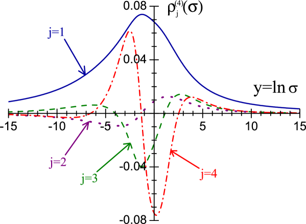
Figure 2: The four–loop spectral functions $\varrho^{(4)}_{j}(\sigma)$ (8): $\varrho^{(4)}_{1}(\sigma)$ (solid curve), $\varrho^{(4)}_{2}(\sigma)$ (dotted curve), $10\cdot\varrho^{(4)}_{3}(\sigma)$ (dashed curve), and $10^{2}\cdot\varrho^{(4)}_{4}(\sigma)$ (dot–dashed curve). The values of parameters: $n_{\mbox{\scriptsize f}}=3$, $y=\ln\sigma$.

First of all, it is convenient to express the spectral functions $\varrho^{(\ell)}_{j}(\sigma)$ (8) in terms of the real and imaginary parts of the $\ell$–loop couplant $a^{(\ell)}_{\mbox{\scriptsize s}}(Q^{2})$ on a physical cut:

$$\lim_{\varepsilon\to 0_{+}}a^{(\ell)}_{\mbox{\scriptsize s}}\Bigl{[}-\Lambda^{2}(\sigma\mp i\varepsilon)\Bigr{]}\equiv A^{(\ell)}_{\mbox{\scriptsize Re}}(\sigma)\mp i\pi A^{(\ell)}_{\mbox{\scriptsize Im}}(\sigma).$$ (13)

In this case Eq. (8) can be represented in a concise form:

$$\varrho^{(\ell)}_{j}(\sigma)=\sum_{k=0}^{K_{j}}{j\choose 2k+1}(-1)^{k}\,\pi^{2k}\Bigl{[}A^{(\ell)}_{\mbox{\scriptsize Im}}(\sigma)\Bigr{]}^{2k+1}\Bigl{[}A^{(\ell)}_{\mbox{\scriptsize Re}}(\sigma)\Bigr{]}^{j-2k-1},$$ (14)

where $K_{j}=j/2+(j\;\mbox{mod}\;2)/2-1$, and

$${n\choose m}=\frac{n!}{m!\,(n-m)!}$$ (15)

is the binomial coefficient. In particular, at any loop level

$$\varrho^{(\ell)}_{1}(\sigma) = A^{(\ell)}_{\mbox{\scriptsize Im}}(\sigma),$$ (16)

$$\varrho^{(\ell)}_{2}(\sigma) = 2A^{(\ell)}_{\mbox{\scriptsize Im}}(\sigma)A^{(\ell)}_{\mbox{\scriptsize Re}}(\sigma),$$ (17)

$$\varrho^{(\ell)}_{3}(\sigma) = A^{(\ell)}_{\mbox{\scriptsize Im}}(\sigma)\Biggl{\{}3\Bigl{[}A^{(\ell)}_{\mbox{\scriptsize Re}}(\sigma)\Bigr{]}^{2}-\pi^{2}\Bigl{[}A^{(\ell)}_{\mbox{\scriptsize Im}}(\sigma)\Bigr{]}^{2}\Biggr{\}},$$ (18)

$$\varrho^{(\ell)}_{4}(\sigma) = 4A^{(\ell)}_{\mbox{\scriptsize Im}}(\sigma)A^{(\ell)}_{\mbox{\scriptsize Re}}(\sigma)\Biggl{\{}\!\Bigl{[}A^{(\ell)}_{\mbox{\scriptsize Re}}(\sigma)\Bigr{]}^{2}-\pi^{2}\Bigl{[}A^{(\ell)}_{\mbox{\scriptsize Im}}(\sigma)\Bigr{]}^{2}\Biggr{\}}.\hskip 28.45274pt$$ (19)

Then, one has to calculate (by hands) the real and imaginary parts (13) of the couplants $a^{(\ell)}_{\mbox{\scriptsize s}}(Q^{2})$ (32)–(35) on a physical cut. In turn, this will enable one to construct the spectral functions $\varrho^{(\ell)}_{j}(\sigma)$ (14) corresponding to any integer power ($j\geq 1$) of the couplant $a^{(\ell)}_{\mbox{\scriptsize s}}(Q^{2})$ up to the four–loop level. The explicit expressions for the calculated functions $A^{(\ell)}_{\mbox{\scriptsize Im}}(\sigma)$ and $A^{(\ell)}_{\mbox{\scriptsize Re}}(\sigma)$ ($1\leq\ell\leq 4$) are given in App. B (see also App. C of Ref. [6] and App. C of Ref. [16]). The four–loop ($\ell=4$) spectral functions $\varrho^{(4)}_{j}(\sigma)$ ($1\leq j\leq 4$) are shown in Fig. 2.

4 Basic integrals

The explicit expressions for the spectral functions $\varrho^{(\ell)}_{j}(\sigma)$ (14) enable one to compute the corresponding nonpower expansion functions in spacelike (Eqs. (2) and (5)) and timelike (Eqs. (3) and (7)) domains. Specifically, in the framework of massless APT the spacelike expansion functions (2) read

$$\bar{A}_{\mbox{\tiny SL}}(z)=\int\limits_{0}^{\infty}\frac{\varrho(\sigma)}{\sigma+z}\,d\sigma.$$ (20)

For the numerical evaluation of $\bar{A}_{\mbox{\tiny SL}}(z)$ it is convenient to split Eq. (20) into three terms, namely

$$\bar{A}_{\mbox{\tiny SL}}(z)=\int\limits_{-1}^{0}\frac{r(x)e^{1/x}}{e^{1/x}+z}\,dx+\int\limits_{-1}^{1}\frac{\varrho_{y}(y)}{1+ze^{-y}}\,dy+\int\limits_{0}^{1}\frac{r(x)}{1+ze^{-1/x}}\,dx,$$ (21)

where

$$\varrho_{y}(y)=\varrho(\sigma)\biggr{|}_{\sigma=e^{y}},\qquad\varrho_{x}(x)=\varrho_{y}(y)\biggr{|}_{y=1/x},\qquad r(x)=\frac{\varrho_{x}(x)}{x^{2}}.$$ (22)

The numerical integration of Eq. (21) is implemented within QCDMAPT library by the subroutine APTSL (see Sect. 5). In turn, the timelike massless APT expansion functions (3) take the form

$$\bar{A}_{\mbox{\tiny TL}}(w)=\int\limits_{w}^{\infty}\varrho(\sigma)\,\frac{d\sigma}{\sigma}.$$ (23)

Similarly to the previous case, it is worth representing this equation in the following way:

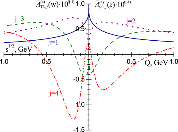
Figure 3: The four–loop “massless” APT expansion functions $\bar{A}^{(4)}_{\mbox{\tiny SL},\,j}(z)$ (2) and $\bar{A}^{(4)}_{\mbox{\tiny TL},\,j}(w)$ (3): $j=1$ (solid curves), $j=2$ (dotted curves, scaled$\,\times 10$), $j=3$ (dashed curves, scaled$\,\times 10^{2}$), and $j=4$ (dot–dashed curves, scaled$\,\times 10^{3}$). The values of parameters: $n_{\mbox{\scriptsize f}}=3$, $\Lambda=350\,$MeV, $z=Q^{2}/\Lambda^{2}$, $w=s/\Lambda^{2}$.

$$\bar{A}_{\mbox{\tiny TL}}(w)=\left\{\begin{array}[]{l}J_{1}\biggl{(}-1,\displaystyle{\frac{1}{\ln w}}\biggr{)}+J_{2}(-1,1)+J_{1}(0,1),\qquad\ln w<-1\\[12.80373pt] J_{2}(\ln w,1)+J_{1}(0,1),\qquad-1\leq\ln w<1\\[7.11317pt] J_{1}\biggl{(}0,\displaystyle{\frac{1}{\ln w}}\biggr{)},\qquad 1\leq\ln w\\ \end{array}\right.$$ (24)

where

$$J_{1}(x_{1},x_{2})=\int\limits_{x_{1}}^{x_{2}}r(x)\,dx,\qquad\quad J_{2}(y_{1},y_{2})=\int\limits_{y_{1}}^{y_{2}}\varrho_{y}(y)\,dy.$$ (25)

The numerical integration of Eq. (24) is implemented within QCDMAPT library by the subroutine APTTL (see Sect. 5). The four–loop massless APT expansion functions $\bar{A}^{(4)}_{\mbox{\tiny SL},\,j}(z)$ and $\bar{A}^{(4)}_{\mbox{\tiny TL},\,j}(w)$ ($1\leq j\leq 4$) are shown in Fig. 3.

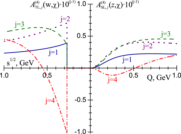
Figure 4: The four–loop MAPT expansion functions $A^{(4)}_{\mbox{\tiny SL},\,j}(z,\chi)$ (5) and $A^{(4)}_{\mbox{\tiny TL},\,j}(w,\chi)$ (7): $j=1$ (solid curves), $j=2$ (dotted curves, scaled$\,\times 10$), $j=3$ (dashed curves, scaled$\,\times 10^{2}$), and $j=4$ (dot–dashed curves, scaled$\,\times 10^{3}$). The values of parameters: $n_{\mbox{\scriptsize f}}=3$, $\Lambda=350\,$MeV, $m=270\,$MeV, $z=Q^{2}/\Lambda^{2}$, $w=s/\Lambda^{2}$.

In the framework of massive APT the spacelike expansion functions (5) read

$$A_{\mbox{\tiny SL}}(z,\chi)=\frac{z}{z+\chi}\int\limits_{\chi}^{\infty}\varrho(\sigma)\,\frac{\sigma-\chi}{\sigma+z}\,\frac{d\sigma}{\sigma}.$$ (26)

For the numerical evaluation of $A_{\mbox{\tiny SL}}(z,\chi)$ it is convenient to represent Eq. (26) in the following way:

$$A_{\mbox{\tiny SL}}(z,\chi)=\left\{\begin{array}[]{l}\!{\displaystyle\frac{z}{z+\chi}}\biggl{[}I_{1}\biggl{(}-1,\displaystyle{\frac{1}{\ln\chi}}\biggr{)}+\!I_{2}(-1,1)+I_{3}(0,1)\biggr{]},\qquad\ln\chi<-1\\[19.91692pt] \!{\displaystyle\frac{z}{z+\chi}}\Bigl{[}I_{2}(\ln\chi,1)+I_{3}(0,1)\Bigr{]},\qquad-1\leq\ln\chi<1\\[14.22636pt] \!{\displaystyle\frac{z}{z+\chi}}\,I_{3}\biggl{(}0,\displaystyle{\frac{1}{\ln\chi}}\biggr{)},\qquad 1\leq\ln\chi\\ \end{array}\right.$$ (27)

where

$$I_{1}(x_{1},x_{2})=\int\limits_{x_{1}}^{x_{2}}r(x)\,\frac{e^{1/x}-\chi}{e^{1/x}+z}\,dx,$$ (28)

$$I_{2}(y_{1},y_{2})=\int\limits_{y_{1}}^{y_{2}}\varrho_{y}(y)\,\frac{e^{y}-\chi}{e^{y}+z}\,dy,$$ (29)

$$I_{3}(x_{1},x_{2})=\int\limits_{x_{1}}^{x_{2}}r(x)\,\frac{1-\chi e^{-1/x}}{1+ze^{-1/x}}\,dx.$$ (30)

The numerical integration of Eq. (27) is implemented within QCDMAPT library by the subroutine MAPTSL (see Sect. 5). In turn, the timelike MAPT expansion functions (7) take the form

$$A_{\mbox{\tiny TL}}(w,\chi)=\theta(w-\chi)\int\limits_{w}^{\infty}\varrho(\sigma)\,\frac{d\sigma}{\sigma}=\theta(w-\chi)\bar{A}_{\mbox{\tiny TL}}(w),$$ (31)

where $\bar{A}_{\mbox{\tiny TL}}(w)$ is defined in Eq. (24). The numerical integration of Eq. (31) is implemented within QCDMAPT library by the subroutine MAPTTL (see Sect. 5). The four–loop MAPT expansion functions $A^{(4)}_{\mbox{\tiny SL},\,j}(z,\chi)$ and $A^{(4)}_{\mbox{\tiny TL},\,j}(w,\chi)$ ($1\leq j\leq 4$) are shown in Fig. 4.

5 Description of the template program

The provided template program (template.mw) is self–explaining. Besides, both template program and QCDMAPT library (QCDMAPT.lib) contain detailed comments.

The template program is organized as follows (see template.pdf). On the first page the QCDMAPT library is loaded and a sample set of input parameters is specified: $n_{\mbox{\scriptsize f}}=3$ active quarks, $Q=700\,$MeV, $s=(700\,\mbox{MeV})^{2}$, $m=270\,$MeV, and $\Lambda=350\,$MeV. The evaluation of expansion functions for the given set of parameters is presented on page 2. In particular, the first computation deals with the first–order ($j=1$) $\ell$–loop ($\ell=1,2,3,4$) expansion functions, namely, $a^{(\ell)}_{\mbox{\scriptsize s}}(Q^{2})$ (Eqs. (32)–(35)), $\bar{A}^{(\ell)}_{\mbox{\tiny SL},\,1}(z)$ (Eq. (2)), $\bar{A}^{(\ell)}_{\mbox{\tiny TL},\,1}(w)$ (Eq. (3)), $A^{(\ell)}_{\mbox{\tiny SL},\,1}(z,\chi)$ (Eq. (5)), and $A^{(\ell)}_{\mbox{\tiny TL},\,1}(w,\chi)$ (Eq. (7)). The second computation evaluates four–loop ($\ell=4$) expansion functions of $j$–th order ($j=1,2,3,4$), namely, $\bigl{[}a^{(4)}_{\mbox{\scriptsize s}}(Q^{2})\bigr{]}^{j}$ (Eq. (35)), $\bar{A}^{(4)}_{\mbox{\tiny SL},\,j}(z)$ (Eq. (2)), $\bar{A}^{(4)}_{\mbox{\tiny TL},\,j}(w)$ (Eq. (3)), $A^{(4)}_{\mbox{\tiny SL},\,j}(z,\chi)$ (Eq. (5)), and $A^{(4)}_{\mbox{\tiny TL},\,j}(w,\chi)$ (Eq. (7)). The data arrays of the first–order one–loop expansion functions are computed and relevant plots are presented on page 3 (see Fig. 1 and its caption for the details). The data arrays of the massless APT four–loop ($\ell=4$) expansion functions of $j$–th order ($j=1,2,3,4$) are computed and corresponding plots are presented on page 4 (see Fig. 3 and its caption for the details). The data arrays of the MAPT four–loop ($\ell=4$) expansion functions of $j$–th order ($j=1,2,3,4$) are computed and relevant plots are presented on page 5 (see Fig. 4 and its caption for the details).

The summary of QCDMAPT package commands is given below.

$\bullet\>$PERTURBATIVE QCD

AlphaPert$\,\ell\,$L(z) $=\alpha^{(\ell)}_{\mbox{\scriptsize s}}(Q^{2})$ ($\ell=1,2,3,4$; $z=Q^{2}/\Lambda^{2}$): $\ell$–loop perturbative strong running coupling, see App. A.

APert$\,\ell\,$L(z) $=a^{(\ell)}_{\mbox{\scriptsize s}}(Q^{2})=\alpha^{(\ell)}_{\mbox{\scriptsize s}}(Q^{2})\beta_{0}/(4\pi)$ ($\ell=1,2,3,4$; $z=Q^{2}/\Lambda^{2}$): $\ell$–loop perturbative QCD couplant, see Eqs. (32)–(35).

beta$\,j$ $=\beta_{j}$ ($j=0,1,2,3$): perturbative ($j+1$)–loop expansion coefficient of the QCD $\beta$ function, see Eqs. (36)–(39).

B$\,j$ $=B_{j}=\beta_{j}/\beta_{0}^{j+1}$ ($j=1,2,3$): combination of QCD $\beta$ function perturbative expansion coefficients, see App. A.

$\bullet\>$SPECTRAL FUNCTIONS

ARe$\,\ell\,$LY(y) $=A^{(\ell)}_{\mbox{\scriptsize Re}}(\sigma)\Bigr{|}_{\sigma=e^{y}}$ ($\ell=1,2,3,4$): real part of the $\ell$–loop perturbative QCD couplant on a physical cut, see Eqs. (13), (22), and App. B.

AIm$\,\ell\,$LY(y) $=A^{(\ell)}_{\mbox{\scriptsize Im}}(\sigma)\Bigr{|}_{\sigma=e^{y}}$ ($\ell=1,2,3,4$): imaginary part of the $\ell$–loop perturbative QCD couplant on a physical cut, see Eqs. (13), (22), and App. B.

Rho$\,\ell\,$L$\,j\,$pY(y) $=\varrho^{(\ell)}_{j}(\sigma)\Bigr{|}_{\sigma=e^{y}}$ ($\ell=1,2,3,4$; $j=1,...\,,\ell$): spectral function (in terms of $y=\ln\sigma$ variable) corresponding to $j$–th power of the $\ell$–loop perturbative QCD couplant, see Eqs. (8), (14), (22), and App. B.

R$\,\ell\,$L$\,j\,$pX(x) $=r_{j}^{(\ell)}(x)=x^{-2}\varrho^{(\ell)}_{j}(\sigma)\Bigr{|}_{\sigma=e^{1/x}}$ ($\ell=1,2,3,4$; $j=1,...\,,\ell$): spectral function (in terms of $x=1/\ln\sigma$ variable) corresponding to $j$–th power of the $\ell$–loop perturbative QCD couplant, see Eqs. (8), (14), (22), and App. B.

$\bullet\>$BASIC INTEGRALS

APTSL(RhoY,RX,z) $=\bar{A}_{\mbox{\tiny SL}}(z)$: numerical integration for the massless APT spacelike expansion functions, see Eqs. (20)–(22) with $\varrho_{y}(y)=\,$RhoY(y) and $r(x)=\,$RX(x).

APTTL(RhoY,RX,w) $=\bar{A}_{\mbox{\tiny TL}}(w)$: numerical integration for the massless APT timelike expansion functions, see Eqs. (23)–(25), (22) with $\varrho_{y}(y)=\,$RhoY(y) and $r(x)=\,$RX(x).

MAPTSL(RhoY,RX,z,chi) $=A_{\mbox{\tiny SL}}(z,\chi)$: numerical integration for the MAPT spacelike expansion functions, see Eqs. (26)–(30), (22) with $\varrho_{y}(y)=\,$RhoY(y) and $r(x)=\,$RX(x).

MAPTTL(RhoY,RX,w,chi) $=A_{\mbox{\tiny TL}}(w,\chi)$: numerical integration for the MAPT timelike expansion functions, see Eqs. (31), (23)–(25), (22) with $\varrho_{y}(y)=\,$RhoY(y) and $r(x)=\,$RX(x).

$\bullet\>$APT EXPANSION FUNCTIONS

ASL$\,\ell\,$L$\,j\,$p(z) $=\bar{A}^{(\ell)}_{\mbox{\tiny SL},\,j}(z)$ ($\ell=1,2,3,4$; $j=1,...\,,\ell$): APT spacelike expansion function ($\ell$–loop level, $j$–th order), see Eq. (2).

ATL$\,\ell\,$L$\,j\,$p(w) $=\bar{A}^{(\ell)}_{\mbox{\tiny TL},\,j}(w)$ ($\ell=1,2,3,4$; $j=1,...\,,\ell$): APT timelike expansion function ($\ell$–loop level, $j$–th order), see Eq. (3).

AlphaSL$\,\ell\,$L(z) $=\bar{A}^{(\ell)}_{\mbox{\tiny SL},\,1}(z)\,4\pi/\beta_{0}$ ($\ell=1,2,3,4$): APT spacelike $\ell$–loop effective coupling, see Eq. (2).

AlphaTL$\,\ell\,$L(w) $=\bar{A}^{(\ell)}_{\mbox{\tiny TL},\,1}(w)\,4\pi/\beta_{0}$ ($\ell=1,2,3,4$): APT timelike $\ell$–loop effective coupling, see Eq. (3).

$\bullet\>$MAPT EXPANSION FUNCTIONS

ASLm$\,\ell\,$L$\,j\,$p(z,chi) $=A^{(\ell)}_{\mbox{\tiny SL},\,j}(z,\chi)$ ($\ell=1,2,3,4$; $j=1,...\,,\ell$): MAPT spacelike expansion function ($\ell$–loop level, $j$–th order), see Eq. (5).

ATLm$\,\ell\,$L$\,j\,$p(w,chi) $=A^{(\ell)}_{\mbox{\tiny TL},\,j}(w,\chi)$ ($\ell=1,2,3,4$; $j=1,...\,,\ell$): MAPT timelike expansion function ($\ell$–loop level, $j$–th order), see Eq. (7).

AlphaSLm$\,\ell\,$L(z,chi) $=A^{(\ell)}_{\mbox{\tiny SL},\,1}(z,\chi)\,4\pi/\beta_{0}$ ($\ell=1,2,3,4$): MAPT spacelike $\ell$–loop effective coupling, see Eq. (5).

AlphaTLm$\,\ell\,$L(w,chi) $=A^{(\ell)}_{\mbox{\tiny TL},\,1}(w,\chi)\,4\pi/\beta_{0}$ ($\ell=1,2,3,4$): MAPT timelike $\ell$–loop effective coupling, see Eq. (7).

6 Conclusions

A program package, which facilitates computations in the framework of the Analytic approach to QCD, is developed. It includes the explicit expressions for relevant spectral functions calculated up to the four–loop level and the subroutines for necessary integrals.

This work was partially supported by the grants RFBR-08-01-00686, BRFBR-JINR-F08D-001, NS-1027.2008.2, and JINR grant.

Appendix A Perturbative QCD running coupling

This Section contains explicit expressions for the perturbative strong running coupling $\alpha^{(\ell)}_{\mbox{\scriptsize s}}(Q^{2})\equiv 4\pi\,a^{(\ell)}_{\mbox{\scriptsize s}}(Q^{2})/\beta_{0}$ up to the four–loop level. Specifically,

$$a^{(1)}_{\mbox{\scriptsize s}}(Q^{2}) = \frac{1}{\ln z},\qquad z=\frac{Q^{2}}{\Lambda^{2}},$$ (32)

$$a^{(2)}_{\mbox{\scriptsize s}}(Q^{2}) = \frac{1}{\ln z}-B_{1}\frac{\ln(\ln z)}{\ln^{2}z},$$ (33)

$$a^{(3)}_{\mbox{\scriptsize s}}(Q^{2}) = \frac{1}{\ln z}-B_{1}\frac{\ln(\ln z)}{\ln^{2}z}$$ (34)

$$+\frac{1}{\ln^{3}\!z}\biggl{\{}B_{1}^{2}\Bigl{[}\ln^{2}(\ln z)-\ln(\ln z)-1\Bigr{]}+B_{2}\biggr{\}},$$

$$a^{(4)}_{\mbox{\scriptsize s}}(Q^{2}) = \frac{1}{\ln z}-B_{1}\frac{\ln(\ln z)}{\ln^{2}z}$$ (35)

$$+\frac{1}{\ln^{3}\!z}\biggl{\{}B_{1}^{2}\Bigl{[}\ln^{2}(\ln z)-\ln(\ln z)-1\Bigr{]}+B_{2}\biggr{\}}$$

$$+\frac{1}{\ln^{4}\!z}\Biggl{\{}B_{1}^{3}\biggl{[}-\ln^{3}(\ln z)+\frac{5}{2}\ln^{2}(\ln z)$$

$$+2\ln(\ln z)-\frac{1}{2}\biggr{]}-3B_{1}B_{2}\ln(\ln z)+\frac{1}{2}B_{3}\Biggr{\}},\hskip 14.22636pt$$

where $B_{j}=\beta_{j}/\beta_{0}^{j+1}$ is the combination of QCD $\beta$ function perturbative expansion coefficients:

$$\beta_{0} = 11-\frac{2}{3}n_{\mbox{\scriptsize f}},$$ (36)

$$\beta_{1} = 102-\frac{38}{3}n_{\mbox{\scriptsize f}},$$ (37)

$$\beta_{2} = \frac{2857}{2}-\frac{5033}{18}n_{\mbox{\scriptsize f}}+\frac{325}{54}n_{\mbox{\scriptsize f}}^{2},$$ (38)

$$\beta_{3} = \frac{149753}{6}+3564\zeta(3)-\left[\frac{1078361}{162}+\frac{6508}{27}\zeta(3)\right]\!n_{\mbox{\scriptsize f}}$$ (39)

$$+\left[\frac{50065}{162}+\frac{6472}{81}\zeta(3)\right]\!n_{\mbox{\scriptsize f}}^{2}+\frac{1093}{729}n_{\mbox{\scriptsize f}}^{3}.$$

In these equations $n_{\mbox{\scriptsize f}}$ stands for the number of active quarks and $\zeta(x)$ denotes the Riemann $\zeta$ function, $\zeta(3)\simeq 1.202$. The one– and two–loop coefficients ($\beta_{0}$ and $\beta_{1}$) are scheme–independent, whereas the expressions given for $\beta_{2}$ and $\beta_{3}$ are calculated in the $\overline{\mbox{MS}}$ subtraction scheme (see papers [22, 23, 24, 25] and references therein for the details). Note that expressions (33)–(35) correspond to approximate solutions of the perturbative renormalization group (RG) equation for the QCD invariant charge, see, e.g., Ref. [26], Sect. 2 of review [15], and App. A of review [16]. Nonetheless, the difference between the approximate running coupling $\alpha^{(\ell)}_{\mbox{\scriptsize s}}(Q^{2})$ (33)–(35) and the exact solution of perturbative RG equation $\alpha^{(\ell)}_{\mbox{\scriptsize ex}}(Q^{2})$ is not controllable at every considered loop level.

Appendix B Spectral functions

As it has been mentioned in Sect. 3, the spectral functions $\varrho^{(\ell)}_{j}(\sigma)$ (8) can be represented in the following form:

$$\varrho^{(\ell)}_{j}(\sigma)=\sum_{k=0}^{K_{j}}{j\choose 2k+1}(-1)^{k}\,\pi^{2k}\Bigl{[}A^{(\ell)}_{\mbox{\scriptsize Im}}(\sigma)\Bigr{]}^{2k+1}\Bigl{[}A^{(\ell)}_{\mbox{\scriptsize Re}}(\sigma)\Bigr{]}^{j-2k-1},$$ (40)

where

$$\lim_{\varepsilon\to 0_{+}}a^{(\ell)}_{\mbox{\scriptsize s}}\Bigl{[}-\Lambda^{2}(\sigma\mp i\varepsilon)\Bigr{]}\equiv A^{(\ell)}_{\mbox{\scriptsize Re}}(\sigma)\mp i\pi A^{(\ell)}_{\mbox{\scriptsize Im}}(\sigma),$$ (41)

$\ell$–loop perturbative couplants $a^{(\ell)}_{\mbox{\scriptsize s}}(Q^{2})$ are given by Eqs. (32)–(35), and $K_{j}=j/2+(j\;\mbox{mod}\;2)/2-1$. The functions $A^{(\ell)}_{\mbox{\scriptsize Im}}(\sigma)$ and $A^{(\ell)}_{\mbox{\scriptsize Re}}(\sigma)$, calculated up to the four–loop level ($1\leq\ell\leq 4$), are listed below.

One–loop level:

$$A^{(1)}_{\mbox{\scriptsize Im}}(\sigma)=\frac{1}{y^{2}+\pi^{2}},\qquad\quad A^{(1)}_{\mbox{\scriptsize Re}}(\sigma)=\frac{y}{y^{2}+\pi^{2}},\qquad\quad y=\ln\sigma.$$ (42)

Two–loop level:

$$A^{(2)}_{\mbox{\scriptsize Im}}(\sigma) = \frac{1}{(y^{2}+\pi^{2})^{2}}\Bigl{[}2yS^{(2)}_{\mbox{\scriptsize 1}}(y)+(\pi^{2}-y^{2})S^{(2)}_{\mbox{\scriptsize 2}}(y)\Bigr{]},$$ (43)

$$A^{(2)}_{\mbox{\scriptsize Re}}(\sigma) = \frac{1}{(y^{2}+\pi^{2})^{2}}\Bigl{[}(y^{2}-\pi^{2})S^{(2)}_{\mbox{\scriptsize 1}}(y)+2\pi^{2}yS^{(2)}_{\mbox{\scriptsize 2}}(y)\Bigr{]},$$ (44)

where

$$S^{(2)}_{\mbox{\scriptsize 1}}(y) = y-\frac{B_{1}}{2}\ln(y^{2}+\pi^{2}),$$ (45)

$$S^{(2)}_{\mbox{\scriptsize 2}}(y) = 1-B_{1}\biggl{[}\frac{1}{2}-\frac{1}{\pi}\arctan\!\left(\frac{y}{\pi}\right)\biggr{]}\!,$$ (46)

and $B_{j}=\beta_{j}/\beta_{0}^{j+1}$ is the combination of QCD $\beta$ function perturbative expansion coefficients (see App. A).

Three–loop level:

$$A^{(3)}_{\mbox{\scriptsize Im}}(\sigma) = \frac{1}{(y^{2}+\pi^{2})^{3}}\Bigl{[}(3y^{2}-\pi^{2})S^{(3)}_{\mbox{\scriptsize 3}}(y)-y(y^{2}-3\pi^{2})S^{(3)}_{\mbox{\scriptsize 4}}(y)\Bigr{]}\!,$$ (47)

$$A^{(3)}_{\mbox{\scriptsize Re}}(\sigma) = \frac{1}{(y^{2}+\pi^{2})^{3}}\Bigl{[}y(y^{2}-3\pi^{2})S^{(3)}_{\mbox{\scriptsize 3}}(y)+\pi^{2}(3y^{2}-\pi^{2})S^{(3)}_{\mbox{\scriptsize 4}}(y)\Bigr{]}\!,\hskip 42.67912pt$$ (48)

where

$$S^{(3)}_{\mbox{\scriptsize 1}}(y) = \frac{1}{2}\ln(y^{2}+\pi^{2}),$$ (49)

$$S^{(3)}_{\mbox{\scriptsize 2}}(y) = \frac{1}{2}-\frac{1}{\pi}\arctan\!\left(\frac{y}{\pi}\right),$$ (50)

$$S^{(3)}_{\mbox{\scriptsize 3}}(y) = y^{2}-\pi^{2}-B_{1}\!\left[yS^{(3)}_{\mbox{\scriptsize 1}}(y)-\pi^{2}S^{(3)}_{\mbox{\scriptsize 2}}(y)\right]$$ (51)

$$+B_{1}^{2}\biggl{\{}\!S^{(3)}_{\mbox{\scriptsize 1}}(y)\!\left[S^{(3)}_{\mbox{\scriptsize 1}}(y)-1\right]-\pi^{2}\!\left[S^{(3)}_{\mbox{\scriptsize 2}}(y)\right]^{2}-1\!\biggr{\}}+B_{2},$$

$$S^{(3)}_{\mbox{\scriptsize 4}}(y) = 2y-B_{1}\!\left[S^{(3)}_{\mbox{\scriptsize 1}}(y)+yS^{(3)}_{\mbox{\scriptsize 2}}(y)\right]\!+B_{1}^{2}S^{(3)}_{\mbox{\scriptsize 2}}(y)\!\left[2S^{(3)}_{\mbox{\scriptsize 1}}(y)-1\right].\hskip 42.67912pt$$ (52)

Four–loop level:

$$A^{(4)}_{\mbox{\scriptsize Im}}(\sigma) = \frac{1}{(y^{2}+\pi^{2})^{4}}\biggl{\{}\!4y(y^{2}-\pi^{2})\!\left[S^{(4)}_{\mbox{\scriptsize 3}}(y)+S^{(4)}_{\mbox{\scriptsize 5}}(y)+S^{(4)}_{\mbox{\scriptsize 7}}(y)\right]$$ (53)

$$+\Bigl{[}4\pi^{2}y^{2}-(y^{2}-\pi^{2})^{2}\Bigr{]}\!\Bigl{[}S^{(4)}_{\mbox{\scriptsize 4}}(y)+S^{(4)}_{\mbox{\scriptsize 6}}(y)+S^{(4)}_{\mbox{\scriptsize 8}}(y)\Bigr{]}\!\biggr{\}}\!,$$

$$A^{(4)}_{\mbox{\scriptsize Re}}(\sigma) = \frac{1}{(y^{2}+\pi^{2})^{4}}\biggl{\{}\!\Bigl{[}(y^{2}-\pi^{2})^{2}-4\pi^{2}y^{2}\Bigr{]}\!\Bigl{[}S^{(4)}_{\mbox{\scriptsize 3}}(y)+S^{(4)}_{\mbox{\scriptsize 5}}(y)+S^{(4)}_{\mbox{\scriptsize 7}}(y)\Bigr{]}$$ (54)

$$+4\pi^{2}y(y^{2}-\pi^{2})\!\left[S^{(4)}_{\mbox{\scriptsize 4}}(y)+S^{(4)}_{\mbox{\scriptsize 6}}(y)+S^{(4)}_{\mbox{\scriptsize 8}}(y)\right]\!\biggr{\}}\!,\hskip 14.22636pt$$

where

$$S^{(4)}_{\mbox{\scriptsize 1}}(y) = \frac{1}{2}\ln(y^{2}+\pi^{2}),$$ (55)

$$S^{(4)}_{\mbox{\scriptsize 2}}(y) = \frac{1}{2}-\frac{1}{\pi}\arctan\!\left(\frac{y}{\pi}\right)\!,$$ (56)

$$S^{(4)}_{\mbox{\scriptsize 3}}(y) = B_{1}^{2}\,y\biggl{\{}\!S^{(4)}_{\mbox{\scriptsize 1}}(y)\!\left[S^{(4)}_{\mbox{\scriptsize 1}}(y)-1\right]-\pi^{2}\!\left[S^{(4)}_{\mbox{\scriptsize 2}}(y)\right]^{2}+\frac{B_{2}}{B_{1}^{2}}-1\!\biggr{\}}\hskip 28.45274pt$$ (57)

$$-B_{1}^{2}\,\pi^{2}S^{(4)}_{\mbox{\scriptsize 2}}(y)\!\left[2S^{(4)}_{\mbox{\scriptsize 1}}(y)-1\right]\!,$$

$$S^{(4)}_{\mbox{\scriptsize 4}}(y) = B_{1}^{2}\biggl{\{}\!S^{(4)}_{\mbox{\scriptsize 1}}(y)\!\left[S^{(4)}_{\mbox{\scriptsize 1}}(y)-1\right]-\pi^{2}\!\left[S^{(4)}_{\mbox{\scriptsize 2}}(y)\right]^{2}$$ (58)

$$+\,y\,S^{(4)}_{\mbox{\scriptsize 2}}(y)\!\left[2S^{(4)}_{\mbox{\scriptsize 1}}(y)-1\right]+\frac{B_{2}}{B_{1}^{2}}-1\biggr{\}}\!,$$

$$S^{(4)}_{\mbox{\scriptsize 5}}(y) = B_{1}^{3}\Biggl{\{}\!S^{(4)}_{\mbox{\scriptsize 1}}(y)\!\left[3\pi^{2}\!\left(S^{(4)}_{\mbox{\scriptsize 2}}(y)\right)^{2}-\left(S^{(4)}_{\mbox{\scriptsize 1}}(y)\right)^{2}\right]$$ (59)

$$+\,\frac{5}{2}\left[\left(S^{(4)}_{\mbox{\scriptsize 1}}(y)\right)^{2}-\pi^{2}\left(S^{(4)}_{\mbox{\scriptsize 2}}(y)\right)^{2}\right]$$

$$+\,S^{(4)}_{\mbox{\scriptsize 1}}(y)\!\left(2-3\,\frac{B_{2}}{B_{1}^{2}}\right)+\frac{1}{2}\!\left(\frac{B_{3}}{B_{1}^{3}}-1\right)\!\Biggr{\}}\!,$$

$$S^{(4)}_{\mbox{\scriptsize 6}}(y) = B_{1}^{3}S^{(4)}_{\mbox{\scriptsize 2}}(y)\biggl{\{}\!\pi^{2}\!\left[S^{(4)}_{\mbox{\scriptsize 2}}(y)\right]^{2}-3\!\left[S^{(4)}_{\mbox{\scriptsize 1}}(y)\right]^{2}$$ (60)

$$+\,5S^{(4)}_{\mbox{\scriptsize 1}}(y)-3\frac{B_{2}}{B_{1}^{2}}+2\biggr{\}}\!,$$

$$S^{(4)}_{\mbox{\scriptsize 7}}(y) = y(y^{2}-3\pi^{2})+B_{1}\Bigl{[}2\pi^{2}yS^{(4)}_{\mbox{\scriptsize 2}}(y)-(y^{2}-\pi^{2})S^{(4)}_{\mbox{\scriptsize 1}}(y)\Bigr{]}\!,\hskip 28.45274pt$$ (61)

$$S^{(4)}_{\mbox{\scriptsize 8}}(y) = 3y^{2}-\pi^{2}-B_{1}\Bigl{[}(y^{2}-\pi^{2})S^{(4)}_{\mbox{\scriptsize 2}}(y)+2yS^{(4)}_{\mbox{\scriptsize 1}}(y)\Bigr{]}\!.$$ (62)

References

- [1] D.V. Shirkov and I.L. Solovtsov, Phys. Rev. Lett. 79, 1209 (1997).
- [2] K.A. Milton and I.L. Solovtsov, Phys. Rev. D 55, 5295 (1997); 59, 107701 (1999).
- [3] D.V. Shirkov and I.L. Solovtsov, Theor. Math. Phys. 120, 1220 (1999); 150, 132 (2007).
- [4] M. Baldicchi and G.M. Prosperi, Phys. Rev. D 66, 074008 (2002); AIP Conf. Proc. 756, 152 (2005).
- [5] M. Baldicchi, A.V. Nesterenko, G.M. Prosperi, D.V. Shirkov, and C. Simolo, Phys. Rev. Lett. 99, 242001 (2007).
- [6] M. Baldicchi, A.V. Nesterenko, G.M. Prosperi, and C. Simolo, Phys. Rev. D 77, 034013 (2008).
- [7] A.V. Nesterenko, Phys. Rev. D 62, 094028 (2000); 64, 116009 (2001).
- [8] A.C. Aguilar, A.V. Nesterenko, and J. Papavassiliou, J. Phys. G 31, 997 (2005); Nucl. Phys. B (Proc. Suppl.) 164, 300 (2007).
- [9] K.A. Milton, I.L. Solovtsov, and O.P. Solovtsova, Phys. Lett. B 439, 421 (1998); Phys. Rev. D 60, 016001 (1999); R.S. Pasechnik, D.V. Shirkov, and O.V. Teryaev, ibid. 78, 071902 (2008).
- [10] A.P. Bakulev, K. Passek–Kumericki, W. Schroers, and N.G. Stefanis, Phys. Rev. D 70, 033014 (2004); 70, 079906(E) (2004); A.P. Bakulev, A.V. Pimikov, and N.G. Stefanis, ibid. 79, 093010 (2009).
- [11] A.P. Bakulev, S.V. Mikhailov, and N.G. Stefanis, Phys. Rev. D 72, 074014 (2005); 72, 119908(E) (2005); 75, 056005 (2007); 77, 079901(E) (2008).
- [12] A.V. Kotikov, A.V. Lipatov, and N.P. Zotov, J. Exp. Theor. Phys. 101, 811 (2005); G. Cvetic, A.Y. Illarionov, B.A. Kniehl, and A.V. Kotikov, Phys. Lett. B 679, 350 (2009); A.Y. Illarionov and A.V. Kotikov, arXiv:0912.4355 [hep-ph].
- [13] A.I. Alekseev and B.A. Arbuzov, Phys. Atom. Nucl. 61, 264 (1998); Mod. Phys. Lett. A 13, 1747 (1998); 20, 103 (2005).
- [14] G. Cvetic and C. Valenzuela, J. Phys. G 32, L27 (2006); Phys. Rev. D 74, 114030 (2006); 77, 074021 (2008); Braz. J. Phys. 38, 371 (2008); G. Cvetic and H.E. Martinez, J. Phys. G 36, 125006 (2009); G. Cvetic, R. Koegerler, and C. Valenzuela, arXiv:0912.2466 [hep-ph].
- [15] G.M. Prosperi, M. Raciti, and C. Simolo, Prog. Part. Nucl. Phys. 58, 387 (2007).
- [16] A.V. Nesterenko, Int. J. Mod. Phys. A 18, 5475 (2003).
- [17] A.V. Nesterenko and J. Papavassiliou, J. Phys. G 32, 1025 (2006).
- [18] A.V. Nesterenko, Nucl. Phys. B (Proc. Suppl.) 186, 207 (2009); SLAC eConf C0706044, 25 (2008).
- [19] S.L. Adler, Phys. Rev. D 10, 3714 (1974); A. De Rujula and H. Georgi, ibid. 13, 1296 (1976).
- [20] A.V. Nesterenko and I.L. Solovtsov, Mod. Phys. Lett. A 16, 2517 (2001).
- [21] D.V. Shirkov and A.V. Zayakin, Phys. Atom. Nucl. 70, 775 (2007).
- [22] D.J. Gross and F. Wilczek, Phys. Rev. Lett. 30, 1343 (1973); H.D. Politzer, ibid. 30, 1346 (1973).
- [23] W.E. Caswell, Phys. Rev. Lett. 33, 244 (1974); D.R.T. Jones, Nucl. Phys. B 75, 531 (1974); E. Egorian and O.V. Tarasov, Theor. Math. Phys. 41, 863 (1979).
- [24] O.V. Tarasov, A.A. Vladimirov, and A.Yu. Zharkov, Phys. Lett. B 93, 429 (1980); S.A. Larin and J.A.M. Vermaseren, ibid. 303, 334 (1993).
- [25] T. van Ritbergen, J.A.M. Vermaseren, and S.A. Larin, Phys. Lett. B 400, 379 (1997); K.G. Chetyrkin, B.A. Kniehl, and M. Steinhauser, Phys. Rev. Lett. 79, 2184 (1997).
- [26] E. Gardi, G. Grunberg, and M. Karliner, JHEP 9807, 007 (1998); B.A. Magradze, arXiv:hep-ph/9808247; arXiv:hep-ph/0305020.