Anomalous diffusion in disordered multi-channel systems

Abstract

We study diffusion of a particle in a system composed of $K$ parallel channels, where the transition rates within the channels are quenched random variables whereas the inter-channel transition rate $v$ is homogeneous. A variant of the strong disorder renormalization group method and Monte Carlo simulations are used. Generally, we observe anomalous diffusion, where the average distance travelled by the particle, $[\langle x(t)\rangle]_{\rm av}$, has a power-law time-dependence $[\langle x(t)\rangle]_{\rm av}\sim t^{\mu_{K}(v)}$, with a diffusion exponent $0\leq\mu_{K}(v)\leq 1$. In the presence of left-right symmetry of the distribution of random rates the recurrent point of the multi-channel system is independent of $K$, and the diffusion exponent is found to increase with $K$ and decrease with $v$. In the absence of this symmetry, the recurrent point may be shifted with $K$ and the current can be reversed by varying the lane change rate $v$.

1 Introduction

Brownian motion is one of the most studied and the best understood stochastic processes, both in homogeneous and in random environments [1, 2, 3, 4]. Physical motivation to study diffusion in disordered media is provided by transport processes (molecular diffusion, electric conduction, biological transport in a cell) on the one hand and by relaxation in complex systems (in spin glasses and random ferromagnets) on the other. For asymmetric hoppings, when the microscopic transition rates depend on the direction, too, disorder can strongly modify the properties of the transport in dimensions, $d<2$ [4].

The effect of disorder is particularly strong in $1d$, in which case several exact results are known [5, 6, 7, 8, 9, 10]. Many of those are obtained in a mathematically rigorous way, such as Sinai-scaling of the average square displacement, $[\langle x^{2}(t)\rangle]_{\rm av}$ in time, $t$ [7]. This behaves at the recurrent point as:

$$[\langle x^{2}(t)\rangle]_{\rm av}\sim\ln^{4}(t)\;,$$ (1)

where $\langle\dots\rangle$ stands for the thermal average for a given realization of disorder and $[\dots]_{\rm av}$ is used to denote averaging over quenched disorder. Some presumably exact results are also calculated by a physically motivated method using a strong disorder renormalization group approach [11]. In this method sites of the lattice having the smallest barrier in the random potential landscape are consecutively eliminated and new transition rates are perturbatively calculated between remaining sites. Thus during renormalization the fastest rates are eliminated and at the fixed point only the slow excitations remain, which govern the cooperative dynamics of the system. The fixed point of the transformation is a so called infinite disorder fixed point, at which the ratio of transition rates between neighbouring sites goes either to zero or to infinity, so that the transformation becomes asymptotically exact. The infinite disorder fixed point of the $1d$ random random walk is isomorphic with the fixed point of some $1d$ random quantum magnets[12], such as the random transverse-field Ising spin chain[13] and some critical properties of the two models are interrelated [14].

It is convenient to introduce a control parameter of the random random walk, $\delta$, which has the value $\delta=0$ at the recurrent point, which corresponds to the fixed point of the strong disorder renormalization group transformation. In the recurrent point the correlation length of the system is divergent. On the contrary for $\delta\neq 0$ when the walk is drifted to one or another direction the correlation length is finite and this regime is called the transient phase. In the transient phase the average travelled distance, $[\langle x(t)\rangle]_{\rm av}$, is non-zero and has a power-low time-dependence:

$$[\langle x(t)\rangle]_{\rm av}\sim t^{\mu_{1}}\;,$$ (2)

where the diffusion exponent, $\mu_{1}=\mu_{1}(\delta)\leq 1$, is a continuous function of the control parameter. According to renormalization group analysis in the vicinity of the critical point it behaves as[11, 14]:

$$\mu_{1}(\delta)=\delta+O(\delta^{2})\;.$$ (3)

In reality, the channel in which the transport takes place is often not strictly one-dimensional. For example, we may think of vehicular traffic in multi-lane roads [15] or the active transport in cells, which is realized by molecular motors moving on filaments that are composed of several proto-filaments [16]. Besides, the problem of one dimensional random walks with long (but bounded) jump lengths is also equivalent to random walks with nearest neighbour jumps in a strip of finite width. This problem arises also in the context of disordered iterated maps [18] or for random walks with inertia [19]. Comparatively, less results are known for random walks on strips [17, 20], which can be considered to be in a way between dimensions one and two. Only very recently, it has been shown that at the recurrent point of the multi-channel system, Sinai scaling in Eq.(1) is valid [21]. The same conclusion is obtained by one of us by using a variant of the strong disorder renormalization group method [22]. Indeed, during renormalization the strip is renormalized to a random chain, thus results quoted above in Eqs. (2) and (3) are expected to hold in this case, too.

In this work we are going to study the properties of a random walk in a disordered multi-channel system, we pay particular attention to the transient phase. In this study we consider systems composed of $K$ channels with quenched random transition rates within channels and allow symmetric transitions between channels with a site-independent lane change rate $v$. We measure the diffusion exponent in the system, $\mu_{K}(v)$, and study its dependence on $K$ and $v$. In the strong coupling limit, $v\to\infty$, and in the vicinity of the recurrent point we obtain analytical results. In the general situation we use numerical methods, either Monte-Carlo simulations or numerical application of the strong disorder renormalization group method.

The rest of the paper is organized as follows. The model is presented in Sec. 2 and its properties are analyzed in the strong coupling limit in Sec.3. The essence of the renormalization procedure and phenomenological scaling considerations are given in Sec.4. Numerical analysis for $K=2$ and for varying lane change rate is given in Sec.5. Our results are discussed in the final Section.

2 Model

2.1 $1d$ systems

We define the model first in one-dimension, on the discrete points, $l=1,2,\dots,L$, with periodic boundaries. A continuous time stochastic process is considered in which the particle jumps from site $l$ to site $l+1$ with a transition rate, $p_{l}$, which may be different from the transition rate of the reverse jump, $(l+1\to l)$, denoted by $q_{l+1}$. Here the pairs of rates ($p_{l}$,$q_{l}$) are independent and identically distributed random variables drawn from the distribution $P(p,q)$. We generally consider the limit $L\to\infty$ and are interested in the asymptotic (long time) behavior.

The control parameter of the $1d$ random walk is defined as[11, 14]:

$$\delta=\frac{[\ln p]_{\rm av}-[\ln q]_{\rm av}}{{\rm var}[\ln p]+{\rm var}[\ln q]}\;,$$ (4)

where ${\rm var}[y]$ stands for the variance of $y$. In the $1d$ problem, the mean velocity and the diffusion constant of a particle on a finite ring is expressed as a Kesten random variable and therefore the diffusion exponent, $\mu_{1}$, can be calculated exactly even for not small $\delta$ [5, 6, 9]. It is given by the positive root of the equation:

$$\left[\left(\frac{q}{p}\right)^{\mu_{1}}\right]_{\rm av}=1,$$ (5)

provided it is smaller than one. Otherwise the particle moves with a finite mean velocity and $\mu_{1}=1$. Indeed for small $\delta$ Eq(5) gives back the leading behavior of the renormalization group result in Eq.(3).

In this paper we consider two types of random environments. For type A (or symmetric) randomness the transition rates satisfy the relation that the product, $p_{l}q_{l}$, does not depend on the position and the distribution of the rates is symmetric at the recurrent point, i.e. $P(p,q)=P(q,p)$. Here we use a bimodal disorder:

$$p_{l}=\frac{1}{q_{l}}=\left\{\begin{array}[]{c}{\lambda\qquad{\rm with~{}probability}~{}c,}\\ {1/\lambda\qquad{\rm with~{}probability}~{}1-c,}\end{array}\right.$$ (6)

for which the control parameter is given by:

$$\delta_{A}=\frac{2c-1}{4c(1-c)}\frac{1}{\ln\lambda}\;,$$ (7)

and the diffusion exponent is:

$$\mu_{1}(A)=\left|\frac{\ln(c^{-1}-1)}{2\ln\lambda}\right|\;.$$ (8)

For type B (or asymmetric) randomness the distribution of rates is non-symmetric at the recurrent point either. We have used the following distribution:

$$p_{l}=1,\quad q_{l}=\left\{\begin{array}[]{c}{\lambda\qquad{\rm with~{}probability}~{}c,}\\ {1/\lambda\qquad{\rm with~{}probability}~{}1-c,}\end{array}\right.$$ (9)

the control parameter is given by:

$$\delta_{B}=-\frac{2c-1}{4c(1-c)}\frac{1}{\ln\lambda}\;,$$ (10)

and the diffusion exponent is:

$$\mu_{1}(B)=\left|\frac{\ln(c^{-1}-1)}{\ln\lambda}\right|\;.$$ (11)

2.2 Multi-channel systems

The multi-channel system consists of $i=1,2,\dots,K$ channels in which the transition rates are drawn independently from each other but from the same distribution $P(p,q)$. Lane changes occur with rate $v$ between nearest neighbor lanes (also between lane $i=K$ and $i=1$), which does not depend on the position. This means that the transition rate, $w[(l,i)\to(k,j)]$, for a jump from site $(l,i)$ to site $(k,j)$ is given by:

$$w[(l,i)\to(k,j)]=\delta_{i,j}\left(p^{(i)}_{l}\delta_{l+1,k}+q^{(i)}_{l}\delta_{l,k}\right)+\delta_{l,k}\left(\delta_{i+1,j}+\delta_{i-1,j}\right)v\;.$$ (12)

Similarly to the one dimensional model, the multi-channel system has a recurrent point at, otherwise it is transient in the positive or negative directions. The transient regions consist of two phases: in the sublinear transient phase $\mu_{K}<1$, while in the ballistic phase $\mu_{K}=1$.

For symmetric randomness, it is easy to see that the recurrent point is not shifted for $K>1$ compared to that of $K=1$. It is due to the fact that here recurrence is connected with the left-right symmetry of the distribution of the transition rates, which stays invariant after connecting the channels, too. On the contrary, for asymmetric randomness, the condition of recurrence depends on $K$ and $v$.

3 Strong-coupling limit

First, we discuss the strong coupling limit ($v\to\infty$), which is simple enough to obtain analytical results. In the following, the set of $K$ sites with the horizontal coordinate $l$ will be called the $l$th layer. In the limit $v\to\infty$, the particle being in the $l$th layer, visits all sites of the layer infinitely many times before jumping to another layer. Consequently, the effective transition rate between layers is just the average of the interlayer jump rates over the vertical coordinate:

$$\tilde{p}_{l}=\frac{\sum_{i}p^{(i)}_{l}}{K},\quad\tilde{q}_{l}=\frac{\sum_{i}q^{(i)}_{l}}{K}\;,$$ (13)

and the problem is reduced to an effective one-dimensional random walk. The corresponding $1d$ random environment is given by the transition rates, $\tilde{p}_{l}$ and $\tilde{q}_{l}$, the distributions of which follow from the distributions of the original chain, respectively. In the following we analyse the properties of the strong coupling limit for the two different types of randomness.

3.1 Symmetric randomness

Let us consider a general symmetric randomness, where $p^{(i)}_{l}q^{(i)}_{l}=1$ at all $(l,i)$ sites and the probability density of $p^{(i)}_{l}$ is denoted by $\rho(p)$. As we have already mentioned, if $\delta_{A}=0$ then the system is recurrent for any $K>1$, due to the symmetry of the distribution $P(p,q)$.

Specially for $K=2$, the diffusion exponent $\mu_{2}$ can be given in terms of $\mu_{1}$ as follows. For the effective one-channel system with rates given in Eq. (13)), equation (5) can be written as:

$$\int{\rm d}p_{1}\rho(p_{1})\int{\rm d}p_{2}\rho(p_{2})\left(\frac{1/p_{1}+1/p_{2}}{p_{1}+p_{2}}\right)^{\mu_{2}}=$$

$$\int{\rm d}p_{1}\rho(p_{1})(p_{1})^{-\mu_{2}}\int{\rm d}p_{2}\rho(p_{2})(p_{2})^{-\mu_{2}}.$$ (14)

The diffusion exponent $\mu_{1}$ for the case $K=1$ is determined by

$$\int{\rm d}p\rho(p)(p)^{-2\mu_{1}}=1\;.$$ (15)

Comparing the latter two equations, we obtain the simple relation:

$$\mu_{2}=2\mu_{1},\quad v\to\infty\;.$$ (16)

For $K>2$ a similar relation holds only for weak disorder and in the vicinity of the recurrent point. Here for weak disorder we use the parametrization $p_{l}=1+\epsilon_{l}$, with $|\epsilon_{l}|\ll 1$ in which case in the $K$-channel system the control parameter, $\delta_{A}^{(K)}$ is simply related to the control parameter in the one lane system, $\delta_{A}$, as $\delta_{A}^{(K)}\simeq K\delta_{A}$. Consequently one obtains for the diffusion exponent from eq.(3):

$$\mu_{K}\simeq K\mu_{1},\quad\mu_{1}\ll 1\quad{\rm and}\quad v\to\infty\;.$$ (17)

Thus with increasing number of channels, the extension of the sub-linear transient regime, measured by $\delta_{A}$ is decreasing and, for any fixed $\delta_{A}>0$ and sufficiently large $K$, the transport becomes ballistic.

For large values of $K$ the effective transition rates in Eq.(13) will approach a Gaussian distribution with a relative mean deviation, which is decreasing with $K$. Consequently the disorder of the effective couplings will be weak for large $K$, thus one expects that $\mu_{K}/K\to const$. We have checked this expectation by using the bimodal distribution in Eq.(6), when for general $K$, the diffusion exponent has been obtained by solving numerically the equation:

$$\sum_{n=0}^{K}\frac{K!}{n!(K-n)!}c^{K-n}(1-c)^{n}\left(\frac{n\lambda^{2}+K-n}{n+(K-n)\lambda^{2}}\right)^{\mu_{K}}=1\;.$$ (18)

The obtained values of $\mu_{K}$ for different number of channels are shown in Fig.1 for two different bimodal parameters.

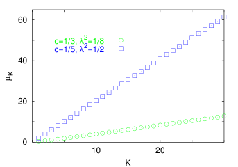
Figure 1: Diffusion exponent, $\mu_{K}$, plotted against the number of channels, $K$, in the large coupling limit for symmetric randomness in Eq.(6) calculated from Eq.(18).

Indeed, $\mu_{K}$ is found to be approximately linear in $K$ for large $K$ in both cases.

3.2 Asymmetric randomness

Next, we consider the bimodal disorder in Eq.(9). The probability $c=c^{*}_{K}$ for which the system is recurrent is the root of the following equation:

$$\sum_{n=0}^{K}\frac{K!}{n!(K-n)!}(c^{*}_{K})^{K-n}(1-c^{*}_{K})^{n}\ln\frac{(K-n)\lambda+n\lambda^{-1}}{K}=0\;.$$ (19)

For $K=2$ it is explicitly given as:

$$c^{*}_{2}(\lambda)=\frac{1}{2}(1+f-\sqrt{1+f^{2}}),\quad f=\ln\lambda/\ln[(\lambda+\lambda^{-1})/2]\;.$$ (20)

For weak disorder we have $\lim_{\lambda\to 1}c^{*}_{2}(\lambda)=c^{*}_{1}=1/2$, which is shifted to $\lim_{\lambda\to\infty}c^{*}_{2}(\lambda)=1-\sqrt{2}/2$ in the strong disorder limit. For general $K$, this strong disorder limiting value is given by: $\lim_{\lambda\to\infty}c^{*}_{K}(\lambda)=1-2^{-1/K}$.

The dynamical exponent, $\mu_{K}$, is given as the positive root of the equation:

$$\sum_{n=0}^{K}\frac{K!}{n!(K-n)!}(c)^{K-n}(1-c)^{n}\left(\frac{(K-n)\lambda+n\lambda^{-1}}{K}\right)^{\mu_{K}}=1\;.$$ (21)

It is easy to see that the boundary between the sub-linear and the ballistic phase where $\mu_{1}=1$ is independent of $K$, since $\mu_{K}=1$ for any $K>1$ if $\mu_{1}=1$.

4 Renormalization and phenomenological scaling

We are interested in the time dependence of the displacement of the particle in the random environment defined in the previous section. To obtain information on the dynamics in an infinite system, we shall follow an indirect way in which finite systems of size $K\times L$ are considered and the dynamical exponent is estimated from the finite-size scaling of the stationary probability current. For the estimation of the latter quantity we shall apply a real space renormalization group method which is a variant of the strong disorder renormalization group method and has been used to study disordered quantum spin chains [12, 13, 14], random walks in one-dimensional random environments[11] and random nonequilibrium processes[23, 24]. For higher dimensional dynamical systems, just as the present problem, the procedure has been formulated in terms of transition rates [22, 27, 26]: states with the largest exit rate are gradually removed from the configuration space and one can infer the dynamics from the finite-size scaling of the last remaining exit rate. This method has been applied to a series of problems [22, 27, 26]. A common difficulty of these methods in higher dimensions is that the topology of the network of transitions between configurations does not remain invariant but it becomes more and more complicated in the course of the procedure. In the present problem, one can however keep the topology invariant by eliminating complete layers, see Fig. 2.

Figure 2: Illustration of a renormalization step for $K=2$. Layer $l$ is decimated and new transitions are created (indicated by dashed lines), the effective rates of which are calculated from the rates of transitions starting from or ending in the eliminated sites (shown in red).

The rates of “diagonal” transitions $(l,i)\to(l\pm 1,j)$ with $i\neq j$ are initially zero (see Eq.(12)), but during the procedure they become positive. Thus, the invariant topology of the network of transitions for $K=2$ is a ladder with both vertical and diagonal edges. In the followings, the precise definition of the renormalization method is given.

In the steady state, the probability that the particle resides on site $(l,i)$ will be denoted by $\pi_{l}(i)$. Introducing the row vectors ${\bf\pi}_{l}=(\pi_{l}(i))_{1\leq i\leq K}$, for a fixed random environment (i.e. for a fixed set of transition probabilities), the stationary probabilities satisfy the following system of linear equations which express the conservation of probability[22]:

$${\bf\pi}_{l}{\bf S}_{l}={\bf\pi}_{l-1}{\bf P}_{l-1}+{\bf\pi}_{l+1}{\bf Q}_{l+1},\quad 1\leq l\leq L.$$ (22)

Here, the $K\times K$ matrices ${\bf P}_{l}$,${\bf Q}_{l}$ and ${\bf S}_{l}$ are composed of the jump rates as follows:

$$P_{l}(i,j)=w[(l,i)\to(l+1,j)]$$

$$Q_{l}(i,j)=w[(l,i)\to(l-1,j)]$$

$$S_{l}(i,j)=-w[(l,i)\to(l,j)]\quad i\neq j$$

$$S_{l}(i,i)\equiv\sum_{j}[P_{l}(i,j)+Q_{l}(i,j)]-\sum_{j\neq i}S_{l}(i,j).$$ (23)

Let us introduce the exit rate of the $l$th layer as $\Omega_{l}:=1/\|{\bf S}_{l}^{-1}\|$, where the matrix norm $\|\cdot\|$ is defined as $\|{\bf A}\|:=\max_{i}\sum_{j}|A(i,j)|$. In a renormalization step, layer $l$ is decimated, which results in a one layer shorter system with effective rates in the adjacent layers given by

$$\tilde{\bf P}_{l-1} = {\bf P}_{l-1}{\bf S}_{l}^{-1}{\bf P}_{l}$$

$$\tilde{\bf Q}_{l+1} = {\bf Q}_{l+1}{\bf S}_{l}^{-1}{\bf Q}_{l}$$

$$\tilde{\bf S}_{l-1} = {\bf S}_{l-1}-{\bf P}_{l-1}{\bf S}_{l}^{-1}{\bf Q}_{l}$$

$$\tilde{\bf S}_{l+1} = {\bf S}_{l+1}-{\bf Q}_{l+1}{\bf S}_{l}^{-1}{\bf P}_{l}.$$ (24)

This transformation leaves the sojourn probability at the remaining sites, as well as the probability current $J$ in the horizontal direction invariant. Following these rules, $L-1$ layers are decimated so that a single one remains. One can show that the remaining effective rates at the last remaining layer are independent of the order of elimination of the other $L-1$ layers. There are therefore only $L$ different states the procedure can end up with, depending on the layer which is not decimated. The magnitude of the current that is invariant under the renormalization is related to the smallest among the $L$ possible last exit rates $\Omega_{\tilde{l}}\equiv\min_{l}\{\tilde{\Omega}_{l}\}$ as $|J|=|{\bf\pi}_{\tilde{l}}({\bf\tilde{P}}_{\tilde{l}}-{\bf\tilde{Q}}_{\tilde{l}})|\simeq\sum_{i}\pi_{\tilde{l}}(i)\Omega_{\tilde{l}}$ for large $L$.

An efficient algorithm for finding the rate $\Omega_{\tilde{l}}$ is the following. For the sake of convenience, let us assume that $L$ is an integer power of $2$. First, the system is divided into two equal parts. The sites in the first part are decimated (in an arbitrary order). This modifies the two surface layers of the other part. Then, starting again from the initial system, the second part is eliminated. This modifies the two surface layers of the first part. This procedure is then applied recursively to each part with a halved length until the procedure ends up with $L$ parts of length $1$. The exit rates of these $L$ layers are calculated and the smallest one is selected.

The relation to strong disorder renormalization methods is more transparent if the smallest remaining exit rate $\Omega_{\tilde{l}}$ is found in the way that the layers with the actually largest exit rates are eliminated one by one. Then the last remaining layer is expected to be layer $\tilde{l}$ with high probability. It has been shown that, in the course of the strong disorder renormalization, the vertical jump rates are non-decreasing while the horizontal and diagonal jump rates tend to zero, so that the multi-channel system renormalizes to an effective one-channel system [22]. Nevertheless, the previous algorithm needs only $O(L\ln L)$ operations per sample in contrast with the $O(L^{2})$ operations of the second one. Another advantage of the former implementation is that it applies without difficulties also to discrete randomness, such as for symmetric distribution where all exit rates are initially equal. In the numerical calculations we have therefore implemented the former algorithm.

In the following, the minimal exit rate $\Omega_{\tilde{l}}$ will be denoted by $\Omega_{L}$, as we are interested the scaling of this quantity with the system size $L$ for fixed $K$. For a one-channel system ($K=1$) it is known from the analytical solution of the renormalization equations that $\Omega_{L}$, in typical samples, scales with the system size as $\Omega_{L}\sim L^{-1/\mu_{1}}$ in the transient phase, where $\mu_{1}$ is the unique positive root of Eq. (5) [25]. On the other hand, from exact results on the time-dependence of displacement [5, 6, 9], one obtains that the current scales as $J\sim L^{-1/\mu_{1}}$ for $\mu_{1}<1$ and $J\sim L^{-1}$ for $\mu_{1}>1$. Here, $\mu_{1}$ is again the root of Eq. (5). Comparing the finite-size behavior of $J$ and $\Omega_{L}$ one concludes that the typical value of the probability at the last site $\tilde{l}$ must tend to an $L$-independent constant for large $L$ if $\mu_{1}<1$. This means that the walker typically spends a finite fraction of the time at a single site (favourite site). For $K>1$, we have no exact expression of $\mu_{K}$ at our disposal but the multi-channel system renormalizes to an effective one-channel system. Therefore we expect that the typical value of the probability of finding the particle in the favourite layer is still asymptotically $L$-independent. This implies that

$$J\sim\Omega_{L}\sim L^{-1/\mu_{K}},$$ (25)

where the first proportionality holds if the diffusion exponent $\mu_{K}$ is less than one. The importance of this relation is that the diffusion exponent can be estimated by computing $\Omega_{L}$ which is a much less numerical effort than the direct solution of Eqs. (22).

In the frame of a phenomenological random trap picture of the system, the renormalization procedure can be naturally interpreted. The random environment in which the particle moves can be thought of as a collection of consecutive, spatially localized trapping regions. In some regions, the particle may spend very long times and obviously the trapping times in these regions determine predominantly the traveling time of the particle. The renormalization procedure means a kind of coarse-graining of the environment in the course of which trapping regions are step by step contracted and, simultaneously, trapping regions that had been contracted to a single site are completely eliminated one by one in the order of increasing trapping time. For late times, when the latter process dominates, the inverse of the effective exit rate gives roughly the release time from the corresponding trapping region. The inverse of the last exit rate $\Omega_{L}$ can thus be interpreted as the mean release time from the “deepest” trap of the environment. Close to the fixed-point of the transformation (i.e. when the largest effective exit rate is very small) the system can be treated as an effective one-channel system. From the analytical treatment of the renormalization group equations for $K=1$ it is known[25] that the distribution of exit rates has a power-law tail $P_{>}(\tilde{\Omega})\sim\tilde{\Omega}^{-\mu_{K}}$, which is expected to hold for $K>1$ (see the numerical results in Fig. 5). The mean time needed for the particle to make a complete tour on a finite ring is given approximately as $t=1/J\sim\sum_{i}1/\tilde{\Omega}_{i}$. If $\mu_{K}<1$ (i.e. in the zero-velocity phase), the above sum of random variables is dominated by the largest one, i.e. $\sum_{i}1/\tilde{\Omega}_{i}\sim 1/\Omega_{L}$ and we obtain $J\sim\Omega_{L}$. We see, that this simple phenomenological theory corroborates relation (25).

5 Numerical Results

We have applied two numerical methods for the investigation of the model: Monte Carlo simulations and the renormalization group method. In case of Monte Carlo simulations, we have generated $10^{4}$ independent random environments with $L=10^{7}$, $K=2$ and simulated the process in each sample with $100$ different (equidistantly distributed) starting positions for times up to $t=2^{22}-2^{28}$ and computed the average displacement, $[\langle x(t)\rangle]_{\rm av}$. Besides, we have have considered finite systems of size $L=2^{4}-2^{14}$, $K=2$, generated $10^{4}-10^{6}$ independent random environments for each system size and computed the average of $\ln\Omega_{\rm L}$ by the renormalization group method. Regarding the efficiency, the two methods complement each other. The renormalization is more efficient in the vicinity of the recurrent point, whereas by the simulation one can treat longer time-scales far from the recurrent point.

We start with the asymmetric randomness, where we choose $c=0.4$ and $\lambda=0.1$ in the bimodal distribution in Eq.(9). The average displacements calculated by Monte Carlo simulations are shown in Fig.3 for various values of the lane change rate $v$.

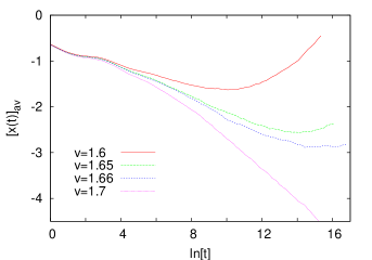
Figure 3: Left: Average position (horizontal coordinate) of a walker in time for different values of $v$ for the bimodal distribution in Eq.(9) with $c=0.4$ and $\lambda=0.1$ measured in Monte Carlo simulation. The direction of the motion is reversed at $v\approx 1.66$.

As seen in this figure, the direction of the walk has changed by varying $v$. For small lane change rate, $v<v_{c}\approx 1.66$ the walker goes ahead, whereas for large values of $v>v_{c}$, it moves backwards. At $v=v_{c}$ the average displacement tends to a constant in the limit $t\to\infty$. We have also studied the typical time-scale in the problem, $t_{L}\sim\Omega_{L}^{-1}$, by the renormalization method. According to phenomenological scaling at the recurrent point we have $\ln\Omega_{L}\sim L^{1/2}$ (see Eq.(1)) whereas, in the transient phase, the dependence is algebraic: $\Omega_{L}\sim L^{-1/\mu_{2}}$ (see Eq.(25)). In order to check both type of behavior, we have plotted $[\ln\Omega_{L}]_{\rm av}$ as a function of $L^{1/2}$ (Fig.4, left panel) and as a function of $\ln L$ (Fig.4, right panel).

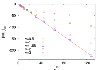
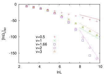
Figure 4: The average of the logarithm of the minimal exit rate, $[\ln\Omega_{L}]_{\rm av}$, plotted against $L^{1/2}$ (left panel) and against $\ln L$ (right panel) for the bimodal distribution used in Fig.3. At the recurrent point, $v=v_{c}$, the linear dependence in the plot in the left panel corresponds to Sinai-scaling in Eq.(1). In the transient phase, linear dependence is seen in the plot in the right panel, and the asymptotic values of the slopes identified with $1/\mu_{2}(v)$ depend on $v$ (see Eq.(25)).

The results in Fig.4 are in complete agreement with the scaling theory. In the transient phase, the diffusion exponent $\mu_{2}(v)$, which can be extracted from the asymptotic slopes of the curves in the right panel, are found to depend on $v$. We are going to study this issue in details for the symmetric disorder, where the condition of recurrence is exactly known.

For symmetric disorder we consider also two-lane systems and use the bimodal randomness in Eq.(6). In our first example we have $c=1/8$ and $\lambda^{2}=1/3$, which, according to Eq.(8), results in a diffusion exponent $\mu_{1}=1/3$ for $K=1$. By application of the renormalization group procedure we have calculated sample dependent minimal exit rates $\Omega_{L}$ and studied their distribution. For different lengths, $L$, the appropriate scaling combination is: $\Omega_{L}L^{1/\mu_{2}}$, see Eq.(25), and the distributions in terms of this reduced variable show a nice scaling collapse. This is illustrated in Fig.5 for the lane change rate, $v=0.1$, using a diffusion exponent $\mu_{2}=0.726$. The scaling curve is very well described by the Fréchet-distribution[28]:

$$P_{Fr}(u)=\mu_{2}u^{\mu_{2}-1}\exp(-u^{\mu_{2}})\;,$$ (26)

with $u=u_{0}\Omega_{L}L^{1/\mu_{2}}$. Here the non-universal constant, $u_{0}$, which depends on the amplitude of the tail of $P_{>}(\Omega)$ is the only free parameter.

The distribution of the low-energy excitations in strongly disordered systems has been studied previously in Ref.[29]. Using the strong disorder renormalization group method it has been argued that in several models the smallest excitations, the energy of which follow an asymptotic power-law behavior, can be considered asymptotically independent and therefore their distribution is in the Fréchet form. Our result in Fig.5 indicates that the disordered multi-channel problem satisfies this conjecture.

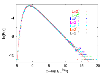
Figure 5: Distribution of the scaling variable $\Omega_{L}L^{1/\mu_{2}}$, calculated for $K=2$ with symmetric bimodal randomness ($c=1/8,~{}\lambda^{2}=1/3$ and $v=0.1$). The scaling collapse is obtained with a diffusion exponent $\mu_{2}=0.726$. The solid line is the Fréchet-distribution given in Eq.(26) with the parameter $u_{0}=0.392$.

We have repeated the previous renormalization group calculation for different values of $v$ and estimated the diffusion exponent by comparing the average value of $[\ln\Omega_{L}]_{\rm av}$ and that of $[\ln\Omega_{L/2}]_{\rm av}$. From this we have obtained effective exponents:

$$\mu_{2}^{\rm eff}(L)=\frac{[\ln\Omega_{L/2}]_{\rm av}-[\ln\Omega_{L}]_{\rm av}}{\ln 2}\;,$$ (27)

which are shown in the left panel of Fig.6 as a function of $\tau=L^{1/\mu_{2}}$. These exponents are compared with those calculated by the Monte Carlo simulations. In this case the average position of the walker, $[x(t)]_{\rm av}$, is calculated at time, $t$, and from the results at two different times, $t$ and $t\cdot\Delta$, we have obtained:

$$\mu_{2}^{\rm eff}(t)=\frac{\ln[x(t\cdot\Delta)]_{\rm av}-\ln[x(t)]_{\rm av}}{\ln\Delta}\;.$$ (28)

These are also shown in the left panel of Fig.6 as a function of $\tau=t$.

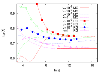
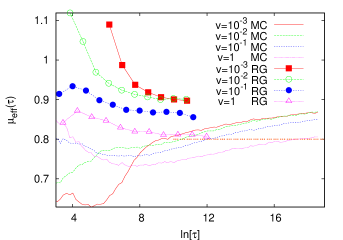
Figure 6: Effective diffusion exponent of the random walk in the two-channel problem for various values of the lane change rate, $v$, calculated either by the Monte Carlo simulations ($\tau=t$) or by the renormalization method ($\tau=L^{\mu_{2}}$). We used symmetric bimodal randomness. Left panel: $c=1/8,~{}\lambda^{2}=1/3$, so that $\mu_{1}=1/3$. Right panel: $c=1/3$, $\lambda^{2}=0.1768$, so that $\mu_{1}=0.4$.

As can be seen in this figure the calculated effective exponents have strong $\tau$ dependence for small systems (renormalization method) and for short times (simulation). However, the true exponents obtained by the two methods, which should be seen in the limit $\tau\to\infty$ seem to agree well. As expected, $\mu_{2}$ is a continuous function of the lane change rate and it is found to decrease monotonically with $v$. In the large $v$-limit it approaches the known exact limiting value: $\lim_{v\to\infty}\mu_{2}=2\mu_{1}$, see Eq.(16). Similar tendency is seen in the right panel of Fig.6 for different parameters of the distribution: $c=1/3$, $\lambda^{2}=0.1768$, so that $\mu_{1}=0.4$. In both distributions the diffusion exponent remains smaller than one, even for very small value of $v$, thus the system is always in the anomalous diffusion regime.

This type of behavior is going to change if we use such type of distributions, for which $\mu_{1}$ reaches or exceeds the value of $0.5$. In this case $2\mu_{1}\geq 1$, thus the transport in the two-lane system is ballistic. This type of behavior is illustrated in Fig.7 for $c=1/4$, $\lambda^{2}=1/9$, i.e. $\mu_{1}=0.5$ (left panel) and for $c=1/4$, $\lambda^{2}=1/5$, i.e. $\mu_{1}=0.683$ (right panel).

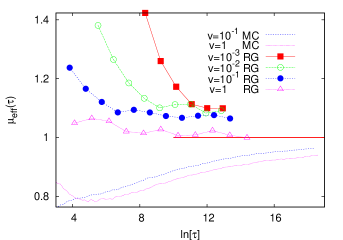
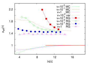
Figure 7: The same as in Fig.6 for ballistic transport. Here the $\mu_{\rm eff}$ calculated by the renormalization group method are the disorder induced diffusion exponents, which represent correction to scaling effects. Left panel: $c=1/4$, $\lambda^{2}=1/9$, so that $\mu_{1}=0.5$. Right panel: $c=1/4$, $\lambda^{2}=1/5$, thus $\mu_{1}=0.683$. Here we also present the exponent $3-\sigma$ (indicated by ”var”), in which $\sigma$ is the effective exponent of the second moment of the displacement measured in the simulations.

Indeed the effective exponents calculated by the Monte Carlo method approach one, which is a clear signal of the ballistic behavior. (We note that in the borderline case, $\mu_{K}=1$, there may be logarithmic corrections to the ballistic behavior just as for $K=1$ at $\mu_{1}=1$ [4])

In this case the exponent extracted from the finite size scaling of $\Omega_{L}$ is greater than $1$ and thus differs from the true diffusion exponent, which is equal to $1$. The exponent obtained by the renormalization in this phase appears in the corrections to scaling to the ballistic behavior. To be concrete, this exponent governs the scaling of the second moment of the displacement, $\Sigma_{L}$, which is expected to scale as $\Sigma_{L}\sim L^{\sigma}$, with $\sigma=3-\mu_{2}$. In the right panel of Fig.7 the renormalization estimates for $\mu_{2}$ are compared with the estimates for $3-\sigma$, which are obtained in Monte Carlo simulations and good agreement is found.

Finally, we mention that, for symmetric randomness, it is possible to drive the system from the sublinear transient phase to the ballistic phase by varying the lane change rate.

6 Discussion

In this paper we have studied the diffusion of a particle in a quasi-one-dimensional system which consists of $K$ disordered channels. We have investigated the transient phase by Monte Carlo simulations and by a variant of the strong disorder renormalization method. In this phase, the diffusion exponent is found to depend on $K$ and the lane change rate. For asymmetric disorder, the recurrent point is shifted compared to that of the one-lane model and the interaction between the lanes is able to cause a counter-intuitive reversal of the direction of motion when the lane change rate is varied. This phenomenon is analogous to the ratchet effect in a saw-tooth potential. For symmetric disorder the recurrent point stays invariant and the diffusion exponent in the transient phase is found to increase with $K$ and decrease with the lane change rate.

The numerical value of the diffusion exponent for $K>1$ and for intermediate lane change rates $0<v<\infty$ is non-trivial. It is easy to see, that a naive random trap description, when applied to the lanes separately, gives a wrong result. Indeed, identifying the trapping regions in each lane, then regarding them point-like traps which are concentrated on a single site would lead after simple argumentation on the probability of simultaneous occurrence of traps with a waiting time at least $t$ in all lanes to the diffusion exponent $\mu_{K}=K\mu_{1}$, independent of $v$ and the type of randomness. The problem with this argument is that, although, the finite extension of trapping regions does not play a role in one dimension, this circumstance cannot be disregarded in a coupled multi-channel system. After long times the particle may encounter long enough overlapping trapping regions in all lanes, where it cannot pass even in the most favourable lane without changing lanes. Such overlapping regions must be treated as a whole and they lead to a non-trivial dependence of the diffusion exponent on the distribution of transition rates.

The choice that the lane change rate is site-independent allows an alternative interpretation of the model. The particle can be thought to move in one-dimension but in a time-dependent potential, which fluctuates stochastically with rate $v$ between $K$ different random potentials each of which is determined by the jump rates in the $K$ lanes. A similar but spatially non-random problem, the first passage time of a particle over a homogeneous barrier the height of which fluctuates between two different values has been thoroughly studied [30, 31, 32] In case of very low flipping frequency the mean first passage time is dominated by first passage time over the higher barrier. For very high flipping frequency the particle feels an average potential and the first passage time is determined by the mean height of the potential. For intermediate frequencies the passing of the particle occurs primarily when the height of the barrier is small. Therefore, when varying the frequency, the mean first passage time exhibits a minimum. This phenomenon is called resonant activation. The optimal frequency is a known to decrease exponentially with the minimal height of the barrier [32].

Our result are qualitatively in agreement with the properties of resonant activation. For long times, the particle encounters higher and higher barriers, therefore the optimal lane change rate at which the release time is minimal becomes smaller and smaller as the particle proceeds. Consequently, for late times ($t\to\infty$), the diffusion exponent assumes its maximum in the limit $v\to 0$, in agreement with the numerical results. Note that these two limits can not be interchanged, therefore the (asymptotic) diffusion exponent of the model as a function of the lane change rate is non-analytical at $v=0$.

References

References

- [1] Alexander S, Bernasconi J, Schneider W R and Orbach R 1981 Rev. Mod. Phys. 53 175
- [2] Havlin S and Ben-Avraham D 1987 Adv. Phys. 36 695
- [3] Haus W and Kehr K W 1987 Phys. Rep. 150 263
- [4] Bouchaud J-P and Georges A 1990 Phys. Rep. 195 127
- [5] Solomon F 1975 Ann. Prob. 3 1
- [6] Kesten H, Kozlov M V and Spitzer F 1975 Compositio Math. 30 145
- [7] Sinai Ya G 1982 Theor. Prob. Appl. 27 247
- [8] Golosov A O 1984 Commun. Math. Phys. 92 491
- [9] Derrida B and Pomeau Y 1982 Phys. Rev. Lett. 48 627; Derrida B 1983 J. Stat. Phys. 31 433
- [10] Zeitouni O 2006 J. Phys. A: Math. Gen. 39 R433
- [11] Fisher D S, Le Doussal P and Monthus C 1998 Phys. Rev. Lett. 80 3539 Le Doussal P, Monthus C, and Fisher D S 1999 Phys. Rev. E 59 4795
- [12] Ma S-K, Dasgupta C and Hu C-K 1979 Phys. Rev. Lett. 43 1434
- [13] Fisher D S 1992 Phys. Rev. Lett. 69 534; 1995 Phys. Rev. B 51 6411
- [14] For a review, see: Iglói F and Monthus C 2005 Phys. Rep. 412 277
- [15] Chowdhury D, Santen L, and Schadschneider A, 2000 Phys. Rep. 329 199
- [16] J. Howard, Mechanics of Motor Proteins and the Cytoskeleton (Sinauer, Sunderland, 2001).
- [17] Key E S 1984 Ann. Prob. 12 529
- [18] Radons G 2004 Physica D 187 3 Fichtner A and Radons G 2005 New J. Phys. 7 30
- [19] Szász D and Tóth B 1984 J. Stat. Phys. 37 27 Alili S 1999 J. Stat. Phys. 94 469
- [20] Bolthausen E and Goldsheid I 2000 Commun. Math. Phys. 214 429
- [21] Bolthausen E and Goldsheid I 2008 Commun. Math. Phys. 278 253
- [22] Juhász R 2008 J. Phys. A: Math. Theor. 41 315001
- [23] J. Hooyberghs, F. Iglói and C. Vanderzande 2003 Phys. Rev. Lett. 90 100601; 2004 Phys. Rev. E 69 066140
- [24] Juhász R, Santen L and Iglói F 2005 Phys. Rev. Lett. 94, 010601; 2005 Phys. Rev. E 72 046129
- [25] Iglói F, Juhász R and Lajkó P 2001 Phys. Rev. Lett. 86 1343 Iglói F 2002 Phys. Rev. B 65 064416
- [26] Pigolotti S and Vulpiani A 2008 J. Chem. Phys. 128 154114
- [27] Monthus C and Garel T 2008 J. Phys. A: Math. Theor. 41 255002; 2008 J. Stat. Mech. P07002; 2008 J. Phys. A: Math. Theor. 41 375005
- [28] J. Galambos, 1978 The Asymptotic Theory of Extreme Order Statistics Wiley, New York
- [29] R. Juhász, Y.-C. Lin, and F. Iglói 2006 Phys. Rev. B 73 224206
- [30] Doering C R and Gadoua J C 1992 Phys. Rev. Lett. 69 2318
- [31] Bier A and Astumian R D 1993 Phys. Rev. Lett. 71 1649
- [32] Boguá M, Porrà J M, Masoliver J and Lindenberg K 1998 Phys. Rev. E 57 3990