Quantum Annealing with Jarzynski Equality

Abstract

We show a practical application of an well-known nonequilibrium relation, the Jarzynski equality, in quantum computation. Its implementation may open a way to solve combinatorial optimization problems, minimization of a real single-valued function, cost function, with many arguments. It has been disclosed that the ordinary quantum computational algorithm to solve a kind of hard optimization problems, has a bottleneck that its computational time is restricted to be extremely slow without relevant errors. However, by our novel strategy shown in the present study, we might overcome such a difficulty.

1 Introduction: Quantum Annealing

To reduce power loss in electric circuits, we have to minimize the circuit length. This kind of problems are formulated into a more generic task to minimize or maximize a real single-valued function of multivariables, cost function. This is called optimization problem [1]. To solve these problems is one of the most important tasks and has broad applications in science and engineering. Well-known examples with discrete variables are satisfiability problems, exact cover, maximum cut, Hamilton graph, and traveling salesman problem.

Most of the above exemplified cases are mapped into a generic problem to find the ground state for a kind of systems seen in statistical physics, spin glasses. Its Hamiltonian is denoted as $H_{0}$ in the present study. One of the generic algorithms to solve optimization problems in reasonable time by exploiting resources in physics is quantum annealing (QA) [2, 3, 4]. In QA, we introduce artificial degrees of freedom of quantum nature, noncommutative operators in order to induce quantum fluctuations.

$$H(t)=f(t)H_{0}+\left\{1-f(t)\right\}H_{1},$$ (1)

where $f(t)$ is assumed to be a monotonically increasing function satisfying $f(0)=0$ and $f(\tau)=1$. The annealing time is denoted by $\tau$. The transeverse-field operator for spin glasses is often used as a quantum fluctuation, $H_{1}=-\sum_{i}\sigma_{i}^{x}$. The quantum annealing starts from the ground state of $H_{1}$, a uniform linear combination of all spin configurations on the basis of $\sigma_{i}^{z}$. The quantum system is driven by gradually decreasing the quantum fluctuation according to $f(t)$. The adiabatic theorem guarantees that we can reach a nontrivial ground state of $H_{0}$ after sufficiently slow quantum sweep $\tau_{c}\sim 1/\Delta^{2}$, where $\Delta$ is the energy gap of the instantaneous quantum system (1) [5]. If we consider the cases in which the quantum system as in Eq. (1) has a minimum energy gap vanishing as $\Delta\sim\exp(-\alpha N)$ for increasing the system size $N$, QA does not work well in reasonable time [6, 7].

2 Jarzynski Equality

To overcome the above difficulty in hard optimization problems, we propose a novel method in conjunction with a theoretical piece from non-equilibrium statistical physics, the Jarzynski equality (JE), in the present study [8, 9]. The Jarzynski equality is written by an well-known expression as,

$$\left\langle\mathrm{e}^{-\beta W}\right\rangle=\frac{Z_{\tau}(\beta)}{Z_{0}(\beta)},$$ (2)

where the angular brackets denote the average over all realizations in a predetermined process starting from an initial equilibrium state and $W$ is the work done during the process. The partition functions for the initial and final Hamiltonians are written as $Z_{0}(\beta)$ and $Z_{\tau}(\beta)$ with inverse temperature $\beta$, respectively. We here shortly recall the formulation of JE for the classical system on a heat bath. Let us consider a thermal nonequilibrium process in a finite-time schedule $t_{0}=0\leq t\leq t_{n}=n\delta t$. Thermal fluctuations can be simulated by the master equation. The probability that the system is in a state $\sigma_{k}$ at time $t_{k}$ is denoted as $P(\sigma_{k};t_{k})$. The transition probability per unit time $\delta t$ is defined as $M(\sigma_{k+1}|\sigma_{k};t_{k})$. In the original formulation of JE, the work is defined as the energy difference merely attributed to the change of the Hamiltonian, but we can construct JE also in the case of changing the inverse temperature by defining the work as $-\beta W(t_{k})=-(\beta(t_{k+1})-\beta(t_{k}))H_{0}$ for the state $\sigma$. The left-hand side of JE can then be expressed as

$$\left\langle\mathrm{e}^{-\beta W}\right\rangle$$

$$=\sum_{\{\sigma_{k}\}}\prod_{k=0}^{n-1}\left\{\mathrm{e}^{-\beta W(t_{k})}\mathrm{e}^{\delta tM(\sigma_{k+1}|\sigma_{k};t_{k})}\right\}$$

$$\quad\times\tilde{P}(\sigma_{0};t_{0}),$$ (3)

where $\tilde{P}(\sigma_{0};t_{0})$ denotes the initial equilibrium distribution. Even if the transition term $\exp(\delta tM(\sigma_{k+1}|\sigma_{k};t_{k}))$ is removed in this equation, JE is trivially satisfied as one can simply confirm. A non-trivial feature of JE is in the insertion of the transition term. From Eq. (3), it is straightforward to prove JE by use of the detailed-balance condition. An observant reader may think the above formulation without any consideration of quantum nature is not available for the application to QA. Nevertheless we can apply the classical JE to QA by aid of the classical-quantum mapping [10].

3 Classical-quantum mapping

The classical-quantum mapping leads us to a special quantum system, in which the (instantaneous) equilibrium state of the above stochastic dynamics can be expressed as the ground state. A general form of such a special quantum Hamiltonian is given as $H_{q}(\sigma^{\prime}|\sigma;t)=I-\mathrm{e}^{\frac{\beta(t)}{2}H_{0}}M(\sigma^{\prime}|\sigma;t)\mathrm{e}^{-\frac{\beta(t)}{2}H_{0}}$. This Hamiltonian has the ground state as $|\Psi_{\mathrm{eq}}(t)\rangle=\sum_{\sigma}\mathrm{e}^{-\beta(t)H_{0}/2}|\sigma\rangle/\sqrt{Z(t)}$. The ground state energy is $0$, which can be explicitly shown by the detailed-balance condition. On the other hand, the excited states have positive-definite eigenvalues, which can be confirmed by the application of the Perron-Frobenius theorem.

In the above special quantum system, we can deal with a quasi-equilibrium stochastic process as an adiabatic quantum-mechanical dynamics in QA. Let us consider QA for the above special quantum system by setting the parameter corresponding to the temperature $T\to\infty$ ($\beta\to 0$). This condition gives the trivial ground state for $H_{1}$ in the preceding section with an uniform linear combination, similarly to the ordinary QA. If we change $T\to 0$ very slowly, one can obtain the ground state of $H_{q}$, which expresses the very low-temperature equilibrium state for $H_{0}$, the cost function of the optimization problem that we wish solve. We however consider to construct a protocol with the same spirit as JE by using the special quantum system to overcome the bottleneck of the ordinary QA as proposed in the following section.

4 Quantum Jarzynski annealing and its application

We prepare a trivial ground state with a uniform linear combination as the initial condition in the ordinary QA. This initial state corresponds to the high-temperature equilibrium state $|\Psi_{\mathrm{eq}}(t_{0})\rangle\propto\exp(-\beta(t_{0})H_{0}/2)|\sigma\rangle$ with $\beta(t_{0})\ll 1$. We introduce the exponentiated work operator $W_{\rm exp}(t_{k})=\exp(-(\beta(t_{k+1})-\beta(t_{k}))H_{0}/2)$. It looks like a non-unitary operator, but we can construct this operation by considering an extended quantum system [11, 12]. If we apply $W_{\rm exp}(t_{k})$ to the preceding quantum state $|\Psi_{\mathrm{eq}}(t_{k})\rangle$, it is changed into a state corresponding to the equilibrium distribution with the inverse temperature $\beta(t_{k+1})$. After then, the time-evolution operator $U(\sigma^{\prime}|\sigma;t_{k+1})=\exp(-\mathrm{i}\delta tH_{q}(\sigma^{\prime}|\sigma;t_{k+1})/\hbar)$ also does not alter this state, since it is the ground state of $H_{q}(\sigma^{\prime}|\sigma;t_{k+1})$. The resulting state after the repetition of the above procedure is

$$|\Psi(t_{n})\rangle\propto\prod_{k=0}^{n-1}\left\{W_{\rm exp}(t_{k})U_{k+1}(\sigma_{k+1}|\sigma_{k};t_{k})\right\}.$$

$$\quad\times|\Psi_{\mathrm{eq}}(t_{0})\rangle$$ (4)

This is essentially of the same form as Eq. (3). We measure the obtained state by the projection onto a specified state $\sigma^{\prime}$. The probability is then given by $|\langle\sigma^{\prime}|\Psi(t_{n})\rangle|^{2}$, which means that the ground state we wish to find is obtained with the probability proportional to $\exp(-\beta(t_{n})H_{0})$. If we continue the above procedure up to $\beta(t_{n})\gg 1$, we can efficiently obtain the ground state of $H_{0}$. This is called the quantum Jarzynski annealing (QJA) in the present study. Most of the readers, who are familiar with the ordinary computation, have considered that it may seem unnecessary to apply the time-evolution operator $U(\sigma_{k+1}|\sigma_{k};t_{k})$, which expresses change between states by quantum fluctuations, at the middle step between the operations of the exponentiated work operators $W_{\rm exp}(t_{k})$. The time-evolution operator does not mean an artificial control but describes the change by quantum nature during quantum computation, which is inherent property in quantum computation. However we here remember the nontrivial point of JE. Even if quantum nature affects the instantaneous quantum state, the property of JE guarantees that we keep the quantum state expressing the instantaneous equilibrium state. If one considers to simulate this procedure in “classical” computers, we have to need the repetition of the pre-determined process to deal with all fluctuations in the nonequilibrium-process average, since we assume an ensemble in equilibrium in the formulation of JE. However, when we implement QJA in “quantum” computation, we operate QJA to a single quantum system in principal since the classical ensemble is mapped to the quantum wave function. We do not need the repetition of the same procedure differently from the classical case [12].

Let us take a simple instance to search the minimum from a one-dimensional random potential, which is formulated as the Hamiltonian $H_{0}=-\sum_{i=1}^{N}V_{i}|i\rangle\langle i|$. Here $V_{i}$ denotes the potential energy at site $i$ and chosen randomly. We employ a linear schedule for tuning the parameter $\beta$ from $0$ to $100$. Figure 1 shows the plot for QJA (upper circles), which are fixed along the reference curves (solid curve) representing the instantaneous Gibbs-Boltzmann factor. In contrast, QA (lower triangles) can not sufficiently find the ground state since we consider a very short annealing is considered in this case.

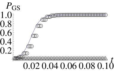
Figure 1: The performance of QA (triangles), and QJA (circles). The reference curve describes the instantaneous Gibbs-Boltzmann factor.

5 Summary

We consider an application of JE to quantum computation as QA to solve the optimization problems by using the classical-quantum mapping. As we expected, this protocol keeps the quantum system to express the equilibrium state for the instantaneous inverse temperature. The result by QJA shown here gives the ground state in a short annealing and implies that we may overcome the difficulties in hard optimization problems and solve them in a reasonable time. The present result is nothing but preliminary one. We should address the problem on practical efficiency for several interesting hard problems we wish to solve in the future study [13].

References

- [1] M. R. Garey and D. S. Johnson, Computers and Intractability: A Guide to the Theory of NP-Completeness Freeman, (San Francisco, 1979).
- [2] A. B. Finnila, M. A. Gomez, C. Sebenik, S. Stenson, and J. D. Doll, Chem. Phys. Lett. 219, 343 (1994).
- [3] T. Kadowaki and H. Nishimori, Phys. Rev. E 58, 5355 (1998).
- [4] S. Morita, and H. Nishimori, J. Math. Phys. 49, 125210 (2008).
- [5] S. Suzuki and M. Okada, J. Phys. Soc. Jpn. 74, 1649 (2005).
- [6] T. Jorg, F. Krzakala, J. Kurchan, A. C. Maggs, Phys. Rev. Lett. 101, 147204 (2008).
- [7] A. P. Young, S. Knysh, and V. N, Smelyanskiy, Phys. Rev. Lett. 104, 020502 (2010).
- [8] C. Jarzynski, Phys. Rev. Lett. 78, 2690 (1997).
- [9] C. Jarzynski, Phys. Rev. E 56, 5018 (1997).
- [10] R. D. Somma, C. D. Batista, and G. Ortiz, Phys. Rev. Lett. 99, 030603 (2007).
- [11] P. Wocjan, C. Chiang, D. Nagaj, and A. Abeyesinghe, Phys. Rev. A. 80, 022340 (2009).
- [12] M. Ohzeki, work in progress.
- [13] M. Ohzeki and S. Tanaka, work in progress.