City Size Distributions For India and China

Abstract

Abstract

This paper studies the size distributions of urban agglomerations for India and China. We have estimated the scaling exponent for the Zipf’s law with the Indian census data for the years of 1981-2001 and the Chinese census data for 1990 and 2000. Along with the biased linear fit estimate, the maximum likelihood estimate for the Pareto and Tsallis $q$-exponential distribution has been computed. For India, the scaling exponent is in the range of [1.88, 2.06] and for China, it is in the interval [1.82, 2.29]. The goodness-of-fit tests of the estimated distributions are performed using the Kolmogorov-Smirnov statistic.

pacs: 89.75.Da, 89.65.-s, 89.65.Gh

I Introduction

Nature, in spite of its complex character, often displays macroscopic regularity, which can be described broadly by simple laws at different scales. Examples include the size distribution of islands land and lunar craters lun , occurrence of forest fires forest and solar flares solar , websurfings web , wealth and income distribution in societies bkc , and also football goal distribution football . However, the size-distributions of populations in cities aces them all in arresting our longest attention chris .

It is conjectured that the city sizes obey a surprisingly simple law, known as Zipf’s law zipf (alternatively known as Pareto distribution or simply power law), which states that the population-wise rank, $R_{x}$, of a city with $x$ number of inhabitants is proportional to $x^{-\alpha}$, with $\alpha$ being close to one. This law has received empirical endorsement from different studies using data from USA, Switzerland switzerland , Brazil pro1 etc. However, fewer analysis have been conducted for urban agglomerations with comparatively lower populations. For example, a recent work jap shows that the size distribution of towns and villages are completely different from that of cities. Another interesting study stanley1 ; stanley2 looks at the spatial distribution of city population and observes deviation from the usual power law. Some other studies reveal that a deviation of the power law may be observed if all the urban agglomerations of an urbanized nation is considered japan ; mend . Some alternative statistical distributions mandl ; weibl ; mend are suggested to include the deviation from the power law. In general, the distribution of urban agglomerations in USA can be well-described by using a Tsallis $q$-exponential distribution mend , which is an extension of the standard Zipf-Mandelbrot law mandl proposed in the context of generalized statistical mechanics tsal .

The empirical phenomenon of the power law receives the theoretical support from some mathematical models mars ; simon ; dover . These theories model the evolution of the distribution of the city-size either as a time dependent process, or as a result of interactions among individuals. In both cases, reality is an approximation of the theoretical prediction of the limiting distribution and the empirically observed distribution converges to its limiting value depending on either the time-length of the process, or the total population of the considered society. This motivates us to analyze empirically the population distribution of cities for the two most populous countries of the world such as India and China, which are arguably the foremost ancient civilizations as well. These two countries are comparatively less urbanized and possess remarkably heterogeneous socio-economic structures. In any case, the data from India and China should be ideal to test the theoretical limiting predictions.

In this work, we carry out an empirical investigation with census data of India for the time period of 1981-2001 as well as with the Chinese census data for the years of 1990 and 2000. We estimate the scaling exponents for the Pareto distribution and also for a more generalized Tsallis $q$-exponential distribution. Also, goodness-of-fit tests for these hypothesized distribution have been performed. The methodology is described in Section II; whereas the data and the results are discussed in Section III. We conclude our study in the final section.

II Methodology

Let $p(\cdot)$ be a probability density function of the city-size distribution. The corresponding cumulative distribution function (CDF) and the complementary cumulative distribution function (CCDF) are given by $P(\cdot)$ and $P^{C}(\cdot)$, respectively. The CDF, $P(x)$ is the probability that a city has a population less than or equal to x and the CCDF, $P^{C}(x)$, is the probability that a city has a population greater than x. By definition,

$$P(x)=\int_{0}^{x}p(x^{\prime})dx^{\prime};~{}~{}~{}~{}P^{C}(x)=1-P(x)$$ (1)

In case of city-size distribution following the Zipf’s law,

$$p_{\alpha}(x)=Cx^{-\alpha}~{}~{}~{}\mbox{and}~{}~{}~{}\displaystyle P_{\alpha}^{C}(x)=\frac{C}{\alpha-1}x^{-(\alpha-1)}$$ (2)

where $\alpha$ and $C$ are constants. $\alpha$ is called the exponent of the power law. This family of power law distributions for $\alpha>1$ are known as the Pareto distribution. From equation (2), it is obvious that $p_{\alpha}(x)$ diverges to infinity for any value of $\alpha>1$ as $x\rightarrow 0$. Therefore, some minimum value, $x_{min}$, is usually considered for the support of the Pareto distribution. The corresponding probability density function, the CDF and the CCDF are given by:

$$p_{\alpha}(x)=\frac{(\alpha-1)\cdot x_{min}^{\alpha-1}}{x^{\alpha}};~{}~{}~{}~{}~{}~{}~{}P_{\alpha}(x)=1-\left(\frac{x_{min}}{x}\right)^{\alpha-1};~{}~{}~{}~{}~{}~{}~{}P_{\alpha}^{C}(x)=\left(\frac{x_{min}}{x}\right)^{\alpha-1}.$$ (3)

A more general distribution, namely the Tsallis $q$-exponential distribution, has been proposed in mend . The probability density function, the CDF and the CCDF of this distribution, as given in shalizi_MLE , are noted below:

$$p_{\theta,\sigma}(x)=\frac{\theta}{\sigma}\left(1+\frac{x}{\sigma}\right)^{-\theta-1};~{}~{}~{}~{}~{}P_{\theta,\sigma}(x)=1-\left(1+\frac{x}{\sigma}\right)^{-\theta};~{}~{}~{}~{}~{}P_{\theta,\sigma}^{C}(x)=\left(1+\frac{x}{\sigma}\right)^{-\theta}$$ (4)

From the equations (3) and (4), it is evident that the two distributions of Pareto and Tsallis q-Exponential are approximately identical for large values of $x$, when we set $\theta$ to $(\alpha-1)$ and $\sigma$ to $x_{min}$.

The slope of the plot, in which log of the rank of a city, $\log(R_{x})$, is plotted against the log of its population, $\log(x)$, has been used to estimate the exponent of the power law in almost all the previous studies. It has been shown shalizi_powerlaw that this produces a biased estimate of the power law exponent. Alternatively the Maximum Likelihood Estimator (MLE) produces the most efficient estimate. For a sample consisting cities with populations $x_{1}$, $x_{2}$, …, $x_{n}$, the log-likelihood of the sample is described by the following expression:

$$l(\underline{x};\nu)=\sum_{i=1}^{n}\log(p(x_{i};\nu))$$ (5)

where $p(x_{i};\nu)$ is the probability density function of the $i^{th}$ observation $x_{i}$ drawn from a certain distribution with parameter $\nu$. The function $l(\underline{x};\nu)$ is maximized with respect to the parameter $\nu$ to derive the maximum likelihood estimate $\widehat{\nu}$ of the parameter $\nu$. Mathematically,

$$\widehat{\nu}=\underset{\nu}{\arg\max}~{}~{}~{}l(\underline{x};\nu).$$ (6)

In particular, the MLE for the Pareto distribution with $x_{min}$ as the minimum value is given by:

$$\widehat{\alpha}_{MLE}=1+n\left[\sum_{i=1}^{n}\log\left(\frac{x_{i}}{x_{min}}\right)\right]^{-1}$$ (7)

The solution of the following system of simultaneous equations shalizi_MLE represents the MLE for the Tsallis $q$-exponential distribution with parameters $(\theta,\sigma)$ and $x_{min}$ as the minimum value:

$$\begin{array}[]{c}\widehat{\theta}_{MLE}=n\left[\sum_{i=1}^{n}\log\left(\frac{1+x_{i}/\widehat{\sigma}_{MLE}}{1+x_{min}/\widehat{\sigma}_{MLE}}\right)\right]^{-1}\\ \widehat{\sigma}_{MLE}=-\widehat{\theta}_{MLE}\frac{x_{min}}{1+x_{min}/\widehat{\sigma}}_{MLE}+\frac{\widehat{\theta}_{MLE}+1}{n}\sum_{i=1}^{n}\frac{x_{i}}{1+x_{i}/\widehat{\sigma}_{MLE}}\end{array}$$ (8)

The Fisher’s Information matrix crrao gives the asymptotic variance of the MLE. We can also compute the standard error in our estimate by the technique of Bootstrapping boot . In this method, we draw sub-samples from our original sample and compute the maximum likelihood estimates for those sub-samples. The standard error in the estimates obtained from different sub-samples is our estimate for the standard error of the MLE.

So far, we have treated $x_{min}$ as an exogenous parameter in estimating the scaling exponent. To derive shalizi_powerlaw an endogenous value for $x_{min}$, it is required to minimize the distance between the two CDFs, one obtained from the data and the other arising out of the best-fitted power law model, contingent on the value of $x_{min}$. In general, if we choose $\hat{x}_{min}$ higher than the true value of $x_{min}$, then the size of the data set is effectively reduced. Due to statistical fluctuations, a reduced data-set augments the error level for the empirical distribution, when compared with the fitted theoretical distribution. On the other hand, if $\hat{x}_{min}$ is smaller than the true value of $x_{min}$, the distribution will differ because of the fundamental difference between the data and the fitted model. Kolmogorov-Smirnov (KS) statistic KS is a standard measure to quantify this distance, $D$, between the two probability distributions with CDFs $F_{1}(\cdot)$ and $F_{2}(\cdot)$. Mathematically speaking,

$$D=\underset{x}{\sup}|F_{1}(x)-F_{2}(x)|$$ (9)

It may be worth noting that the CDF of the best-fitted power law depends on the choice of $x_{min}$ and $D$ is minimized with respect to this $x_{min}$. This leads to the optimal model, which is the closest one to the empirical distribution among the class of best fitted models. Simultaneously, we obtain $\hat{x}_{min}$, the optimal estimate for $x_{min}$.

Goodness-of-fit Tests

It might be interesting to test the null hypothesis crrao of empirical distribution following our estimated distribution (Pareto or Tsallis $q$-exponential). It should be mentioned here that even if we estimate the parameters of our distribution using the empirical observations, it is not anyway imperative for the observations to be actually from that particular distribution. We require a rigorous procedure shalizi_powerlaw to test the validity of our sample following the specified distribution.

After hypothesizing the empirical distribution from the optimal power law model, we simulate a similar sample from that particular distribution. The optimal power law model for the simulated sample is estimated by minimization of the relevant KS statistic over the values of $x_{min}$. Thereby, we obtain the optimal value for the KS statistic for this particular sample. If this value is greater than or equal to the corresponding value obtained from the actual data, it is an evidence in favour of the real data being from the best fitted power-law distribution. Otherwise, it is rather unlikely that the data is actually from the hypothesized power law distribution.

We generate a large number of samples with the same size as that of the data and calculate the fraction of samples, where the optimal KS statistic exceeds the one for the real data. We denote this fraction as the $p$-value of our test statistic. If this $p$-value is large, say close to one, then evidently the real data is from the best fitted power law distribution. On the other hand, if this $p$-value is close to zero, we fail to accept our hypothesis of data being drawn from a power law distribution. In terms of the level of the test, if the $p$-value is less than the specified level of the test, the null hypothesis of the data following a power law distribution is rejected.

We repeat this entire exercise for the null hypothesis of data following a Tsallis $q$-exponential distribution as well.

III Data Analysis and Results

Data Description

The Indian Census is conducted once in a decade. We have detailed data indiancensus for the year of 2001. According to the census conducted on the first day of March, 2001, the population of India stood at 1,027,015,247 persons. In that census data, there is a complete enumeration for the population of 4378 Indian urban agglomerations, 35 of which, have a population greater than a million. The data shows that only 27.86 percent of Indians live in these urban agglomerations; the rest of the Indians live in numerous rural agglomerations.

The People’s Republic of China conducted censuses in 1953, 1964, and 1982. In 1987 the government announced that the fourth national census would take place in 1990 and that there would be one every ten years thereafter. The 1982 census, which reported a total population of 1,008,180,738, is generally accepted as significantly more reliable, accurate, and thorough than the previous two. At the 2000 census, the total population stood at approximately 1.29533 billion, which is about 22% of total population in the world. 36% of the Chinese population used to reside in urban agglomerations in 2000. We use the data china_data from 1990 and 2000 census.

Study No.	Data-set	n	$x_{min}$	$x_{max}$	Mean	Median	Quartile 1	Quartile 3
I	India (2001)	3307	10.00	16434.39	84.30	23.42	15.39	48.23
II	India (2001)	174	203.38	16434.39	956.38	430.50	267.66	865.55
III	India (1991)	162	160.50	12596.24	759.45	365.31	219.75	654.49
IV	India (1981)	152	120.42	9194.02	576.86	277.22	171.68	519.37
V	China (2000)	1462	50.08	14230.99	298.27	136.63	80.86	265.42
VI	China (2000)	514	200.10	14230.99	658.95	358.81	254.67	578.36
VII	China (1990)	1345	25.02	7821.79	156.33	68.71	44.23	128.96
VIII	China (1990)	280	151.58	7871.79	503.05	274.58	189.83	456.18

Table 1: Data Description: Values of x (city-population) are reported in units of thousands. The left truncation of the data is determined through the value of $x_{min}$.
Source: indiancensus and china_data

In general, the theories for modeling the city-size distribution does not differentiate between an urban agglomeration and a rural one. However, the census data does not disclose the complete enumeration of the sizes for the rural agglomerations. Therefore, we analyze the size-distribution of the urban agglomerations alone. In the data, there are many towns with lesser number of inhabitants compared to that of many villages. If we consider the data for urban agglomerations in its entirety, this would lead to a biased data set for the population agglomerates as a whole and hence, to a biased set of estimates for the studied statistical models. This suggests us to consider the urban agglomerates over certain minimum value. We decide to set it at 10,000 for the Indian census data for the year of 2001. There is a trade-off involved in finding this minimum cut off for a town’s population size. The choice of a rather high value (say 20,000) causes us to loose a large fraction (nearly half) of our data set; whereas choice of a lower value would accentuate the problem of biased data-set. Most importantly, a small movement of the minimum value to either direction would not alter our estimates even quantitatively.

For the censuses of 1981 and 1991, we do not have the complete enumeration of the population figures in the Indian cities. However, we find the individual data for the population of Indian cities with a certain minimum number of inhabitants. For example, in 1991, we have individual data regarding 185 urban agglomeration with the total population of 125,457,068 persons; while the total urban population of India in 1991 was 217,611,012. Moreover, individual figures of all the cities above the population of 160,000 are included in these data. Therefore, we set the minimum value to 160,000 to left-censor our data-set. Further, to have a comparative study among the data from 1981, 1991 and 2001, we also work with all the Indian cities in 2001 with at least 200,000 dwellers.

We also use the individual data china_data on the population of urban agglomerations in China for the years of 1990 and 2000. We work with two different values for $x_{min}$ in both of these data-sets. The lower cut-offs (cases V and VII for the years 2000 and 1990) are chosen such as to include the data-set in its entirety baring a few outliers. The relatively higher cut-offs (as in cases VI and VIII for the years 2000 and 1990) are selected to compare the corresponding figures for the top ranking cities alone. It may be mentioned here that the distributions of Tsallis $q$-exponential and Pareto differ only at the lower level. We tabulate the descriptive statistics regarding all the data-sets in Table 1 for all the eight cases considered.

Results

We report the estimates corresponding to all the eight different cases studied in this paper in Table 2. We have elaborated the estimation procedure in Section II. The usual linear fit estimate using the Pareto Distribution is given by $\widehat{\alpha}_{lf}$; whereas the maximum likelihood estimate of the same is denoted as $\widehat{\alpha}_{MLE}$. It is emphasized here that the linear fit estimate, $\widehat{\alpha}_{lf}$, is not suitable for a proper estimation of the scaling parameter. As most of the prevalent literature has based their conclusion based on this measure, we compute it merely to measure the quantity and direction of the bias in this estimate. We find a considerable bias in the linear fit estimate compared to the corresponding one obtained using the technique of MLE. Also, the MLE of the parameters for the Tsallis $q$-exponential distribution are expressed as $\widehat{\theta}_{MLE}$ and $\widehat{\sigma}_{MLE}$ in Table 2. For each study, we plot the corresponding data-set and the fitted CCDFs. The graphical representation shows that in all the cases studied the estimated Pareto distribution and the fitted Tsallis $q$-exponential distribution are almost identical. Therefore, we restrict our attention to Pareto distribution alone for further investigation.

	Pareto		Tsallis		Minimized KS Distance Estimate with
Study No.	Distribution		Distribution		Pareto Dist.		Tsallis Dist.
	$\widehat{\alpha}_{LF}$	$\widehat{\alpha}_{MLE}$	$\widehat{\theta}_{MLE}$	$\widehat{\sigma}_{MLE}$	statistic	$p$-value	statistic	$p$-value
I	1.9923	1.8827	0.8827	0.0084	0.0348	0.000	0.0348	0.000
	(0.0010)	(0.0153)	(0.0002)	(0.0132)
II	1.9133	2.0320	1.0320	0.0530	0.0420	0.290	0.0420	0.286
	(0.0073)	(0.0782)	(0.0164)	(0.0709)
III	1.8946	2.0601	1.0601	0.0192	0.0648	0.005	0.0648	0.006
	(0.0083)	(0.0838)	(0.0025)	(0.0692)
IV	1.8893	1.9909	0.9909	0.0224	0.0557	0.052	0.0557	0.053
	(0.0085)	(0.0804)	(0.0027)	(0.0675)
V	1.8976	1.8480	0.8480	0.0120	0.0568	0.000	0.0568	0.000
	(0.0036)	(0.0222)	(0.0005)	(0.0167)
VI	1.7544	2.2975	1.2975	-0.1056	0.0217	0.531	0.0217	0.871
	(0.0018)	(0.0572)	(0.0424)	(0.0550)
VII	1.8967	1.8241	0.8241	0.0076	0.0682	0.000	0.0682	0.000
	(0.0031)	(0.0225)	(0.0001)	(0.0167)
VIII	1.7701	2.2308	1.2308	0.0666	0.0229	0.913	0.0229	0.913
	(0.0032)	(0.0736)	(0.0299)	(0.0675)

Table 2: Estimates from various data-sets considered: The standard errors are in parenthesis

In case of India, the estimated exponent ($\widehat{\alpha}_{MLE}$) is within the range of $[1.8827,2.0601]$ for different cases considered. The value is a good approximation of the theoretical predicted value of $2$ for $\alpha$. For China, $\widehat{\alpha}_{MLE}$ depends on the chosen value of $x_{min}$. It is in the range of $[1.8241,2.2975]$ contingent on the choice of $x_{min}$. For higher values of $x_{min}$, the estimate is bigger. It might be interesting to compare it with other studies. In case of cities of Brazil pro1 with $x_{min}$ as 30,000 the estimated value of $\alpha$ is found to be 2.41 for 1970 and 2.36 for 1980-2000. The corresponding linear fit estimate for 2400 U.S. cities switzerland is 2.1 for the year of 2000 and that for Switzerland stands at 2.0. The estimates using the data from Japan japan is rather interesting. It is shown that the Zipf’s law ($\alpha=2$) holds for the period of 1970-2000. Before and after this time period, $\alpha$ is significantly greater than 2. Using the KS statistic, we have computed the optimal estimate in the class of best fitted models and the endogenous value for $x_{min}$. In all the cases, it is almost same as the exogenously fixed value of $x_{min}$ in the data.

However, the data-set may contain a lot of non-sampling errors. The scatter plot reveals that the percentage of variation in our estimates is quite large, if we consider the slope of the fitted line neglecting a small number of observations. This is indicative of a poor quality of the data. So, we consider only two digits after the decimal place for all our estimates as significant. The interpretations for all the computed estimates in Table 2 should be modified accordingly.

A natural question may arise whether there is any other suggested distribution from the exponential family that explains the data better. There is an indication weibl that the Weibull distribution provides us a satisfactory adjustment for some ranges of the data. We carry out a likelihood maximization (LM) test crrao with our data-set, where the null hypothesis of data being from the Pareto distribution is tested against the alternative of various other statistical distributions, namely Weibull, Exponential, Exponential with a cutoff and log-normal. The $p$-value of the test statistic is always equal to one, which indicates that the null hypothesis is strongly accepted against the specified various alternatives. However, there is a word of caveat regarding this observation. The result does not imply that the assumption of the data following the Pareto distribution is justified. It is only a better description of the data over the other specified alternatives.

To test the validity of Pareto distribution, we compute the KS statistic as the distance between the empirical CDF and that of a fitted distribution as elaborated in Section II. The relevant $p$-values in Table 2 reveals that when we analyse the data comprising the sample of Indian cities with a higher $x_{min}$, the null hypothesis of Pareto distribution is accepted at the 5% critical level for all the years. But the null hypothesis can not be accepted if we consider the full sample for the year of 2001. In case of Chinese cities, the null hypothesis is again rejected with the full sample. However, it is well-accepted at any critical level, if the short sample with higher ranked cities is considered.

Finally, the graphical representation discloses that for both the countries of India and China, the comparatively higher ranked cities have disproportionately more dwellers compared to rather lower ranked ones. In general, the theories for size distribution implying Zipf’s law does not take into account any rural to urban migration, while modeling the distribution of urban agglomerations. However, it is an important phenomenon in the developing countries like India and China. In these countries, various Economic opportunities drive harris people from rural agglomerations to urban ones and also from smaller towns to larger cities. A theory, taking into account this factor, can explain the size distribution of the entire sample for the Indian (or Chinese) urban agglomerations.

IV Conclusion

In this work, we have shown that the city-size distribution for both the countries of India and China follow the Zipf’s law, if only we work with a more trimmed sample keeping the $x_{min}$ quite high. We have estimated the scaling exponent, by the linear fit method as well as by a more accurate technique of Maximum Likelihood Estimator, which is found to be nearly 2 as predicted. The maximum likelihood estimation with Tsallis $q$-exponential distribution is also performed, although the estimated CDF of this distribution is identical with its Pareto counterpart. The novelty of our work lies in the goodness-of-fit tests. The Kolmogorov-Smirnov statistic for the sample with the computed $p$-value implies that the full sample does not follow a Pareto or $q$-exponential Tsallis distribution too well. However, it gives a good approximation for a restricted sample with top ranking cities.

Acknowledgement: The authors thank Soumyasree Bandyapadhyay for compilation of data for this project.

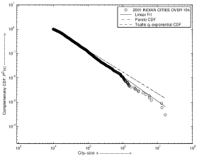
(a) Indian Cities with population over 10,000 in 2001

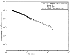
(b) Indian Cities with population over 200,000 in 2001

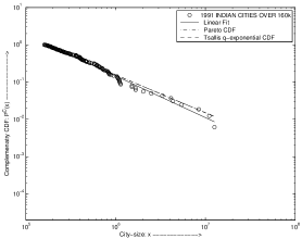
(c) Indian Cities with population over 160,000 in 1991

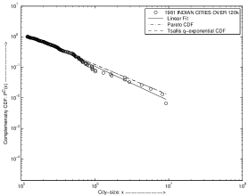
(d) Indian Cities with population over 120,000 in 1981

Figure 1: Indian Cities: 1981-2001

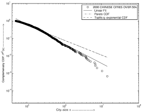
(a) Chinese Cities with population over 50,000 in 2000

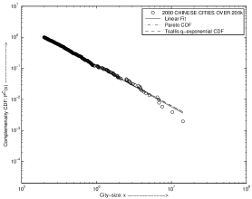
(b) Chinese Cities with population over 200,000 in 2000

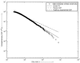
(c) Chinese Cities with population over 25,000 in 1990

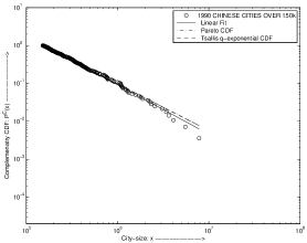
(d) Chinese Cities with population over 150,000 in 1990

Figure 2: Chinese Cities: 1990 and 2000

References

- (1) Y. Sasaki, N. Kobayashi, S. Ouchi1, and M. Matsushita, J. Phys. Soc. Jpn 75 (2006) 074804
- (2) R. B. Baldwin, Astron. Jour. 69(1964) 377
- (3) B.D. Malamud, G. Morein and D.L. Turcotte, Science 281 (1998) 1840
- (4) G. Boffetta,V. Carbone, P. Veltri, and A. Vulpiani, Phys. Rev. Lett. 83(1999) 4662
- (5) B.A.Huberman, P.L.T.Pirolli, J.E Pitkow and R.M.Lukose, Science 280(1998) 95
- (6) A. Chatterjee and B Chakrabarti, The European Physical Journal B 60 (2007) 135
- (7) L. C. Malacarne and R. S. Mendes , Physica A 286(2000) 391
- (8) W. Christaller, Central Places in Southern Germany (Prentice Hall Englewood Cliffs, NJ, 1933) (translated 1966)
- (9) G.K.Zipf, Human Behavior and the Principle of Least Effort (Addison-Wesley, Cambridge, MA, 1949)
- (10) D. Zanette and S.C. Manrubia, Phys. Rev. Lett.79 (1997) 523
- (11) N. J. Moura Jr. and M. B. Ribeiro, Physica A 367 (2006) 441
- (12) Y. Sasaki, H. Kuninaka, N. Kobayashi, and M. Matsushita, J. Phys. Soc. Jpn., Vol.76, No.7 (2007) 074801
- (13) H. D. Rozenfeld, D. Rybski, J. S. Andrade Jr., M. Batty, H. E. Stanley, and H. A. Makse, Laws of Population Growth Proc. Nat. Acad. Sci. 105 (2008) 18702
- (14) H. A. Makse, S. Havlin, and H. Eugene Stanley, Nature 377, (1995) 608
- (15) H. Kuninaka and M. Matsushita, J. Phys. Soc. Jpn., 77, No.11 (2008) 114801
- (16) L. C. Malacarne, R. S. Mendes, and E. K. Lenzi, Phys. Rev. E 65 (2002) 017106
- (17) B. B. Mandelbrot, The Fractal Geometry of Nature (Freeman, New York, 1977)
- (18) J. Laherrere and D. Sornette, Eur. Phys. Jour. B 2(1998) 525
- (19) C. Tsallis, J. Stat. Phys. 52 (1988) 479
- (20) M. Marsili and Y. C. Zhang, Phys. Rev. Lett. 80 (1998) 2741
- (21) Damian H. Zanette , Zipf’s law and city sizes: A short tutorial review on multiplicative processes in urban growth, (To appear in Advances in Complex Systems), arXiv:0704.3170v1
- (22) Y. Dover, Physica A 334(2004) 591
- (23) C. R. Shalizi, Maximum Likelihood Estimation for q-Exponential (Tsallis) Distribution, arxiv:math/0701854
- (24) A. Clauset, C. R. Shalizi, and M. J. Newman, Power-law distributions in empirical data, arxiv:0706.1062v1
- (25) C. R. Rao, Linear Statistical Inference and Its Applications, John Wiley and Sons, Inc (2002).
- (26) B. Efron and R. J. Tibsirani, An Introduction to the Bootstrap, Chapman and Hall, Boca Raton (1998).
- (27) I. M. Chakravarti, R. G. Laha, and J. Roy, Handbook of Methods of Applied Statistics, Volume I, John Wiley and Sons, (1967).
- (28) http://www.censusindia.gov.in
- (29) http://www.citypopulation.de/China.html
- (30) J. Harris and M. Todaro, American Economic Review, March 60(1) (1970) 126